Uncertainty Evaluation Based on Bayesian Transformations: Taking Facies Proportion as An Example

Abstract

Many input parameters in reservoir modeling cannot be uniquely determined due to the incompleteness of data and the heterogeneity of the reservoir. Sedimentary facies modeling is a crucial part of reservoir modeling. The facies proportion is an important parameter affecting the modeling results, because that proportion directly determines the net gross ratio, reserves and sandbody connectivity. An uncertainty evaluation method based on Bayesian transformation is proposed to reduce the uncertainty of the facies proportion. According to the existing data and geological knowledge, the most probable value of the facies ratio and the prior distribution of uncertainty are estimated. The prior distribution of the facies proportion is divided into several intervals, and the proportions contained in each interval are used in facies modeling. Then, spatial resampling is carried out for each realization to obtain the likelihood estimation of the facies proportion. Finally, the posterior distribution of the facies ratio is achieved based on Bayesian transformation. The case study shows that the uncertainty interval of sandstone proportion in the study area has been reduced from [0.31, 0.59] to [0.35, 0.55], with a range reduction of 29%, indicating that the updated posterior distribution reduces the uncertainty of reservoir lithofacies proportion, thereby reducing the uncertainty of modeling results.

1. Introduction

The heterogeneity of oil and gas reservoirs and the limited availability of information lead to great uncertainties in predicting reservoirs with these limited data. Especially for reservoirs in the early stages of exploration and development, where uncertainties in the geological understanding are even more pronounced due to the lack of wells. These uncertainties pose huge risks to the development of the reservoirs [1,2,3,4,5,6]. In order to reduce the risk of development decisions, the geological uncertainties need to be quantitatively evaluated and minimized. A growing number of domestic and foreign scholars have conducted research in this field [7,8,9,10,11,12,13,14,15]. Several reports at the AAPG annual meeting have discussed risk and uncertainty in oil exploration and development, pointing out that much of the risk arises from the uncertain understanding of subsurface reservoirs, and that uncertainty is usually underestimated [16]. Maschio et al. reported that production forecasting based on multiple realizations has become a consensus in the petroleum industry [13]. Caers discussed the role and significance of uncertainty modelling in the geosciences [17]. Li et al. detailed the basic concepts, principles, methods and application examples of reservoir uncertainty modeling, which discussed in detail the evaluation of uncertainty parameters, and methods to limit uncertainty [18].

The uncertainty parameters are closely related to the specific oilfield and to each development stage of the oilfield. The different range of uncertainty parameters largely determines the impact of that variable on the response index. Some variables have been studied relatively extensive by previous authors, such as the correlation of seismic attributes, the lower limit of porosity, and the oil‒water interface and so on. There are few studies on the parameters of sedimentary facies (lithofacies) ratio. The percentage of sedimentary facies directly decides the range of net gross ratio. The net gross ratio correlates with the volume and connectivity of sandbody, which is a critical parameter in reserve calculation and numerical simulation. Huo et al. selected six geological variables for reservoir modeling of an oil field in Bohai Bay [7], in which three level values for the percentage of distributary channel volume were given, but no details were given on how to set these three level values. Maschio et al. proposed to define the three level values for the lithofacies proportion using a discretization of the probability distribution function of the variables. The probability distribution is divided into three levels according to the occurrence probability, corresponding to level 0, level 1 and level 2, respectively [13]. Chong et al.’s strategy for the three values of the facies ratio parameter is to take the maximum, minimum and average value [19]. When modeling the sandbody, Xue et al. set six parameters, namely variance function, microfacies percentage, lower porosity limit, irreducible water saturation, volume coefficient and oil‒water interface. The three level values of microfacies percentage are given by using the data analysis function of the modeling software [20]. Some scholars have conducted special research on the uncertainty of the facies ratio parameter. André defined a statistical method to assess the uncertainty of the facies ratio, used the observed values to determine the analytical distribution of estimated values and proposed the theoretical framework of Dirichlet distribution [21]. Journel and Bitanov proposed a general uncertainty evaluation method to appraise the uncertainty of NTG (net to gross) by randomizing well locations [22]. In their workflow, the geological scenario, seismic data and initial drilling strategy are fixed. Conditional simulations are performed based on existing wells and seismic data, and then several different sets of virtual wells are sampled from the corresponding realizations. Each new set of data produces a new NTG estimate and the resampling results provide a measure of uncertainty. This idea of resampling from random realizations is known as spatial bootstrap. Unlike the classical bootstrap, it does not assume that the data along or between wells are independent [23,24,25,26]. Caumon et al. proposed a process framework to quantify the uncertainty of NTG. In contrast to Journel and Bitanov, who used a single prior NTG, they proposed to use a possible NTG prior distribution [27]. Mostafa adopts the method of unconditional sequential indicator simulation combined with spatial statistical resampling to quantify the uncertainty of a priori lithofacies proportion, and uses various realizations of a trend model to represent that uncertainty [28]. This specific approach is to take each realization as the input statistics of geostatistical modeling to obtain uncertainty models of posterior facies proportion uncertainty models.

In this article, a facies proportion uncertainty evaluation scheme based on Bayesian transformation is proposed. The uncertainty interval of the a priori facies ratio can be reduced by using the Bayesian method combined with facies data of the reservoir model. The basic idea of the method is to estimate the prior probability of variables (e.g., facies ratio) based on available information. The prior distribution of facies ratio is discretized into several intervals, and each interval is modeled. The likelihood estimation of facies proportion is obtained by spatial resampling for each realization. Finally, the posterior distribution of the facies ratio is obtained by Bayesian transformation.

2. Uncertainty Evaluation Workflow

2.1. Bayesian Theorem

The Bayesian theorem is a method to modify the subjective judgment of probability distribution (i.e., a priori probability) by using the observed phenomena in probability statistics. Unlike other methods, the Bayesian method is based on the subjective judgment of probability. It estimates a value from the existing experience and knowledge, and then continually revises that value according to the objective facts.

For two events A and B, the probability of A occurring under the condition of occurrence B is different from the probability of B occurring under the condition of occurrence of A. However, there is a deterministic relationship between the two, and the Bayesian rule is the expression of this relationship. The conditional and marginal probabilities formulas of the Bayesian rule for random events A and B are as follows:

$$P\left(A|B\right)=\frac{P\left(B|A\right)P\left(A\right)}{P\left(B\right)}$$

(1)

where $P(A|B)$ is the conditional probability of A after B is known to occur, called the posterior probability of A. $P(B|A)$ is the conditional probability of B after A is known to occur, called the posterior probability of B. $P\left(A\right)$ and $P\left(B\right)$ are respectively the prior or marginal probabilities of A and B.

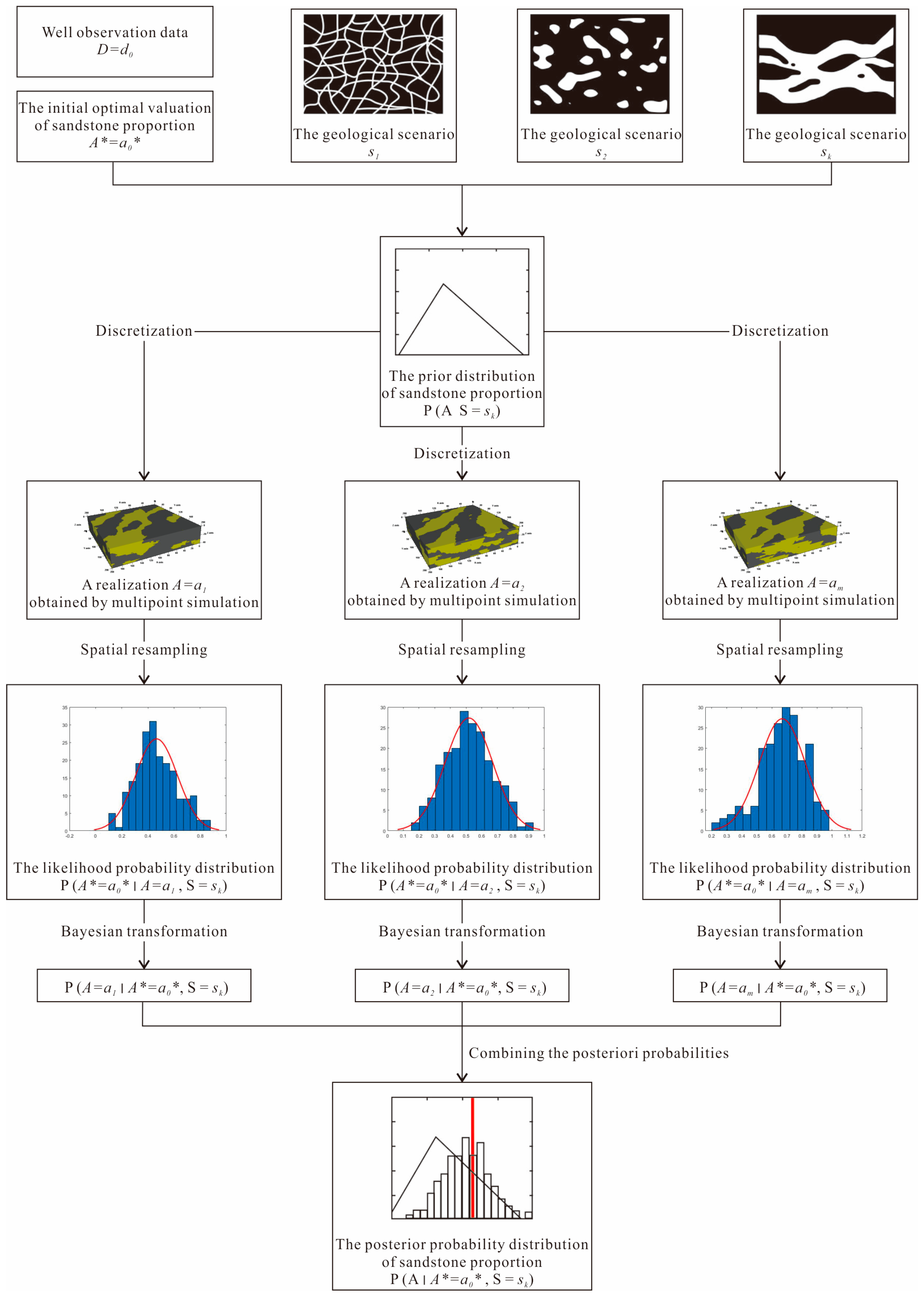
2.2. Uncertainty Evaluation Workflow Based on Bayesian Transformation

Taking facies proportion as an example, this manuscript describes the basic process of uncertainty evaluation. To simplify the problem, the lithofacies are divided into two categories, sandstone and mudstone. The sandstone proportions are considered as a random variable $D$, and the actual observed sandstone proportion is just one possible realisation of this random variable: $D=d_0$.

Figure 1 shows the detailed evaluation process. Several different geological scenarios, $S,$ are considered to obtain an uncertainty distribution of sandstone proportions. For a given realization, $s_{k,}$ of the geological scenario, a probability distribution, $P\left(A|S=s_k\right),$ of the sandstone proportions is determined by combining the existing cores, logs and seismic data in the work area. This distribution is used as the prior sandstone probability distribution in the Bayesian formula. The determination of the a priori distribution is subjective and usually relies on the experience of experts. Wells are mostly distributed in favorable areas, but a reliable initial best estimate should be given. Therefore, multiple virtual wells can be used to decluster the geological data of the reservoir model in the work area [29], so as to achieve the initial optimal sandstone proportional valuation, $A^{*}=a_0^{*}$. Subsequently, the prior distribution of sandstone ratio is updated according to $a_0^{*}$.

The distribution of a priori sandstone proportions is first uniformly dispersed into M classes from small to large: $a_1$, $a_2$, …, $a_m$. Random simulation is carried out for each type to obtain L sand‒mud lithofacies models. Then, the spatial statistical resampling method is used to resample the lithofacies model generated under each discrete class. Set a fixed number of virtual wells for random sampling N times (the well distribution is random). Each sampling will receive a sandstone proportion estimation, so the likelihood probability distribution of sandstone proportion under N sampling can be obtained. By this method, the likelihood probability, $P(A^{*}=a_0^{*}|A=a_m,S=s_k)$, of $a_0^{*}$ under a given geological background, $S=s_k$, and a given discrete level, $A=a_m,$ is determined.

Finally, Bayesian formula is used for the transformation to obtain the posterior probability of the sandstone proportion, $P(A=a_m|A^{*}=a_0^{*},S=s_k)$. The transformation formula is as follows:

$$P\left(A=a_m|A^{*}=a_0^{*},S=s_k\right)=\frac{P\left(A^{*}=a_0^{*}|A=a_m,S=s_k\right)\times P\left(A=a_m|S=s_k\right)}{P\left(A^{*}=a_0^{*}|S=s_k\right)}$$

(2)

where $P(A^{*}=a_0^{*}|S=s_k)$ is the marginal probability, which can be achieved by the total probability formula:

$$P\left(A^{*}=a_0^{*}|S=s_k\right)={\displaystyle \sum }_{m=1}^{M}P\left(A^{*}=a_0^{*}|A=a_m,S=s_k\right)\times P\left(A=a_m|S=S_k\right)$$

(3)

With the initial best estimate of the sandstone proportions for a given geological background, the process is repeated for the sandstone proportion value of each discrete class. The posterior probabilities at different discrete levels are acquired. The final posterior probability distribution of the true sandstone proportion is made by combination.

In practice, assigning a priori probabilities to different geological scenarios in the actual work area is a difficult task. One solution is to assume that each geological scenario is equally probable. Different experts give different estimates in combination with actual data and experience, and finally provide a reasonable estimation distribution, which can be triangular, Gaussian or uniform distribution.

3. Uncertainty Evaluation of the Facies Proportion in M Gas Field

M gas field is 439 km away from the southeast of Shanghai. It is located in the central inversion belt of Xihu Sag in the East China Sea continental shelf basin (Figure 2), and is a low-permeability gas reservoir. The reservoir was formed under the context of large-scale compression and contraction in Oligocene and belongs to reverse anticline structure. The strata in M gas field are deep buried. From bottom to top, the Eocene Pinghu Formation (E2p), Oligocene Huagang Formation (E3h), Miocene Longjing Formation (N1l), Yuquan Formation (N1y), Liulang Formation (N1ll) and Pliocene Santan Formation (N2s) are developed successively (Figure 3). The Huagang Formation is the main effective reservoir with little change in thickness. It can be divided into the upper section (H1–H5) and the lower section (H6–H7). The trap area of the target interval is 31.75~49.83 km².

Four wells have been drilled in the M gas field. The core and seismic data were used to explore the lithology, sedimentary structure, grain size and seismic profile characteristics. It is concluded that the Huagang Formation of the M gas field is a braided delta front deposit. The study focuses on the major underwater distributary channel, which is mainly formed by two sets of provenance from northeast and eastern. It shows the features of large sandbody thickness and multi-stage developed channels superposition. The H3b sublayer is the main gas-producing sand set, and the channel bar is the most favorable reservoir (Figure 4).

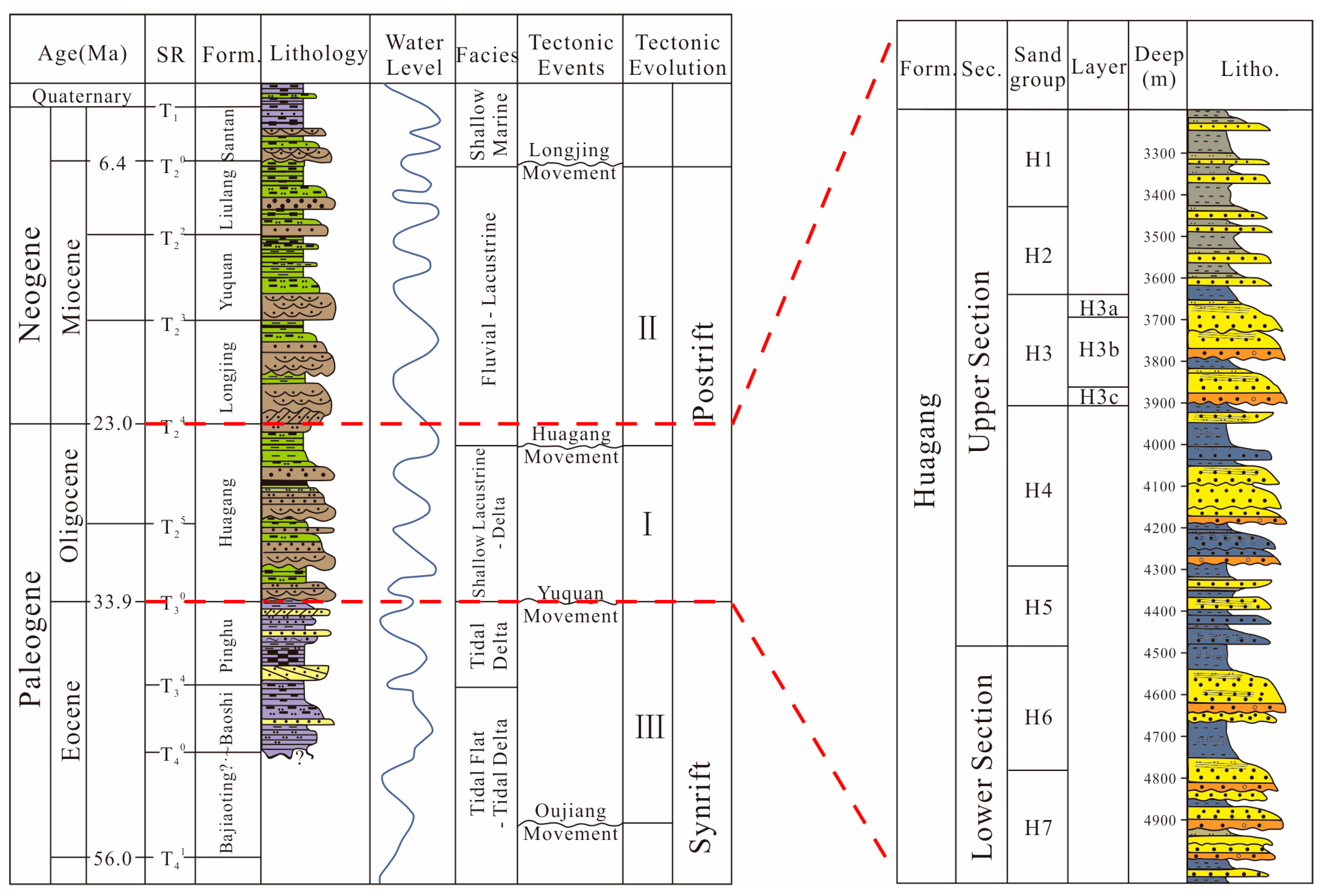
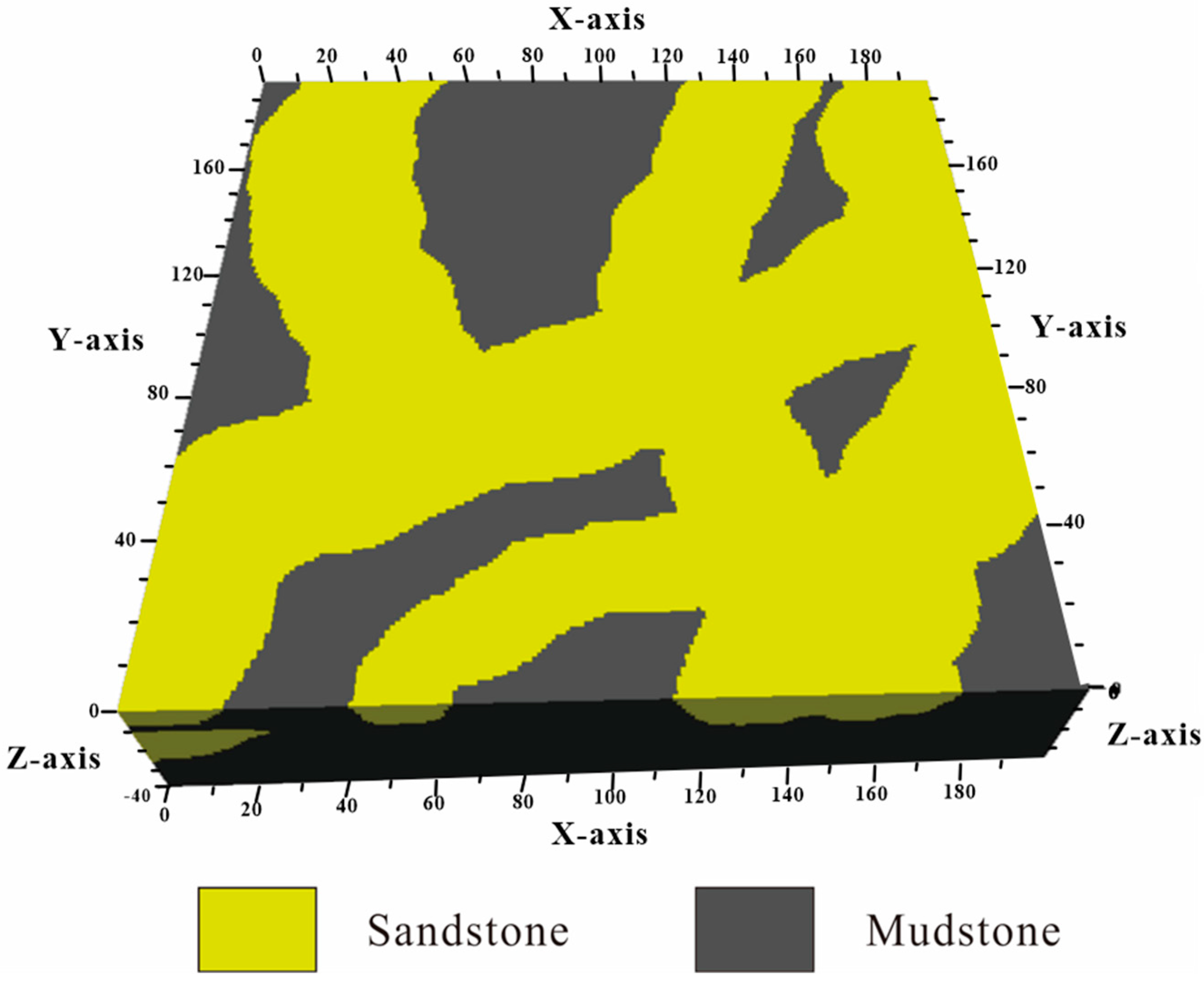
3.1. Establishment of Lithofacies Model

To simplify the problem, the distributary river channel and channel bar were combined into the sandstone facies. The distribution of sandbody thickness in the study area was counted, and information such as channel width was determined from seismic interpretation and prior knowledge. The 3D training image was created by using the object-based modeling approach (Figure 5). The river width was set at 1000 to 2000 m and the thickness was 10 to 20 m. The training image was divided into 100 × 100 × 40 grids, and the size of a single grid was 50 × 50 × 1 m. The initial sandstone proportion of the model was set to 0.45.

3.2. Determination of Prior Distribution of Sandstone Proportion

By averaging the sandstone proportion of four wells, the sandstone proportion obtained was 0.57, which is much higher than the most likely estimate given by experts of 0.45. Since these four wells were designed according to the favorable reservoir zone, the well statistics are higher than the proportion of sandstone in the whole gas reservoir.

In this case, due to the limited well data, a correction was needed for these data. For better estimation, the declustering algorithm was adopted. Thirty virtual wells were used to resample the above training image, and the declustering operation was performed on the resampled geological data to obtain the initial best estimate $a_0^{*}=0.44$. This value was more representative of all available data compared to the sandstone ratio value of 0.57, which was obtained from a single count of four wells.

Due to the high sandstone proportions of the well statistics, there was a possible bias. Therefore, an a priori sandstone proportion distribution with a mean value lower than the average sandstone proportion value of the wells was chosen. Here, a triangular distribution $P(A|S=S_k)$ with a mode of 0.45, a value of 0.2, and a maximum of 0.7 was used. This prior distribution is quite conservative with an uncertainty interval of $\left[\mathrm{P}10, \mathrm{P}90\right]=\left[0.31, 0.59\right]$. This interval included the average sandstone proportion of 0.57 from wells, the average sandstone proportion of 0.45 from the lithofacies model and also the corrected initial best valuation $a_0^{*}=0.44$. In general, the a priori sandstone ratio distribution provided should be obtained from the geological database of the simulated reservoir. This database depends on the different companies and contains the geology and exploration strategy for the work area.

The value $a_0^{*}=0.44,$ which was corrected by declustering, was used as the best estimate of the initial sandstone proportion, and then the prior distribution of sandstone proportion was updated for this given value.

3.3. Determination of Sandstone Proportion Likelihood Probability

The purpose of this workflow was to update the prior probability distribution through the likelihood probability distribution. Here, these likelihood probabilities $P(A^{*}=a_0^{*}|A=a_m,S=S_k)$ were calculated in the following ways.

(1)

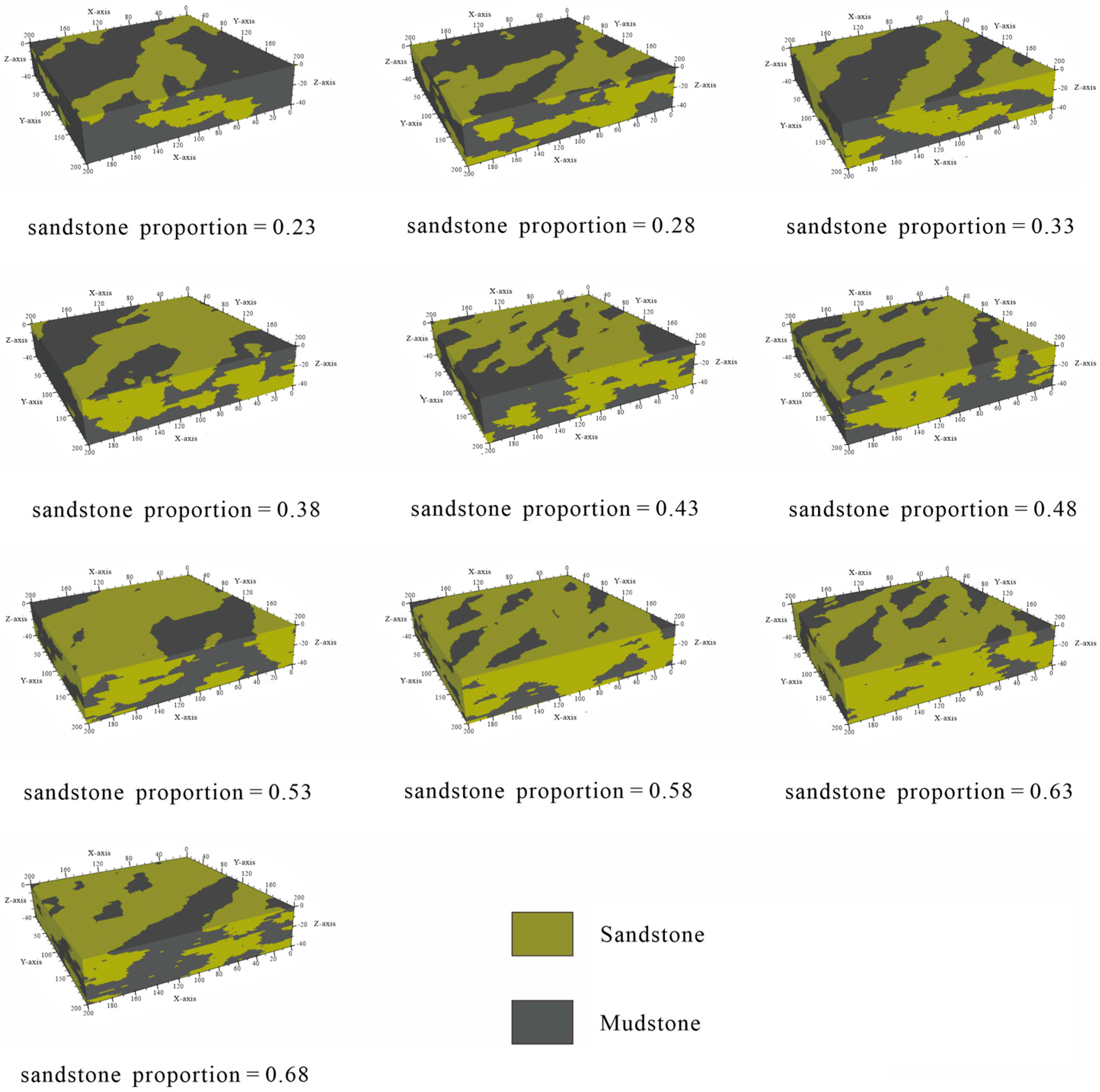
Ten target sandstone proportions were evenly selected between the minimum value of prior sandstone proportion distribution 0.2 and the maximum value 0.7. The proportional distribution of sandstone was divided into $m=10$ classes: $A=a_1$, $A=a_2$, …, $A=a_{10}$. Sandstone proportions were $a_1=\left[0.2, 0.25\right]$, $a_2=\left[0.25, 0.3\right]$, …, $a_{10}=\left[0.65, 0.7\right]$. Meanwhile, the median value of each interval was taken to calculate the prior probability of the corresponding discrete type (see

Table 1. The result of probability calculation ($m$ = 10).

Priori Probability	Likelihood Probability	Marginal Probability	Posterior Probability
0.0048	0.013	0.021652	0.002882
0.0128	0.06615		0.039106
0.0208	0.09525		0.091502
0.0288	0.12115		0.161145
0.0368	0.14		0.237946
0.0352	0.12945		0.210449
0.0272	0.12335		0.154957
0.0192	0.085		0.075374
0.0112	0.0385		0.019915
0.0032	0.0455		0.006725

).

(2)

The median value of sandstone proportion of each category was retained, and the SNESIM (single normal equation simulation) algorithm was used to simulate the multi point lithofacies. Ten lithofacies models were obtained (Figure 6).

(3)

The four wells in M gas field were used to spatially resample the random realization of these 10 multipoint simulations. A total of 200 samples were taken to obtain the likelihood probability distribution of the estimated sandstone proportion.

(4)

We substituted $a_0^{*}=0.44$ to calculate the likelihood probabilities at different discrete intervals. The results are shown in Table 1.

3.4. Determination of Sandstone Proportion Posterior Distribution

The calculated prior probabilities and likelihood probabilities were substituted into the Bayesian transformation formula (Equation (2)) and the total probability formula (Equation (3)) to calculate the posterior probabilities at the corresponding discrete level.

When this process was repeated for each discrete class, a posterior probability distribution of the true sandstone proportions for this geological scenario was given: $P(A=a_m|A^{*}=a_0^{*},S=S_k)$. The calculation results are shown in Table 1.

3.5. Results Analysis

The interval of the posterior distribution [P10, P90] was calculated to be [0.35, 0.55]. Compared to the previous distribution, the uncertainty interval of the updated posterior distribution was reduced by 29%, from the initial [P10, P90] probability interval [0.31, 0.59] to [0.35, 0.55]. In addition, the center values of the two distribution intervals were the same. This indicates that the prior distribution of sandstone ratio was quite in accordance with the observed quantitative data.

4. Analysis of Parameter Sensitivity

The experiment was further continued to identify several important factors that influenced the results. The analysis was carried out by (1) changing the discrete level of the prior distribution interval provided in the experiment, (2) changing the interval size of the prior distribution, and (3) changing the type of prior distribution.

4.1. Influence of the Number of Discrete Intervals

A triangular distribution with a plurality of 0.45, a minimum of 0.2 and a maximum of 0.7 was provided for the test. When achieving the likelihood probability distribution, 10 target sandstone proportions between 0.2 and 0.7 were selected. This means that the distribution was divided into $m=10$ classes. To test the effect of the discrete level on the experimental results, the distribution was further divided into 20 classes and $m=20$. The corresponding sandstone ratios were $a_1=\left[0.2, 0.225\right]$, $a_2=\left[0.225, 0.25\right]$, $a_3=\left[0.25, 0.275\right]$, …, $a_{20}=\left[0.675, 0.7\right]$. Repeating the previous Bayesian workflow, we retained the median of sandstone proportion in each class, and used the SNESIM algorithm to build the multipoint lithofacies model. Twenty models were produced, and then the likelihood probability distribution was obtained by spatial statistical resampling of each model. The prior and likelihood probabilities were received and brought into the Bayesian transformation equation to calculate the posterior probabilities. The results are shown in

Table 2. The results of probability calculations ($m$ = 20).

Priori Probability	Likelihood Probability	Marginal Probability	Posterior Probability
0.0016	0.0095	0.04318632	0.000351963
0.0064	0.0165		0.002445219
0.0096	0.032		0.007113364
0.0144	0.03425		0.011420283
0.0176	0.05195		0.021171519
0.0224	0.10425		0.054072679
0.0256	0.1073		0.063605327
0.0304	0.14175		0.099781598
0.0336	0.1315		0.102310176
0.0384	0.134		0.119148842
0.0384	0.1595		0.141822688
0.0336	0.1325		0.1030882
0.0304	0.13		0.09151046
0.0256	0.10305		0.061086011
0.0224	0.0825		0.042791328
0.0176	0.09		0.036678281
0.0144	0.0615		0.020506494
0.0096	0.06815		0.015149242
0.0064	0.034		0.005038633
0.0016	0.0245		0.000907695

.

Calculating $\mathrm{P}10$ and $\mathrm{P}90$ of the posterior probability at this time, we compared these values with those of $\mathrm{P}10$ and $\mathrm{P}90$ which were discretized into 10 classes. The data were plotted and compared visually, as shown in Figure 7.

According to Figure 7, it can be roughly inferred that the classification of discrete levels from 10 to 20 classes had little influence on the test results. Compared with the prior distribution, both posteriori distributions reduced the uncertainty. The primary $\left[\mathrm{P}10, \mathrm{P}90\right]$ of 20 classes was reduced to $\left[0.35,0.56\right]$, while this interval of 10 classes was $\left[0.35,0.55\right]$. The difference in $\mathrm{P}90$ values was very small, and the interval size was almost the same. Therefore, there was no need to increase the dispersion types in subsequent experiments. Setting the discrete level to 10 produced considerable experimental results. Increasing the dispersion level increased the workload, and the results showed no significant change.

4.2. Influence of Prior Distribution Interval

Considering that the provided prior distribution interval will affect the experimental results, the interval of prior distribution is further reduced in this section. Add two priori triangular distributions: triangular distribution 2 and triangular distribution 3. The distribution differs from the original triangular distribution1 in that it changes the size of the interval (

Table 3. The basic information of three prior distributions.

	Triangular Distribution 1	Triangular Distribution 2	Triangular Distribution 3	Gaussian Distribution	Uniform Distribution
Minimum	0.2	0.25	0.3	0.2	0.2
Maximum	0.7	0.65	0.6	0.7	0.7
P10	0.31	0.34	0.367	0.35	0.25
P50	0.45	0.45	0.45	0.45	0.45
P90	0.59	0.56	0.533	0.55	0.65

).

The Bayesian workflow was repeated with the provided triangular distribution 2 and 3. The discrete level was set to $m=10$ and the prior probabilities were calculated. The median sandstone proportions for each class were then retained and the lithofacies models was simulated using the multipoint simulation algorithm SNESIM. The models were resampled and the likelihood probabilities were counted, and finally the posterior probabilities were computed by combining the Bayesian formula. The experimental results are presented in

Table 4. The results of posterior probability calculation (Triangular Distribution 2).

Triangular Distribution(2)
Priori Probability	Likelihood Probability	Marginal Probability	Posterior Probability
0.005	0.0365	0.02692	0.006779
0.015	0.0555		0.030926
0.025	0.0819		0.07606
0.035	0.12815		0.166617
0.045	0.1281		0.214138
0.045	0.13405		0.224085
0.035	0.135		0.175523
0.025	0.075		0.069652
0.015	0.05		0.027861
0.005	0.045		0.008358

and

Table 5. The results of posterior probability calculation (Triangular Distribution 3).

Triangular Distribution(3)
Priori Probability	Likelihood Probability	Marginal Probability	Posterior Probability
0.0089	0.09705	0.044438	0.019437
0.0222	0.0925		0.046211
0.0356	0.1125		0.090127
0.0489	0.145		0.159561
0.0622	0.15		0.209958
0.0578	0.152		0.197707
0.0444	0.14015		0.140931
0.0311	0.127		0.088882
0.0178	0.0937		0.037533
0.0044	0.0975		0.009654

.

By calculation, $\mathrm{P}10=0.37$ and $\mathrm{P}90=0.53$ for triangular distribution 2, while the $\mathrm{P}10$ and $\mathrm{P}90$ values of triangular distribution 3 were 0.371 and 0.522 respectively. We compared the posterior interval results under three different distributions (Figure 8).

As can be seen from Figure 8 of the three distributions, the corresponding posterior interval $\left[\mathrm{P}10,\mathrm{P}90\right]$ will also be reduced if the prior interval size is reduced. These three triangular distributions reduced the uncertainty of sandstone facies proportion by applying Bayesian workflow. However, the uncertainty reduction degree of triangle distribution 3 was relatively low, and the interval of $\left[\mathrm{P}10,\mathrm{P}90\right]$ almost had no obvious reduction. It is considered that this was because the prior distribution range provided by distribution 3 itself was small and its uncertainty was relatively small, so the correction degree of Bayesian workflow was reduced accordingly.

4.3. Influence of the Priori Distribution Type

The previous section considered that the interval of the prior distribution provided affects the experimental results. The further testing found that different types of prior distributions also affected the results. Therefore, the type of prior distribution was changed and two additional prior distributions were added: Gaussian distribution and uniform distribution. The mathematical expectation of Gaussian distribution provided was $\mu =0.45$, and the standard deviation $\sigma =0.08$. The uniform distribution had a minimum value of $a=0.2$ and a maximum value of $b=0.7$. The intervals corresponding to their distributions are shown in Table 3.

Similarly, the Bayesian workflow was repeated for the Gaussian and uniform distributions. The discrete level was set to $m=10$ to calculate the prior probabilities. Lithofacies models were carried out using the multipoint simulation algorithm SNESIM, retaining the median sandstone proportions for each class. We resampled the models, and counted and calculated the likelihood probability. Finally, the posterior probabilities were obtained by combining the Bayesian formula and the results are shown in

Table 6. The results of posterior probability calculation (Gaussian Distribution).

Gaussian Distribution
Priori Probability	Likelihood Probability	Marginal Probability	Posterior Probability
0.00114	0.013	0.023858	0.000621
0.00522	0.06615		0.014473
0.01619	0.09525		0.064636
0.03401	0.12115		0.172699
0.04833	0.14		0.283599
0.04648	0.12945		0.25219
0.03025	0.12335		0.156395
0.01332	0.085		0.047455
0.00397	0.0385		0.006406
0.0008	0.0455		0.001526

and

Table 7. The results of posterior probability calculation (Uniform Distribution).

Uniform Distribution
Priori Probability	Likelihood Probability	Marginal Probability	Posterior Probability
0.02	0.013	0.017147	0.015163
0.02	0.06615		0.077156
0.02	0.09525		0.111098
0.02	0.12115		0.141308
0.02	0.14		0.163294
0.02	0.12945		0.150989
0.02	0.12335		0.143874
0.02	0.085		0.099143
0.02	0.0385		0.044906
0.02	0.0455		0.053071

.

The posterior probabilities obtained for each discrete level were combined to obtain the posterior probability distribution and the data were mapped for visual comparison (Figure 9).

From Figure 9, it can be seen that both the triangular and uniform distribution reduced the uncertainty of sandstone facies proportion after applying Bayesian workflow. However, the uncertainty interval $\left[\mathrm{P}10,\mathrm{P}90\right]$ of Gaussian distribution did not change obviously. It is thought that this was due to the fact that the Gaussian distribution itself provided a smaller range of intervals for the prior distribution and its uncertainty was relatively small, so the Bayesian workflow corrected it to a correspondingly less extent.

Providing a priori distributions is a subjective exercise, so it was important to provide a reasonable prior distribution in the experiment. This distribution could be either triangular distribution or uniform distribution. Although the two distributions were very different, they both had conservative intervals and roughly the same average sandstone proportions. In both cases, the uncertainty range shown by the posterior distribution was significantly reduced, and the average value of these posterior distributions was also close to the real sandstone proportion in the actual work area. It is also desirable that the distributions provided all have the same or close central values. The $\left[\mathrm{P}10,\mathrm{P}90\right]$ intervals given included the statistical well data of work area, the sandstone proportion from the training image and the corrected initial best estimate $a_0^{*}$. If the initial best estimate of sandstone ratio was significantly lower or higher than the estimate, the bias would not be corrected, but instead produce erroneous results.

5. Conclusions

(1)

For the uncertainty evaluation framework based on Bayesian transformation, it is shown that the initial probability interval $\left[\mathrm{P}10,\mathrm{P}90\right]$ narrows from $\left[0.31,0.59\right]$ to $\left[0.35,0.55\right]$, and the uncertainty range has been reduced by 29%. The updated posterior distribution reduces the uncertainty interval for the reservoir sandstone proportion. In addition, both distributions have the same central value, indicating that the prior distributions of sandstone proportion fairly agree with the quantitative observation data.

(2)

The parameter of discrete levels has little effect on the experimental results of the Bayesian evaluation framework. The initial $\left[\mathrm{P}10,\mathrm{P}90\right]$ shrinks to $\left[0.35,0.56\right]$ for a discrete 20 levels. At a dispersion of 10 levels, the initial $\left[\mathrm{P}10,\mathrm{P}90\right]$ narrows to $\left[0.35,0.55\right]$, with almost the same interval size. Therefore, there is no need to increase the discrete levels in the evaluation. A discrete level setting of 10 gives considerable experimental results. Increasing the discrete level instead increases the workload and there is no notable difference in the experimental results.

(3)

If the range of the prior interval is reduced, the corresponding posterior interval $\left[\mathrm{P}10,\mathrm{P}90\right]$ will also be reduced but the provided prior distribution intervals cannot be too small. When the prior distribution interval is small, the uncertainty is also relatively small, and the Bayesian workflow corrects for it to a lesser extent accordingly. It does not make sense to use a Bayesian framework in this case.

(4)

Different prior distribution types also have a great impact on the evaluation results. It is recommended that this distribution be a triangular or a uniform distribution. Moreover, the distributions provided should preferably have the same or close central values. The $\left[\mathrm{P}10,\mathrm{P}90\right]$ interval given shall include as far as possible the actual work area statistics of well data, the sandstone ratio values from the training image, and the corrected initial optimal estimate $a_0^{*}$. If the initial best estimate of sandstone proportion is much lower or higher than the estimate, it will produce wrong results without bias being corrected.

(5)

The workload of the proposed method is heavy. For a prior interval with large uncertainty, the posterior distribution whose interval has been narrowed can be given, so as to reduce the uncertainty. This technique avoids the errors caused by subjective judgment, thus minimizing the cognitive bias. It can improve the reliability of subsequent modeling and reduce the development risk.

References

1. Li, S.H.; Zhang, C.M.; Peng, Y.L.; Zhang, S.F.; Chen, X.M.; Yao, F.Y. Reservoir uncertainty evaluation. J. Xi’an Univ. Pet. Nat. Sci. Ed. 2004, 19, 16–25. [Google Scholar]
2. Wang, X.; Yu, S.; Li, S.; Zhang, N. Two parameter optimization methods of multi-point geostatistics. J. Pet. Sci. Eng. 2022, 208, 109724. [Google Scholar] [CrossRef]
3. Dai, W.Y.; Li, S.H.; Qiao, J.Y.; Liu, S.Y. Progress of reservoir uncertainty modeling. Lithol. Reserv. 2015, 27, 127–133. [Google Scholar]
4. Sun, L.C.; Gao, B.Y.; Li, J.G. A discussion on the method to study uncertainty of geologic modeling parameters. China Offshore Oil Gas 2009, 21, 35–38. [Google Scholar]
5. Oberkampf, L.W.; Sharon, M.; Brian, M. Error and uncertainty in modeling and simulation. Reliab. Eng. Syst. Saf. 2002, 75, 333–357. [Google Scholar] [CrossRef]
6. Wang, X.; Hou, J.; Li, S.; Dou, L.; Song, S.; Kang, Q.; Wang, D. Insight into the nanoscale pore structure of organic-rich shales in the Bakken Formation, USA. J. Pet. Sci. Eng. 2020, 191, 107182. [Google Scholar] [CrossRef]
7. Huo, C.L.; Liu, S.; Gu, L.; Guo, T.X.; Hong, Q.H. A quantitative method for assessing the uncertainty of the reservoir geological model. Pet. Explor. Dev. 2007, 34, 574–579. [Google Scholar]
8. Su, J.C.; Zhang, L.; Ma, X.F. Geological modeling in the initial stage of development of the fluvial reservoir. Lithol. Reserv. 2008, 20, 114–118. [Google Scholar]
9. Srivastava, R.M. The visualization of spatial uncertainty. AAPG Comput. Appl. Geol. 1994, 3, 339–345. [Google Scholar]
10. Kupfersberger, H.; Deutsch, C.V. Ranking stochastic realizations for improved aquifer response uncertainty assessment. J. Hydrol. 1999, 223, 54–65. [Google Scholar] [CrossRef]
11. Bárdossy, G.; Fodor, J. Evaluation of Uncertainties and Risks in Geology: New Mathematical Approaches for their Handling; Springer: Berlin/Heidelberg, Germany, 2013. [Google Scholar]
12. Wang, X.; Zhang, F.; Li, S.; Dou, L.; Liu, Y.; Ren, X.; Chen, D.; Zhao, W. Case Study in Gudong Oil Field, China. Geofluids 2021, 2021, 8821711. [Google Scholar]
13. Maschio, C.; Carvalho, C.P.V.; Schiozer, D.J. A new methodology to reduce uncertainties in reservoir simulation models using observed data and sampling techniques. J. Pet. Sci. Eng. 2010, 72, 110–119. [Google Scholar] [CrossRef]
14. Armstrong, M.; Ndiaye, A.; Razanatsimba, R.; Galli, A. Scenario reduction applied to geostatistical simulations. Math. Geosci. 2013, 45, 165–182. [Google Scholar] [CrossRef]
15. Wang, X.; Zhou, X.; Li, S.; Zhang, N.; Ji, L.; Lu, H. Mechanism Study of Hydrocarbon Differential Distribution Controlled by the Activity of Growing Faults in Faulted Basins: Case Study of Paleogene in the Wang Guantun Area, Bohai Bay Basin, China. Lithosphere 2022, 7115985. [Google Scholar] [CrossRef]
16. Smalley, P.C.; Begg, S.H.; Naylor, M.; Johnsen, S.; Godi, A. Handling risk and uncertainty in petroleum exploration and asset management: An overview. AAPG Bull. 2008, 92, 1251–1261. [Google Scholar] [CrossRef]
17. Caers, J. Modeling Uncertainty in the Earth Sciences; John Wiley & Sons: London, UK, 2011. [Google Scholar]
18. Li, S.H.; Zhang, C.M.; Duan, D.P.; Lu, Y. Principle and Application of Reservoir Uncertainty Modeling; Geological Publishing House: Beijing, China, 2020. [Google Scholar]
19. Chong, R.J.; Yu, X.H.; Li, T.T. Application of experimental design theory in stochastic reservoir model optimization. Oil Gas Geol. 2012, 33, 94–100. [Google Scholar]
20. Xue, Y.X.; Liao, X.W.; Huo, C.L.; Hu, Y.; Zhang, R.C. Uncertainty analysis of reserves of fluvial reservoir calculated by the geological model. Reserv. Eval. Dev. 2018, 8, 1–5. [Google Scholar]
21. Haas, A.; Formery, P. Uncertainties in Facies Proportion Estimation I. Theoretical Framework: The Dirichlet Distribution. Math. Geol. 2002, 34, 679–702. [Google Scholar] [CrossRef]
22. Journel, A.G.; Bitanov, A. Uncertainty in N/ G ratio in early reservoir development. J. Pet. Sci. Eng. 2004, 44, 115–130. [Google Scholar] [CrossRef]
23. Norris, R.J.; Massonnat, G.J.; Alabert, F.G. Early Quantification of Uncertainty in the Estimation of Oil-in-Place in a Turbidite Reservoir. In Proceedings of the SPE Technical Conference & Exhibition, Houston, TX, USA, 3–6 October 1993. [Google Scholar]
24. Journel, A.G. Resampling from stochastic simulations. Environ. Ecol. Stat. 1994, 1, 63–91. [Google Scholar] [CrossRef]
25. Efron, B.; Efron, P.A. Bootstrap Methods: Another Look at Jackknife; Breakthroughs in Statistics; Springer: New York, NY, USA, 1992. [Google Scholar]
26. Wang, X.; Liu, Y.; Hou, J.; Li, S.; Kang, Q.; Sun, S.; Ji, L.; Sun, J.; Ma, R. The relationship between synsedimentary fault activity and reservoir quality—A case study of the Ek1 formation in the Wang Guantun area, China. Interpretation 2020, 8, SM15–SM24. [Google Scholar] [CrossRef]
27. Caumon, G.; Strebelle, S.; Caers, J.K.; Journel, A.G. Assessment of Global Uncertainty for Early Appraisal of Hydrocarbon Fields. In Proceedings of the SPE Annual Technical Conference & Exhibition, Houston, TX, USA, 26–29 September 2004. [Google Scholar]
28. Hadavand, M.; Deutsch, C.V. Facies proportion uncertainty in presence of a trend. J. Pet. Sci. Eng. 2017, 153, 59–69. [Google Scholar] [CrossRef]
29. Li, S.H.; Liu, Y.G.; Wang, Y.Z. Application of Tyson polygon in declustering of geological data. Geophys. Geochem. Explor. 2011, 35, 562–564. [Google Scholar]
Figure 1. The evaluation process based on Bayesian method.
Energies 16 06951 g001
Figure 2. Structural distribution map of Xihu Sag. ((a). Location in the southeast of Shanghai, (b). Location of Xihu Sag, (c). Location of M gas field).
Energies 16 06951 g002
Figure 3. Schematic stratigraphic column of the Xihu Sag.
Energies 16 06951 g003
Figure 4. The distribution of the sandbody in small layers of H3b.
Energies 16 06951 g004
Figure 5. Training image.
Energies 16 06951 g005
Figure 6. The 10 multipoint random realizations.
Energies 16 06951 g006
Figure 7. The effect on sandstone proportions when discrete intervals have different numbers.
Energies 16 06951 g007
Figure 8. Influence of different prior distribution intervals on sandstone proportion.
Energies 16 06951 g008
Figure 9. Influence of different types of prior distribution on sandstone proportion.
Energies 16 06951 g009