Predictive Current Control of Sensorless Linear Permanent Magnet Synchronous Motor

Abstract

In the vector control system of a tubular oscillating permanent magnet synchronous linear motor, it is difficult to obtain accurate feedback information from the conventional mechanical sensors under bad and complex working conditions. This paper presents a new predictive current control designed to estimate the speed of the tubular oscillation permanent magnet synchronous linear motor. It implements two control techniques: The first technique is using the sliding-mode observer’s speed observer for speed estimation. The second is to design a deadbeat predictive current control to replace the PI regulator in the conventional current loop; it solves the difficulties of global optimization and PI parameter setting. The simulation and experimental results show that this method gives a good dynamic performance.

1. Introduction

The tubular oscillation motor has been widely used in industry and other fields. In the conventional vector control system, it is necessary to use position sensors such as an encoder to obtain the speed [1] and position [2] information when the motor rotates. However, there are many disadvantages when using speed and position sensors, which are particularly prominent under the condition of underground drilling. Firstly, the spatial position of the motor is too small to install the sensor. Even if the sensor is installed [3], the feedback line is easily damaged in high-frequency oscillation, which not only increases the cost, volume, and complexity [4] of the system but also reduces its reliability and the robustness of the system.

Some scholars have proposed a position- and speed-sensorless-control strategy to solve the problems mentioned above. Usually, after the estimation algorithm obtains the voltage and current that are easy to measure, the speed and position information of the motor can be estimated according to the mathematical model [5,6,7,8] of the motor to realize speed sensorless control. It can avoid the problems caused by using sensors and significantly reduce the overall size and cost.

The most commonly used sensorless control algorithms are mainly divided into two categories. One is for the control of the motor at zero and low-speed domains [9]. There are mainly the “INFORM” method [10], carrier frequency method [11], and high-frequency signal injection method [12,13]. These methods use the salient pole characteristics of the motor. Therefore, it is dependent on the actual parameters of the motor.

The other is to control the medium- and high-speed domains. The mature control algorithms in this speed domain mainly include the back EMF method [14,15], model reference adaptive method [16], sliding-mode observer method [17,18], and extended Kalman filter method [19]. Among these methods, the SMO has attracted much attention because of its good disturbance immunity [20] and less influence [21] by environmental uncertainties.

The sliding-mode observer method is mainly controlled by the sliding-mode variable structure to make the estimated value converge to the actual value. This is a nonlinear control strategy. Through the observation of the forward channel, the given current and feedback current can be obtained. Then, according to the difference between the given and feedback signals, the sliding-mode surface and the sliding-mode reaching-law function are designed. According to the obtained error value, the back EMF and speed of the motor are reconstructed.

The sliding-mode control algorithm has strong immunity and robustness. Although there is chattering and the chattering cannot be eliminated, it is less affected by model parameters due to the characteristic that the state point is not affected by external disturbances after reaching the sliding-mode surface [22] and can be widely used in various fields.

The SMO suffers from a chattering problem, which is caused by the high-frequency switching of the SMO. High-frequency switching is caused by the use of symbolic functions within the control structure. A low-pass filter (LPF) is added to the SMO to eliminate chattering. Applying the LPF causes a phase delay and gain attenuation. Scholars usually add additional compensation strategies to eliminate the impact of the LPF.

On the other hand, because of the existence of sliding-mode chattering, the influence of current harmonics will be amplified, resulting in large fluctuations in speed. In order to solve this problem, controllers based on proportional resonance controllers, repetitive controllers, and iterative learning controllers have been proposed [23,24,25]. However, the parameters of the controllers often need to be adjusted with the harmonic frequency. Due to the fact that the PI controller can control the DC qualities and avoid the influence change, it is widely used in these problems [26,27]. However, the PI controller’s parameters tuning is as difficult as using multiple PI controllers.

Aiming at the above problems, this paper presents a new predictive current-control designed to estimate the speed of the motor. It has two parts: the sliding-mode observer and the current controller of deadbeat current predictive. The sliding-mode observer aims to solve the disturbance in an uncertain environment and achieve a better speed estimation. The current controller is designed to simplify the structure of the current loop, avoid the difficulties of global optimization and PI parameter setting, and suppress the impact of LPF. The main contributions of this study are as follows:

(1)

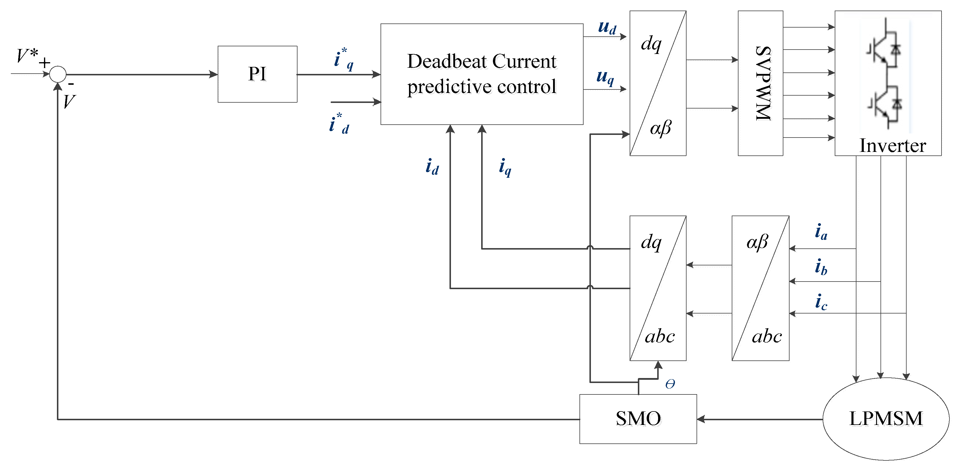
The SMO is used to observe the LPMSM velocity value, which reduces the impact of environmental uncertainty disturbance.

(2)

The deadbeat current predictive controller is designed to replace the PI controller. The influence of sliding-mode-observer chatter is reduced. It solves the problem that the PI controller’s parameters’ tuning is difficult.

(3)

The new deadbeat predictive current control has a better performance compared with the PI control.

The rest of the paper is organized as follows. Section 2 introduces the design of a sliding-mode speed observer based on LPMSM and proves the stability of the SMO. Section 3 explains how to design a deadbeat current control controller. Section 4 and Section 5 verify the superiority of the method through a simulation and experiment. Finally, Section 6 offers some concluding remarks.

2. Design of Sliding-Mode Speed Observer Based on LPMSM

For the cylindrical slotless, coreless LPMSM motor studied in this paper, the sliding-mode control designs the observer based on the error between the given current and feedback current, reconstructs the back EMF of the motor from the error, and estimates the motor position and speed information. Since the model equation in the two-phase rotating d–q coordinate system does not directly display the position information, the sliding-mode observer is constructed based on the mathematical model. In the two-phase stationary coordinate system, the voltage equation of LPMSM can be described as follows:

$$\{\begin{array}{c}{u}_{\alpha }=R_s{i}_{\alpha }+L_{s}p{i}_{\alpha }-\frac{\pi }{\tau }{n}_p{\phi }_f{v}_{m}sin\theta \\ u_{\beta }=R_s{i}_{\beta }+L_{s}p{i}_{\beta }+\frac{\pi }{\tau }{n}_p{\phi }_f{v}_{m}cos\theta \end{array}$$

(1)

where $u_{\alpha }$ and $u_{\beta }$ are the axis stator voltages, $i_{\alpha }$ and $i_{\beta }$ are the stator currents, ${\phi }_f$ is the rotor permanent magnet flux, $R_s$ is the stator resistance, $L_s$ is the axis inductance, $n_p$ is the pole pitch, $v_m$ is the speed of LPMSM, $p$ is a different operator, and $\tau$ is polar distance.

Then Equation (1) is transformed into Equation (2):

$$\{\begin{array}{c}{u}_{\alpha }=R_s{i}_{\alpha }+L_{s}p{i}_{\alpha }-e_{\alpha }\\ u_{\beta }=R_s{i}_{\beta }+L_{s}p{i}_{\beta }+e_{\beta }\end{array}$$

(2)

where $e_{\alpha }$ and $e_{\beta }$ are the components of back EMF on axes $\alpha$ and $\beta$, respectively.

$$\{\begin{array}{c}{e}_{\alpha }=\frac{\pi }{\tau }{n}_p{\phi }_f{v}_{m}sin\theta \\ e_{\beta }=\frac{\pi }{\tau }{n}_p{\phi }_f{v}_{m}cos\theta \end{array}$$

(3)

It can be seen from Equation (3) that the back EMF of the motor contains the speed information of the motor, so the back EMF signal can be extracted, and the position information of the motor can be solved. Now Equation (3) is changed to the form of a current state equation:

$$\{\begin{array}{c}p{i}_{\alpha }=\frac{1}{L_s}\left(u_{\alpha }-e_{\alpha }-R_s{i}_{\alpha }\right)\\ p{i}_{\beta }=\frac{1}{L_s}\left(u_{\beta }-e_{\beta }-R_s{i}_{\beta }\right)\end{array}$$

(4)

where $p$ is the differential operator.

Take the control function U(x) =$Ksign\left(x\right)$. The gain of the sliding-mode observer is $K$, and the sliding surface function is $s\left(x\right)$.

$$s\left(x\right)=\{\begin{array}{c}{\widehat{i}}_{\alpha }-i_{\alpha }\\ {\widehat{i}}_{\beta }-i_{\beta }\end{array}$$

(5)

The equation of the LPMSM current sliding-mode observer in a two-phase static coordinate system is as follows:

$$\{\begin{array}{c}p{\widehat{i}}_{\alpha }=\frac{1}{L_s}\left(u_{\alpha }-R_s{\widehat{i}}_{\alpha }-Ksign\left({\widehat{i}}_{\alpha }-i_{\alpha }\right)\right)\\ p{\widehat{i}}_{\beta }=\frac{1}{L_s}\left(u_{\beta }-R_s{\widehat{i}}_{\beta }-Ksign\left({\widehat{i}}_{\beta }-i_{\beta }\right)\right)\end{array}$$

(6)

where ${\widehat{i}}_{\alpha }$ and ${\widehat{i}}_{\beta }$ are the estimated values of the motor’s stator current components. The $sign$ symbolic function is selected as the control function in the sliding-mode observer. It can be described as follows (7):

$$sign\left(x\right)=\{\begin{array}{cc}1& x>0\\ 0& x=0\\ -1& x<0\end{array}$$

(7)

The current state equation can be obtained by subtracting Equation (4) from Equation (6), as shown in Equation (8):

$$\{\begin{array}{c}p\widetilde{i_{\alpha }}=\frac{1}{L_s}\left(e_{\alpha }-R_s\widetilde{i_{\alpha }}-Ksign\left(\widetilde{i_{\alpha }}\right)\right)\\ p\widetilde{i_{\beta }}=\frac{1}{L_s}\left(e_{\beta }-R_s\widetilde{i_{\beta }}-Ksign\left(\widetilde{i_{\beta }}\right)\right)\end{array}$$

(8)

where $\widetilde{i_{\alpha }}$ and $\widetilde{i_{\beta }}$ are the errors between the actual values of current components and the observed values.

$$\{\begin{array}{c}\widetilde{i_{\alpha }}={\widehat{i}}_{\alpha }-i_{\alpha }\\ \widetilde{i_{\beta }}={\widehat{i}}_{\beta }-i_{\beta }\end{array}$$

(9)

According to Equations (5) and (9) and $S=\dot{S}=0$, Equation (10) can be obtained:

$$\{\begin{array}{c}{S}_{\alpha }={\widehat{i}}_{\alpha }-i_{\alpha }=0\\ S_{\beta }={\widehat{i}}_{\beta }-i_{\beta }=0\\ e_{\alpha }=Ksign\left({\widehat{i}}_{\alpha }-i_{\alpha }\right)\\ e_{\beta }=Ksign\left({\widehat{i}}_{\beta }-i_{\beta }\right)\end{array}$$

(10)

As the actual control quantity is a discontinuous high-frequency switching signal, in order to extract the estimation value of continuous extended back EMF, it is usually necessary to add a low-pass filter, which is shown in Equation (11):

$$\{\begin{array}{c}{\widehat{e}}_{\alpha }=\frac{{\omega }_c}{s+{\omega }_c}{e}_{\alpha }\\ {\widehat{e}}_{\beta }=\frac{{\omega }_c}{s+{\omega }_c}{e}_{\beta }\end{array}$$

(11)

where ${\omega }_c$ is the cutoff frequency of the first-order low-pass filter, and ${\widehat{e}}_{\alpha }$ and ${\widehat{e}}_{\beta }$ are the estimated values of back EMF components on axes α and β, respectively.

According to the relationship between motor position and back EMF, the motor speed information can be calculated as shown in Equation (12):

$$v_m=\frac{p\ast \left(-\arctan \left(\frac{{\widehat{e}}_{\alpha }}{{\widehat{e}}_{\beta }}\right)\right)\ast \tau }{\pi n_p}$$

(12)

Then the estimated speed is as follows:

$${\widehat{v}}_m=\frac{\frac{\sqrt{{\widehat{e}}_{\alpha }{}^2+{\widehat{e}}_{\beta }{}^2}}{{\phi }_f}\tau }{\pi n_p}$$

(13)

The designed sliding-mode observer is analyzed by the Lyapunov stability theory, and the Lyapunov function is constructed as follows:

$$\dot{V}=S^T\dot{S}$$

(14)

Expand and verify Equation (14):

$$\begin{array}{cc}\hfill \dot{V}=\frac{1}{L_s}\{-R_s{\widetilde{i_{\alpha }}}^2& -R_s{\widetilde{i_{\beta }}}^2+\widetilde{i_{\alpha }}\left[e_{\alpha }-Ksign\left(i_{\alpha }\right)\right] +\widetilde{i_{\beta }}\left[e_{\beta }-Ksign\left(i_{\beta }\right)\right]\}\hfill \\ \hfill & =-\frac{R_s}{L_s}\left({\widetilde{i_{\alpha }}}^2+{\widetilde{i_{\beta }}}^2\right)+\frac{1}{L_s}\{\widetilde{i_{\alpha }}\left[e_{\alpha }-Ksign\left(i_{\alpha }\right)\right]\hfill \\ \hfill & +\widetilde{i_{\beta }}\left[e_{\beta }-Ksign\left(i_{\beta }\right)\right]\}\hfill \end{array}$$

(15)

According to Equation (15), $-\frac{R_s}{L_s}\left({\widetilde{i_{\alpha }}}^2+{\widetilde{i_{\beta }}}^2\right)<0$ is always established. Therefore, if $\dot{V}<0$, the condition of Equation (16) needs to be satisfied:

$$\frac{1}{L_s}\left\{\widetilde{i_{\alpha }}\left[e_{\alpha }-Ksgn\left(i_{\alpha }\right)\right]+\widetilde{i_{\beta }}\left[e_{\beta }-Ksgn\left(i_{\beta }\right)\right]\right\}<0$$

(16)

That is, it needs to satisfy $K>\max \left(\left|e_{\alpha }\right|,\left|e_{\beta }\right|\right)$.

3. Deadbeat Predictive Current Control

The current state equation of the LPMSM control system is shown in Equation (17):

$$\{\begin{array}{c}p{i}_{\mathrm{d}}=\frac{u_{\mathrm{d}}}{L_{\mathrm{d}}}-i_{\mathrm{d}}\frac{R_{\mathrm{s}}}{L_{\mathrm{d}}}+\frac{\pi }{\tau }{v}_m\frac{L_{\mathrm{q}}}{L_{\mathrm{d}}}{i}_{\mathrm{q}} \\ p{i}_{\mathrm{q}}=\frac{u_{\mathrm{q}}}{L_{\mathrm{q}}}-i_{\mathrm{q}}\frac{R_{\mathrm{s}}}{L_{\mathrm{q}}}-\frac{\pi }{\tau }{v}_m\frac{L_{\mathrm{d}}}{L_{\mathrm{q}}}{i}_{\mathrm{d}}-{\phi }_{\mathrm{f}}\frac{\pi }{\tau }{v}_m\end{array}$$

(17)

The sampling time, $T_s$, is extremely small, and it can be neglected. Therefore, Equation (17) can be discretized by using the first-order Taylor formula. It can be approximated to have the following equation:

$$\{\begin{array}{c}p{i}_{\mathrm{d}}=\frac{i_{\mathrm{d}}\left(k+1\right)-i_{\mathrm{d}}\left(k\right)}{T_{\mathrm{s}}}\\ p{i}_q=\frac{i_{\mathrm{q}}\left(k+1\right)-i_{\mathrm{q}}\left(k\right)}{T_{\mathrm{s}}}\end{array}$$

(18)

For the tubular oscillatory LPMSM, $L_d=L_q=L$. By applying Equation (18) to Equation (17) and rearranging the equations, the discretized current prediction model of LPMSM is obtained.

$$\{\begin{array}{c}{i}_d\left(k+1\right)=\frac{T_s}{L}\left[u_d\left(k\right)-R_s{i}_d\left(k\right)+L\frac{\pi }{\tau }{v}_m\left(k\right)i_q\left(k\right)\right]+i_d\left(k\right) \hfill \\ i_q\left(k+1\right)=\frac{T_s}{L}\left[u_q\left(k\right)-R_s{i}_q\left(k\right)-L\frac{\pi }{\tau }{v}_m\left(k\right)i_d\left(k\right)-L\frac{\pi }{\tau }{\phi }_f{v}_m\left(k\right)\right]+i_q\left(k\right)\hfill \end{array}$$

(19)

Using the reference current $s i_d^{\ast }\left(k\right)$ and $i_q^{\ast }\left(k\right)$ as the input currents $i_d\left(k+1\right)$ and $i_q\left(k+1\right)$ at instant $\left(k+1\right)$, the current $i_d\left(k\right)$ and $i_q\left(k\right)$ can be obtained by the three-phase current through mathematical frame axes transformation. The voltage mathematical model of LPMSM can be obtained through transformation, as shown below:

$$\{\begin{array}{c}{u}_d\left(k\right)=L\left(\frac{i_d{}^{\ast }\left(k\right)-i_d\left(k\right)}{T_s}\right)+R_s{i}_d\left(k\right)-L\frac{\pi }{\tau }{v}_m\left(k\right)i_q\left(k\right) \\ u_q\left(k\right)=\left(\frac{i_q{}^{\ast }\left(k\right)-i_q\left(k\right)}{T_s}\right)+R_s{i}_q\left(k\right)+L\frac{\pi }{\tau }{v}_m\left(k\right)i_d\left(k\right)+\frac{\pi }{\tau }{\phi }_f{v}_m\left(k\right)\end{array}$$

(20)

4. Simulation Analysis

In order to verify the control effects, the simulation model of two control strategies is built, sequentially. On the one hand, the speed-sensorless VC of the tubular oscillatory LPMSM is compared with the VC. On the other hand, the speed-sensorless DBPC of the tubular oscillatory LPMSM is compared with the speed-sensorless VC. It verifies the feasibility and superiority of the speed-sensorless DBPC.

4.1. Simulation Results of SMO

The control strategy using the SMO sensorless control was simulated. In this work, $i_d$ is controlled to zero. The parameters used to simulate the model are reported in

Table 1. Simulation parameters.

Symbol	Value	Unit
$L$	0.0085	[H]
$R_s$	2.875	[$\mathsf{\Omega }$]
${\psi }_f$	0.175	[Wb]
$n_p$	4	-
$\tau$	3	cm
$M$	4.3	[kg]
$B_v$	1.3	[N·s/m]

.

Set the command speed of LPMSM to 3 m/s, start without load, add 5 N·m load after 0.3 s, and reduce the speed to 1.5 m/s after 0.4 s. The simulation response results are shown in Figure 1, Figure 2, Figure 3 and Figure 4. The VCS means the vector control of sensorless. DBPCS means the deadbeat current control of sensorless.

It can be seen from Figure 1 that the overall speed following the effect is good and the dynamic response is fast. However, the speed overshoot is large during deceleration. This is because the proportional coefficient is large during the PI parameter adjustment, which accelerates the response speed and increases the overshoot at the same time.

Figure 2 shows the speed error between the observed and actual values. When the speed reaches a steady state, the speed error is almost 0 m/s. Sliding-mode observers can achieve a better speed estimation. However, the speed error increases when changing speed and loading. The reason may be that, when the speed changes, the PI controller controls the object to restore the steady state. Because the parameters cannot be adjusted adaptively, the proportional integral coefficient is large at this time, resulting in a large overshoot.

Figure 3 shows that the currents of the d-axis and q-axis fluctuate. Although the overall follow-up effect is good and the fluctuation is little, due to the inevitable chattering phenomenon of the sliding-mode observer itself, the d-axis current fluctuates around zero, and the q-axis current has a similar phenomenon

According to Figure 4, the comparison between the observed value and the actual value of the angle, when the error between them is close to zero, the estimated angle will be inaccurate due to the measured back EMF and the functional relationship of the sliding surface. This time is infinitesimal. It can be seen from the figure that, when the time is greater than zero, the angle tracking is more accurate. Although there is an error value, the error value is small, with only about 0.002.

Through the simulation model, the feasibility of the designed sliding-mode observer replacing the speed and position sensors in the traditional LPMSM control system was verified. The control effect shows that the designed observer has good accuracy, good follow-up, strong dynamic response performance, and strong anti-interference ability. However, because the current loop controller uses the traditional PI controller, the controller cannot adaptively adjust the parameters with the change of the controlled object, and it is not suitable for the condition of multi-working conditions and variable load, thus resulting in the poor dynamic response performance of the system under the condition of variable load and variable speed. On the other hand, the VCS control current fluctuates to some extent, due to the existence of sliding-mode chattering, under the same PI parameters, when the motor is running at variable speed or load; and the overshoot, when the speed reaches the steady state, increases significantly, indicating that the PI controller is greatly affected by chattering and is difficult to overcome. Therefore, in order to reduce the influence of sliding-mode chattering under the traditional PI control, a deadbeat current predictive controller is proposed to replace the traditional PI current control.

4.2. Simulation Results of SMO and DBPC

To realize the current predictive control of the sensorless LPMSM, the DBPC is presented to replace the traditional PI current loop in the SMO speed-sensorless control. Figure 5 shows the control structure of the method.

The method is simulated and analyzed; i_d is controlled to zero, and the parameters adopted in the simulation model are shown in Table 1. Figure 6, Figure 7 and Figure 8 show the simulation results.

In the control process, the speed is first set to 3 m/s, and then to 0.4 m/s at 0.4 s. In addition, a load of 5 N·m is applied at 0.3 s.

Figure 6 shows the simulation results of the estimated speed. The control strategy has a large overshoot when it is started at no-load, and the disturbance and dynamic-response characteristics before speed change are similar to those of the vector-sliding mode’s sensorless control. However, the overshoot of the control method is less than that of the sensorless control strategy when the speed drops at 0.4 s.

It can be seen from Figure 7 that, under the same load, the q-axis current after coordinate transformation under the control of DBPCS is smaller than that under the control of VCS, but the current fluctuation is large at the same time.

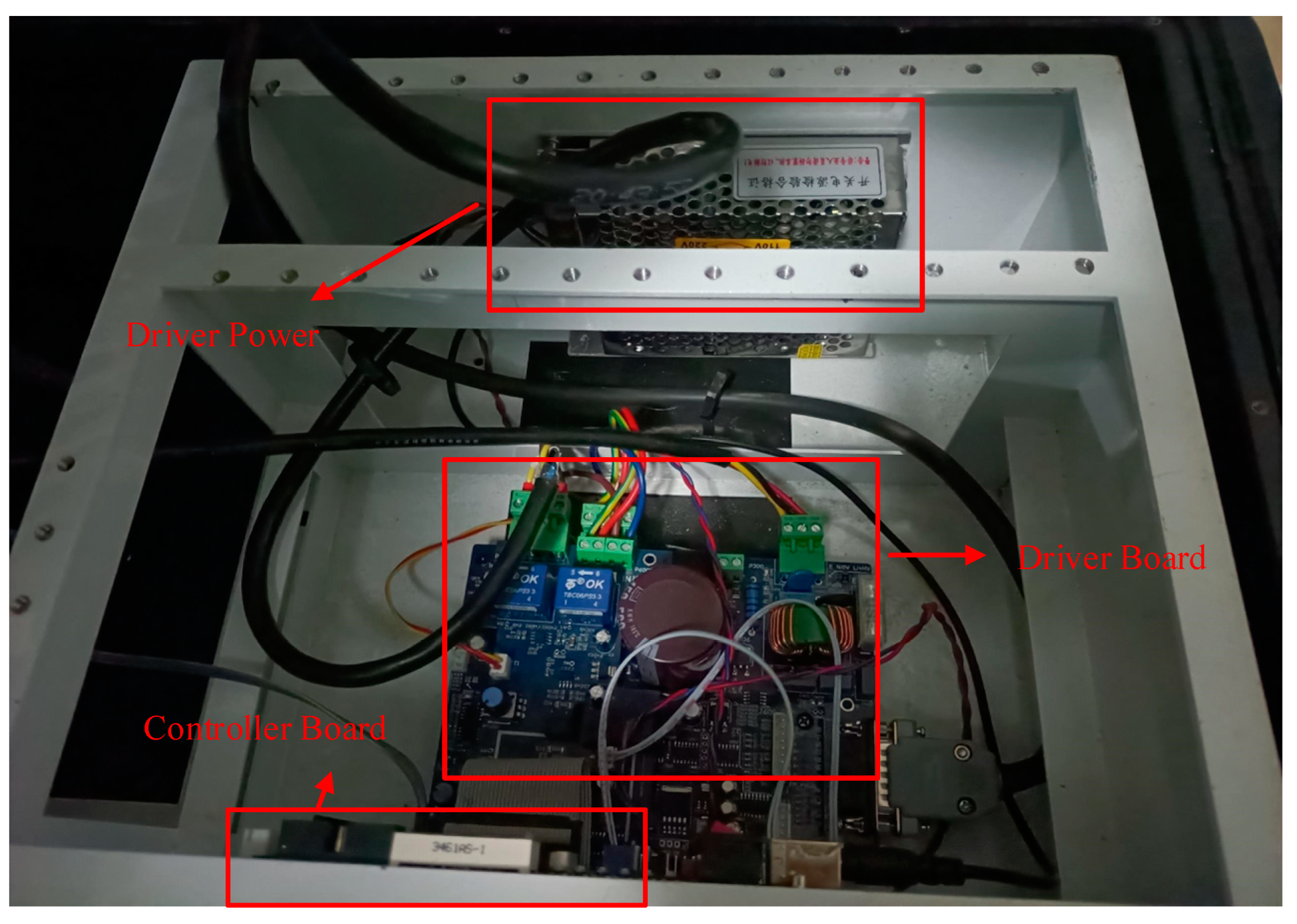
5. Analysis of Experimental Results

Figure 8 and Figure 9 show the LPMSM experimental platform, which includes the personal computer, laboratory box, LPMSM, etc. The main parameters of the motor are consistent with the simulation parameters. The acquisition frequency set in this control system is 1 kHz.

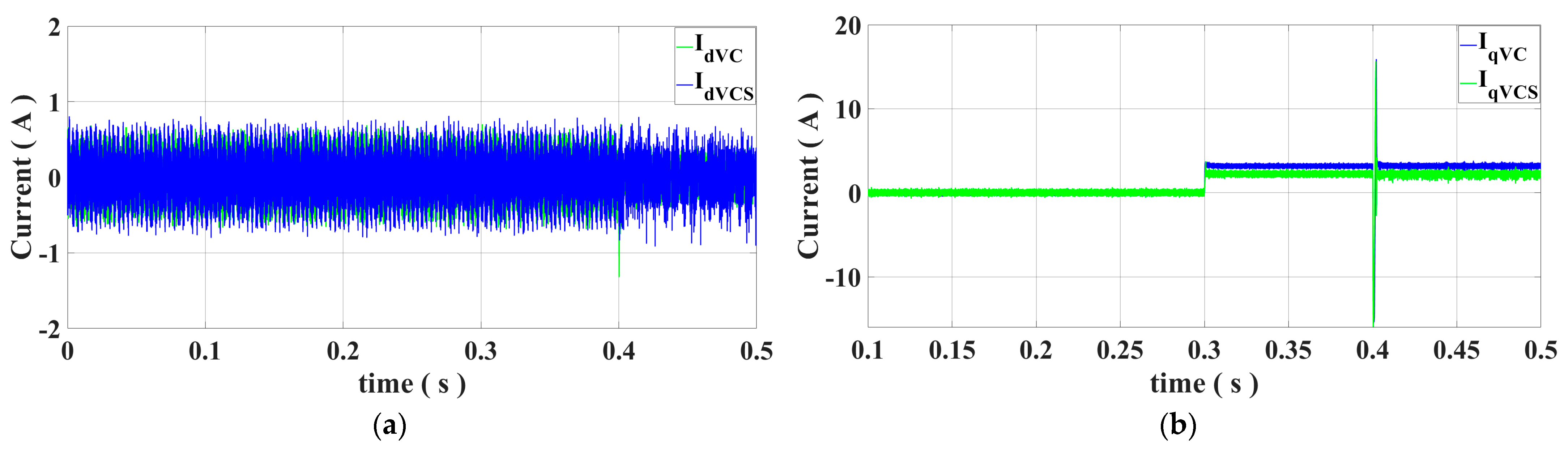
5.1. Analysis of Experimental Results of VC and Sensorless VC

In order to verify the reliability of the proposed sensorless control for sliding-mode observation, it was compared with the VC. The experimental conditions were set as no-load start, and the final speed was set as 1.8 m/s.

According to Figure 10 and Figure 11, by using the sliding-mode observer to control, the motor can start at zero speed, but there is an error in the steady-state speed, and it takes a long time to reach the steady state, and the overshoot is large.

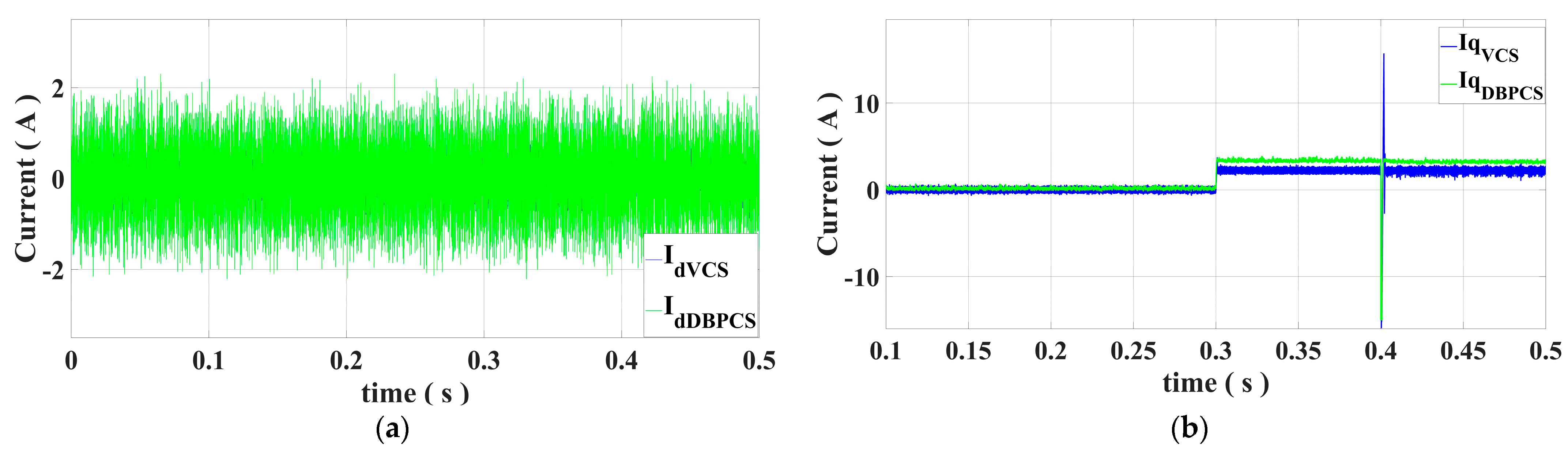
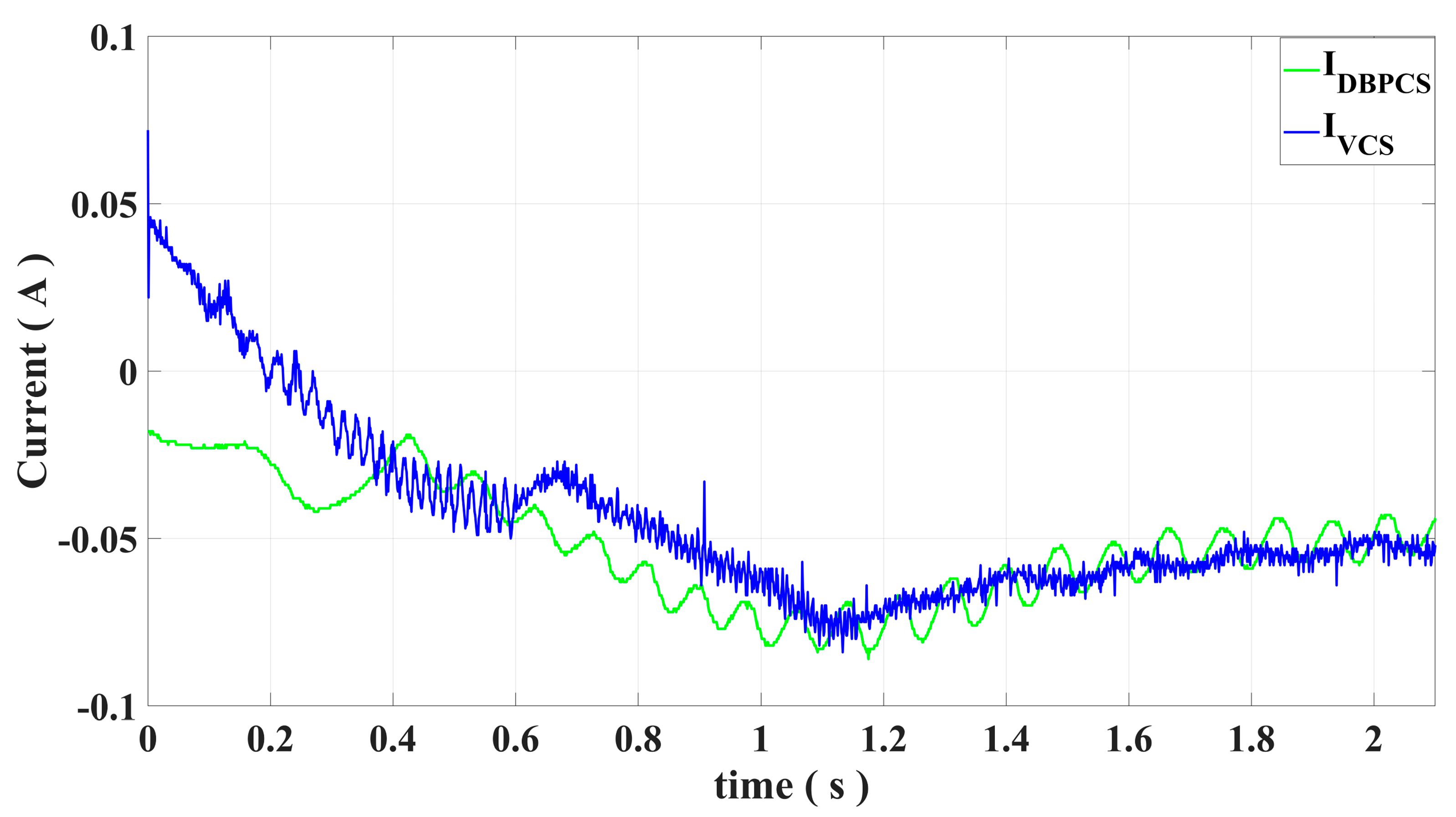
5.2. Analysis of Experimental Results of Sensorless DBPC and Sensorless VC

The experimental conditions were set as no-load start, and the final speed was set as 1.8 m/s. The results are shown in Figure 12, Figure 13 and Figure 14.

The VC and DBPC arrive at a steady state at a similar time, but the DBPC has a better steady-state performance and less fluctuation. Because of outside interference, such as angle estimation and accuracy of the model parameters and environmental noise, the PI controller cannot adapt to the current condition of the adaptive adjustment PI parameters. The DBPC controller’s robustness and anti-interference ability are more robust, so there is less fluctuation at a steady state.

The experimental results show that the DBPCS control method proposed in this paper can achieve better speed estimation. At the same time, the influence of speed fluctuation caused by sliding-mode chattering can be restrained. However, the current fluctuation is large. The reason for the current fluctuation is that there is a delay between the control signal and the error signal. The control signal acting on the current moment is generated according to the error signal of the previous cycle, which makes the deadbeat control strategy ineffective.

6. Conclusions

This paper presents a new predictive current control designed to estimate the speed of the motor. It solves the difficulty of global optimization and tuning of PI parameters, accelerates the time for the system to reach the steady state, and the speed fluctuation is smaller after the steady state. Furthermore, the problem is that speed fluctuation caused by sliding-mode chattering becomes effectively suppressed.

However, from the experimental results, the advantages of deadbeat current predictive control cannot be embodied. The reasons are as follows. First, there is a delayed beat between the control signal and the error signal used to eliminate the error signal. Secondly, sliding-mode chattering exists. Although deadbeat current predictive control can restrain the influence of chattering on motor speed, it still exists.

Therefore, in the future, research will be carried out on how to reduce the impact of beat and how to eliminate the impact of sliding-mode chattering.

References

1. Wu, T.; Lu, K.; Zhu, J.; Lei, G.; Guo, Y.; Tang, W. Calculation of Eddy Current Loss in a Tubular Oscillatory LPMSM Using Computationally Efficient FEA. IEEE Trans. Ind. Electron. 2019, 66, 6200–6209. [Google Scholar] [CrossRef]
2. Wang, B.; Wang, Y.; Feng, L.; Jiang, S.; Wang, Q.; Hu, J. Permanent-Magnet Synchronous Motor Sensorless Control Using Proportional-Integral Linear Observer with Virtual Variables: A Comparative Study with a Sliding Mode Observer. Energies 2019, 12, 877. [Google Scholar] [CrossRef] [Green Version]
3. Cao, F.; An, Q.; Zhang, J.; Zhao, M.; Li, S. Variable Weighting Coefficient of EMF Based Enhanced Sliding Mode Observer for Sensorless PMSM Drives. Energies 2017, 15, 6001. [Google Scholar] [CrossRef]
4. Wu, T.; Feng, Z.; Wu, C.; Lei, G.; Guo, Y.; Zhu, J.; Wang, X. Multiobjective Optimization of a Tubular Coreless LPMSM Based on Adaptive Multiobjective Black Hole Algorithm. IEEE Trans. Ind. Electron. 2019, 67, 3901–3910. [Google Scholar] [CrossRef]
5. Chen, Q.; Xu, G.; Liu, G.; Zhao, W.; Lin, Z.; Liu, L. Torque Ripple Reduction in Five-Phase Interior Permanent Magnet Motors by Lowering Interactional MMF. IEEE Trans. Ind. Electron. 2018, 65, 8520–8531. [Google Scholar] [CrossRef]
6. Zhu, X.; Huang, J.; Quan, L.; Xiang, Z.; Shi, B. Comprehensive Sensitivity Analysis and Multi-Objective Optimization Research of Permanent Magnet Flux-Intensifying Motors. IEEE Trans. Ind. Electron. 2019, 66, 2613–2627. [Google Scholar] [CrossRef]
7. Sun, X.; Hu, C.; Zhu, J.; Wang, S.; Zhou, W.; Yang, Z.; Lei, G.; Li, K.; Zhu, B.; Guo, Y. MPTC for PMSMs of EVs with Multi-Motor Driven System Considering Optimal Energy Allocation. IEEE Trans. Magn. 2019, 55, 8104306. [Google Scholar] [CrossRef]
8. Zhang, Y.; Zhu, J.; Zhao, Z.; Xu, W.; Dorrell, G. An Improved Direct Torque Control for Three-Level Inverter-Fed Induction Motor Sensorless Drive. IEEE Trans. Power Electron. 2012, 27, 1502–1513. [Google Scholar] [CrossRef]
9. Kim, S.; Yoon, I.; Jung, S.; Ko, J. Robust Sensorless Control of Interior Permanent Magnet Synchronous Motor Using Deadbeat Extended Electromotive Force Observer. Energies 2022, 15, 7568. [Google Scholar] [CrossRef]
10. Schroedl, M. Sensorless Control of AC Machines at Low Speed and Standstill Based on the “INFORM” Method. In Proceedings of the Conference Record of the 1996 IEEE Industry Applications Conference Thirty-First IAS Annual Meeting, San Diege, CA, USA, 6–10 October 1996; pp. 270–277. [Google Scholar]
11. Morimoto, S.; Kawamoto, K.; Sanada, M.; Takeda, Y. Sensorless Control Strategy for Salient-Pole PMSM Based on Extended EMF in Rotating Reference Frame. IEEE Trans. Ind. Appl. 2002, 38, 1054–1061. [Google Scholar] [CrossRef]
12. Jiang, Y.; Xu, W.; Mu, C.; Zhu, J.; Dian, R. An Improved Third-Order Generalized Integral Flux Observer for Sensorless Drive of PMSMs. IEEE Trans. Ind. Electron. 2019, 66, 9149–9160. [Google Scholar] [CrossRef]
13. Almarhoon, A.; Zhu, Q.; Xu, P. Improved Rotor Position Estimation Accuracy by Rotating Carrier Signal Injection Utilizing Zero-Sequence Carrier Voltage for Dual Three-Phase PMSM. IEEE Trans. Ind. Electron. 2017, 35, 3767–3776. [Google Scholar] [CrossRef]
14. Tang, Q.; Shen, A.; Luo, X.; Xu, J. PMSM Sensorless Control by Injecting HF Pulsating Carrier Signal into ABC Frame. IEEE Trans. Power Electron. 2017, 32, 3767–3776. [Google Scholar] [CrossRef]
15. Corley, J.; Lorenz, D. Rotor Position and Velocity Estimation for a Salient-Pole Permanent Magnet Synchronous Machine at Standstill and High Speeds. IEEE Trans. Ind. Appl. 1998, 34, 784–789. [Google Scholar] [CrossRef] [Green Version]
16. Cirrincione, M.; Pucci, M. Sensorless Direct Torque Control of an Induction Motor by a TLS-Based MRAS Observer with Adaptive Integration. Automatic 2005, 41, 1843–1854. [Google Scholar] [CrossRef]
17. Gao, W.; Guo, Z. Speed Sensorless Control of PMSM using Model Reference Adaptive System and RBFN. J. Netw. 2013, 8, 213–220. [Google Scholar] [CrossRef]
18. Fadi, A.; Ahmad, A.; Rabia, S.; Cristina, M.; Ibrahim, K. Velocity Sensor Fault-Tolerant Controller for Induction Machine using Intelligent Voting Algorithm. Energies 2022, 15, 3084. [Google Scholar]
19. Zbede, B.; Gadoue, M.; Atkinson, J. Model Predictive MRAS Estimator for Sensorless Induction Motor Drives. IEEE Trans. Ind. Electron. 2016, 63, 3511–3521. [Google Scholar] [CrossRef] [Green Version]
20. Zou, J.; Xu, W.; Zhu, J.; Liu, Y. Low-Complexity Finite Control Set Model Predictive Control With Current Limit for Linear Induction Machines. IEEE Trans. Ind. Electron. 2018, 65, 9243–9254. [Google Scholar] [CrossRef]
21. Khan, A.; Guo, Y.; Zhu, J. Model Predictive Observer Based Control for Single-Phase Asymmetrical T-Type AC/DC Power Converter. IEEE Trans. Ind. Electron. 2019, 55, 2033–2044. [Google Scholar] [CrossRef]
22. Sun, X.; Gao, J.; Lei, G.; Zhu, J. Speed Sensorless Control for Permanent Magnet Synchronous Motors Based on Finite Position Set. IEEE Trans. Ind. Electron. 2020, 67, 6089–6100. [Google Scholar] [CrossRef]
23. Alathamneh, E.; Ghanayem, H.; Yang, X.; Nelms, R. Three-Phase Grid-Connected Inverter Power Control under Unbalanced Grid Conditions Using a Proportional-Resonant Control Method. Energies 2022, 15, 7051. [Google Scholar] [CrossRef]
24. Liu, T.; Chang, K.; Li, J. Design and Implementation of Periodic Control for a Matrix Converter-Based Interior Permanent Magnet Synchronous Motor Drive System. Energies 2021, 14, 8073. [Google Scholar] [CrossRef]
25. Xin, G.; Li, Y.; Chen, W.; Jin, X. Improved Deadbeat Predictive Control Based Current Harmonic Suppression Strategy for IPMSM. Energies 2022, 15, 3943. [Google Scholar]
26. Zeng, X.; Wang, W.; Wang, H. Adaptive PI and RBFNN PID Current Decoupling Controller for Permanent Magnet Synchronous Motor Drives: Hardware- Validated Results. Energies 2022, 15, 6353. [Google Scholar] [CrossRef]
27. Lin, J.; Zhao, Y.; Zhang, P.; Wang, J.; Su, H. Research on Compound Sliding Mode Control of a Permanent Magnet Synchronous Motor in Electromechanical Actuators. Energies 2021, 14, 7293. [Google Scholar] [CrossRef]
Figure 1. The speed comparison diagram between VC and VCS.
Energies 16 00628 g001
Figure 2. Speed error, using SMO.
Energies 16 00628 g002
Figure 3. Comparison diagram of id,q. (a) The id comparison diagram between VC and VCS. (b) The iq comparison diagram between VC and VCS.
Energies 16 00628 g003
Figure 4. The estimated angles comparison diagram between VC and VCS.
Energies 16 00628 g004
Figure 5. Complete control structure.
Energies 16 00628 g005
Figure 6. Estimated speed used in DBPCS.
Energies 16 00628 g006
Figure 7. Comparison diagram of i d , q . (a) The i d comparison diagram between VCS and DBPCS. (b) The i q comparison diagram between VCS and DBPCS.
Energies 16 00628 g007
Figure 8. Diagram of LPMSM control system.
Energies 16 00628 g008
Figure 9. Diagram of laboratory.
Energies 16 00628 g009
Figure 10. Comparison diagram of speed between VC and VCS.
Energies 16 00628 g010
Figure 11. Comparison diagram of angle.
Energies 16 00628 g011
Figure 12. Comparison diagram of speed.
Energies 16 00628 g012
Figure 13. Comparison diagram of d-axis current.
Energies 16 00628 g013
Figure 14. Comparison diagram of q-axis current.
Energies 16 00628 g014