Abstract
According to the inherent characteristics of the hydraulic power take-off (PTO) system, the output power of a generator tends to be intermittent when the wave is random. Therefore, this paper aims to improve the effective utilization of wave energy and reduce power intermittency by constructing a topology with two branches to transmit electrical energy. Firstly, the wave-to-wire (W2W) model of the system is constructed. Secondly, the W2W model is simulated by using synovial and quasi-proportional resonance (QPR) control with regular and irregular incident waves, and the results of PI control are compared. Then, the control strategy in simulation is verified by experiments. The simulation and experimental results show that the control strategy has better performance, and the stability of the system output power is greatly improved.
1. Introduction
Nowadays, the global energy demand has increased significantly, and in order to reduce the exploitation of limited fossil energy, countries are trying to develop new energy industries to promote smart energy [1]. The ocean, which covers 71% of the Earth’s surface area, is a treasure house of green energy. It contains a large amount of energy, and wave energy is considered to be one of the most promising ocean energy sources, so it has received a great deal of attention and research [2,3]. Although wave energy has the advantages of large storage capacity, high energy density, and green and clean attributes [4,5], the complexity of the ocean environment and the randomness of waves in time and space also make the acquisition of wave energy challenging [6,7,8].
In recent years, the efforts of researchers have led to the development of hundreds of wave energy converters (WEC) [9], many of which have been applied in practice [10]. According to the way of capturing wave energy, most WECs can be categorized as oscillating water column type [11,12,13], oscillating body type [14], and overtopping type [15,16], among which the oscillating body type is most widely used. Oscillating body type is characterized by the relative motion between a single body and the seabed or multiple bodies under the action of waves, converting wave energy into kinetic energy of the body and later converting kinetic energy into electrical energy by the energy-transfer mechanism. Single floating body type, also known as point absorption type, is the simplest type of oscillating wave generator [17,18]. The oscillating body mainly includes two kinds of energy transfer mechanisms: one is the direct-drive power take-off (PTO), and the other is the hydraulic PTO, which are described in [19]. The direct-drive PTO uses wave absorption float motion to drive the reciprocating linear motion of the generator, and the generator directly converts the captured wave energy into electrical energy [20]. In contrast, the HPTO has an additional intermediate energy storage link than the direct-drive PTO and thus has the characteristics of three-stage energy conversion. At the same time, because the accumulator realizes wave and generator decoupling, there is no maximum power point in the hydraulic energy storage wave power-generation system. Therefore, it is not possible to achieve the maximum power output of the system by controlling the speed of the generator. From the obtained research results, it is clear that the hydraulic PTO can better adapt to the randomness of wave energy variation, which can improve the power quality [21]. Thus far, many scholars have conducted extensive research direct-drive PTO and hydraulic PTO, respectively. In [22], the application of a linear permanent magnet generator in direct-drive PTO was summarized and compared comprehensively, along with numerical and experimental analyses. In [23], the nonlinear model prediction method was introduced to direct-drive PTO, and the optimal damping of a permanent magnet linear generator was experimentally investigated under the guidance. The connection between the average output power of the direct-drive PTO, the intrinsic impedance, and the equivalent impedance of the generator was discussed in [24], and the maximum power point tracking was realized based on the hill-climbing method. The application of hydraulic PTO technology in WEC was reviewed in [25], and a novel wave-plus-photon hybrid WEC structure combined with solar cell technology was proposed. In [26], the composition of the hydraulic PTO and various control strategies were introduced in detail, and the advantages and disadvantages were also discussed. The concept of oil–hydraulic power take-off was proposed in [27], and the use of a hydraulic transformer in the hydraulic PTO was confirmed to be beneficial by simulation analysis of three sea conditions.
Currently, the main focus in research on WEC is to improve wave absorption efficiency, while some other studies also consider all components from wave to the grid, also known as W2W models. In [28], an optimization procedure was developed to find the optimal resistive loading of the WEC under irregularly incident waves and was studied based on developed W2W models, which showed a significant increase in the power-generation capacity of the device. A high-fidelity model with generality was proposed in [29]. The comparison between the constant pressure hydraulic PTO model and the variable pressure model shows that the efficiency of the WEC is not necessarily proportional to the power generation. In [30], a fully coupled time-domain model based on the hydrodynamic, mechanical and electrical response of the WEC was constructed, which can be used to monitor the interactions among the devices in the WEC and respond to wave state or grid emergencies. Numerical simulation and experimental research on W2W models were mainly introduced in [31].
In this paper, in order to reduce the power intermittency in the wave power-generation system based on hydraulic PTO, a two-branch power-generation topology is constructed, as shown in Figure 1. Simulations and experiments show that the two generators can effectively improve the utilization of wave energy and extend the operating time of the whole system through reasonable coordination. In addition, this paper makes a general comparison with some other references in terms of system output power, as shown in Table 1. This paper is organized as follows. Section 2 presents the mathematical model of the PTO system in the W2W model in detail. Section 3 shows the control block diagram of the wave power system and provides a detailed description of the control strategy. Section 4 presents a simulation study of the wave power system under regular and irregular incident waves. Section 5 provides experimental validation of the simulation. Conclusions are given in Section 6.

Figure 1.
Double-branch hydraulic energy storage wave power-generation system.

Table 1.
Comparison of system output power.
2. Mathematical Model of Hydraulic PTO System
The hydraulic PTO system mainly includes a hydraulic cylinder, check valve, accumulator, and hydraulic motor. The working principle is as follows: the rod cavity and rodless cavity of the hydraulic cylinder work alternately under the action of the wave energy absorber, and the hydraulic oil in the compressed tank enters the accumulator, converting mechanical energy into hydraulic energy stored in the accumulator. When the pressure in the accumulator reaches the set value, the hydraulic autonomy system controls the hydraulic valve to open, and the hydraulic oil with high pressure impacts the hydraulic motor, which drives the generator to generate electricity to realize the conversion of hydraulic energy into electrical energy. The specific implementation of the hydraulic PTO system in the simulation is as follows: the waves simulated by the wave spectrum are used as velocity signals to produce the hydraulic cylinder motion, and the flow through the accumulator is simultaneously calculated based on the motion model of the hydraulic cylinder. The flow through the accumulator minus the flow of the hydraulic motor is the final flow into the accumulator. The pressure value in the accumulator is calculated from the inflow, and this pressure value is used to control the start and stop of the generator.
In addition, it is important to note that in order to ensure the safety of the system, when extreme sea conditions lead to excessive pressure in the accumulator, the system must stop working and stabilize itself with the mooring system.
2.1. Mathematical Model of Hydraulic Cylinder
The double acting hydraulic cylinder has hydraulic fluid between both chambers, providing hydraulic fluid transfer in both directions.
where is the flow rate of the rod chamber, is the flow rate of the rodless chamber, is the movement speed of the hydraulic rod, is the diameter of the hydraulic cylinder, and is the piston rod diameter.
2.2. Mathematical Model of the Bladder-Type Accumulator
The structure of the hydraulic accumulator is bladder type, which is mainly composed of an air chamber and a liquid chamber. The working principle is that if the fluid pressure at the inlet of the accumulator is higher than the pressure of the internal air chamber, the fluid will enter the accumulator and compress the air chamber, thus storing energy. During the power-generation process, the accumulator uses the compression and expansion of the air in the air chamber to store and release the hydraulic energy. According to Boyle’s gas law, the relationship between pressure and volume is as follows:
where is the pressure, is the volume of the gas, and is the variable process index of the gas, which is 1.4 for the adiabatic process and 1 for the isothermal process; is a constant.
During the operation of the system, the accumulator can be considered to be working in an isothermal state, so the gas in the gas chamber of the accumulator satisfies the following equation:
where is the volume of the accumulator, is the gas chamber pre-charge pressure, is the standard atmospheric pressure, is the volume of hydraulic fluid in the liquid chamber, and is the pressure of the accumulator.
The hydraulic flow in the accumulator is expressed as follows:
2.3. Mathematical Model of Hydraulic Motor
The hydraulic motor is an important energy-conversion element to convert hydraulic energy into electrical energy in the hydraulic power-generation system. It requires fast working speed and high reliability, so the axial piston-type quantitative motor is used. In addition, the quantitative motor has a fixed displacement and does not need an additional control unit, which also avoids the failure of the control circuit of the variable motor. The flow rate and output torque of the hydraulic motor are expressed, respectively, as follows:
where is the displacement of the hydraulic motor, is the hydraulic motor speed, is the hydraulic motor leakage coefficient, is the hydraulic motor inlet and outlet pressure difference and, in the whole power-generation process, can be approximated as . is the hydraulic motor mechanical efficiency, and is the hydraulic motor volume efficiency.
3. Control Strategy of Hydraulic Storage Wave Power-Generation System
The control block diagram is shown in Figure 2, where the * represents the reference value. The speed outer loop and current inner loop on the generator side are controlled by sliding mode control (SMC)and QPR control, respectively, where the reference value of speed uses the optimal pressure-speed curve [32], as shown in Equation (8). The grid side uses the voltage outer loop and QPR-controlled current inner loop to realize grid-connected unit power factor control.
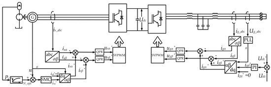
Figure 2.
Control block diagram of hydraulic storage wave power-generation system.
3.1. PR Control
PR control is based on the inner membrane principle, and structurally, it was developed by introducing two poles on the imaginary axis of the PI controller transfer function, which can be expressed as follows:
where is the proportional gain, is the integral gain, and is the angular frequency.
Ideally, the amplitude gain of the PR controller resonance at the two poles tends to infinity, thus achieving zero steady-state tracking for a given quantity. Compared with PI controller, PR controller can realize the tracking of AC signal, and the control system does not contain a feedforward compensation and decoupling term related to motor parameters, which reduces coordinate transformation, so it reduces the difficulty of implementing the control algorithm and improves the robustness of the system. Moreover, it has much larger gain at the fundamental frequency than PI, so the steady-state error is smaller. However, the ideal PR control is difficult to implement in digital systems because its narrow frequency gain bandwidth will lead to poor immunity to interference, poor dynamic stability, and a relatively significant drop in gain beyond the resonance point. Therefore, quasi-QPR control is introduced, and its transfer function is expressed as follows:
where is the cut-off frequency of the QPR controller.
From the transfer function, QPR control introduces to PR control, for which the gain at the resonance point is not as high as PR control but also has a very high amplitude and still has a good tracking performance. In addition, the presence of broadens the bandwidth of the resonant frequency gain and reduces the impact due to frequency shift, thus improving the dynamic performance of the system.
3.2. Design of QPR Controller
From Equation (10), the QPR controller needs to design three parameters. Determining the appropriate , , and through the design can push the system stability and anti-interference ability to their most optimal levels. In this paper, the bode diagram of the amplitude-frequency and phase-frequency characteristics of the QPR controller when each parameter is varied is obtained using the control variable method, as shown in Figure 3.
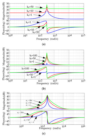
Figure 3.
Bode diagram of QPR when , , and change. (a) change; (b) change; (c) change.
It can be seen from Figure 3 that when only is changed, the bandwidth of controller and the amplitude at the fundamental frequency do not increase much, while the amplitude outside the frequency band increases with the increase of , which means that mainly affects the amplitude outside the frequency band. When only is changed, the bandwidth of controller and the gain at the fundamental frequency increase with the increase of , while the amplitude gain outside the frequency band basically remains unchanged, which means that mainly affects the bandwidth of the controller and the gain at the fundamental frequency. When only is changed, the bandwidth of the controller increases with the increase of , while the amplitude outside the frequency band and the amplitude at the fundamental frequency basically remain unchanged, which indicates that has good selectivity to the signal and mainly determines the bandwidth of the controller.
In order to facilitate the QPR control to be implemented programmatically, it needs to be discretized. In this paper, Tustin is used for discretization, and the discretization transformation equation is shown below:
Substituting Equation (11) into Equation (10), the difference equation for the QPR controller can be solved as follows:
The controller can be controlled using the differential equation.
4. Analysis of Simulation Results under Regular and Irregular Incident Waves
The simulation parameters of the system mainly include the permanent magnet synchronous motor, accumulator, hydraulic cylinder, hydraulic motor and line, etc. The specific values are given in Table 2.
Table 2.
System Simulation Parameters.
4.1. Waves Spectrum
Waves can be generated by a variety of factors, but usually the dominant force is wind waves, which are generated by the wind blowing across the surface of the sea. In order to describe fluctuations more accurately, there are several commonly used spectra, such as the JONSWAP spectrum, the Wallops spectrum, the Pierson–Moskowitz spectrum, and the Bretschneider spectrum, etc. Among them, JONSWAP spectrum and Pierson–Moskowitz spectrum are more widely used. For well-developed oceans with sufficiently long wind distances, the Pierson–Moskowitz spectrum is generally used. For limited wind distance, the JONSWAP spectrum is more recommended.
In this paper, the JONSWAP is used for the study. The JONSWAP spectrum can be expressed by the following equation:
where is the effective wave height, is the spectral peak period, is the spectral peak factor, and is the peak shape parameter.
Figure 4 shows the JONSWAP spectrum for waves with a spectral peak period of 6 s and an effective wave height of 1.2 m.
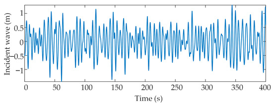
Figure 4.
The incident wave with a spectral peak period of 6 s and an effective wave height of 1.2 m.
4.2. Analysis of Simulation Results under Regular Incident Waves
Based on the linear theory, the simplified JONSWAP spectrum of the SIN function is used to simulate the regular incident wave under stable wave condition within 60 s, as shown in Figure 5, and is used as the input to the hydraulic cylinder. Figure 6 shows the pressure variation of the accumulator under regular incident waves. From Figure 6, it is seen that the hydraulic control valves are all in the open-valve state due to the high initial accumulator pressure, at which time the two hydraulic motors drive the two generators (i.e., G1 and G2) to work, respectively. The accumulator receives the energy transferred from the mechanical work of the hydraulic cylinder and at the same time provides energy to support the hydraulic motor to drive the generator to generate electricity so as to realize the conversion of mechanical energy to hydraulic energy to electrical energy. When the energy provided by the hydraulic cylinder is less than the total energy consumed by the operation of G1 and G2, the accumulator pressure starts to drop. After 20 s, when the accumulator pressure drops to the preset closing pressure (i.e., 11 MPa) of the hydraulic control valve of G1, G1 stops working, and the speed is reduced to zero by the braking resistor connected to the system. At this point, G1 enters an intermittent power-generation state and waits for the next generation cycle. When G1 stops working, the output energy of the hydraulic cylinder is greater than the energy consumed by G2, the pressure of the accumulator will rise slowly, and because the accumulator pressure is always greater than the closing pressure of the hydraulic control valve of G2, G2 is always in working condition.
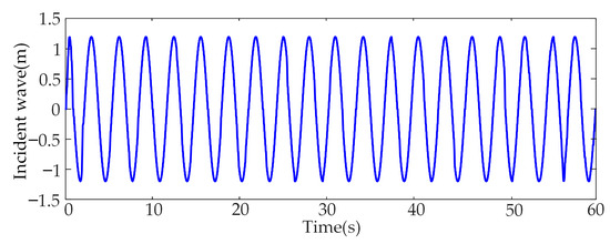
Figure 5.
Regular incident waves.
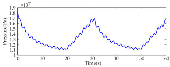
Figure 6.
Accumulator pressure under regular incident waves.
During the entire power-generation process, the operating speed of G1 and G2 follows the set optimal pressure-velocity curve, as shown in Figure 7 and Figure 8. The difference is that the velocity outer loop in Figure 7 is controlled by PI, while Figure 8 is controlled by SMC. In Figure 7, the speed overshoot is 16.6%, and the dynamic response time is 0.05 s, while in Figure 8, the overshoot of speed is 1.3%, the response time is 0.04 s without steady-state error. From the control effect of SMC and PI, it can be seen that the SMC control has better performance.
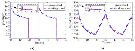
Figure 7.
Speed under PI control. (a) Speed of G1; (b) speed of G2.
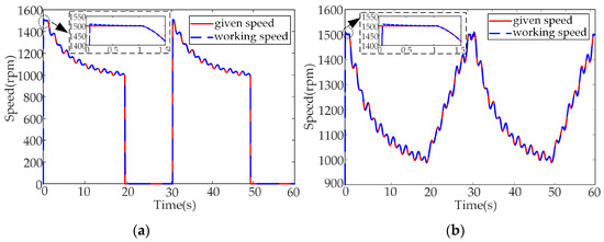
Figure 8.
Speed under SMC control. (a) Speed of G1; (b) speed of G2.
The power curves of G1 and G2 are shown in Figure 9, and it can be seen from Equation (7) that the power is directly related to the accumulator pressure. When the power drops to about 40% of the rated power, G1 stops working. By shutting down G1 in time to slow down the consumption of wave energy, the operating time of G2 is increased. This extends the operating time of the system, keeping the system in a generatable power state and maintaining critical system load demand. The voltage and current of G1 and G2 are shown in Figure 10 and Figure 11. The voltage waveform is for the complete simulation period, and the current is 1 s. As shown in Figure 10, the trend of voltage variation is similar to the speed curve throughout the generation process. In addition, it can be seen from the current waveform that the current dynamic response time is about 0.075 s under the regular incident waves.
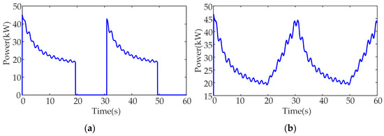
Figure 9.
Power Curve. (a) Power of G1; (b) power of G2.
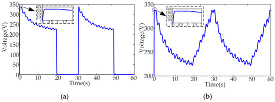
Figure 10.
The phase voltage waveforms under regular incident waves. (a) Phase voltage of G1; (b) phase voltage of G2.
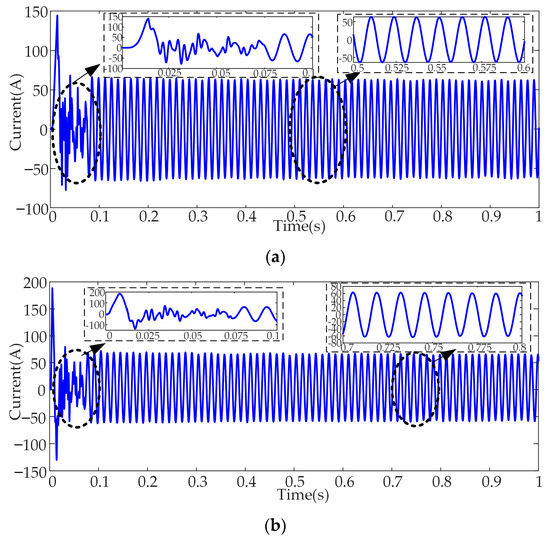
Figure 11.
The phase current waveforms under regular incident waves. (a) Phase current of G1; (b) phase current of G2.
Figure 12 shows the active and reactive power curves of the grid connection. From Figure 12, the grid-connected reactive power is zero, and the unit factor power control is realized. Meanwhile, it can be seen from the figure that the whole system has been in the state of transferring power to the outside, which greatly improves the intermittent power generation due to the work of a single generator, thus improving the stability of the system power supply. Figure 13 shows the bus voltage curve, from which it can be seen that the bus voltage can reach the given value and remain stable within a short time after the system starts working, and the fluctuation range does not exceed 1 V. Figure 14 shows the FFT analysis of the grid-connected current, where PI control is used for the current inner loop in Figure 14a and QPR control in Figure 14b. It can be seen from Figure 14 that the total harmonic distortion rate after QPR control is 0.87% lower than that of PI control, and the amplitude of higher harmonics is effectively reduced, which is sufficient to demonstrate the superiority of QPR control.
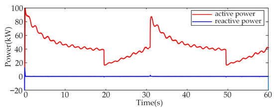
Figure 12.
Grid-connected active and reactive power.
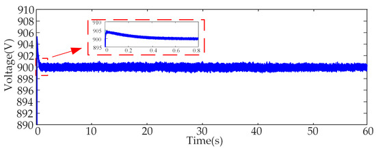
Figure 13.
DC bus voltage under regular incident waves.
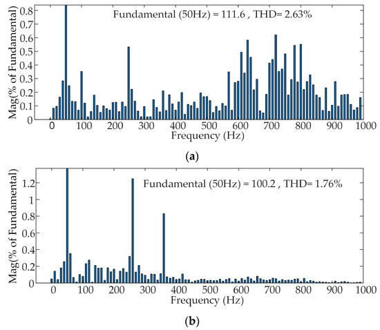
Figure 14.
FFT analysis of grid-connected currents. (a) FFT under PI control; (b) FFT under QPR control.
4.3. Analysis of Simulation Results under Irregular Incident Waves
To better fit the actual situation, a combination of large, medium, and small waves was used to simulate irregular incident waves by changing the effective wave height and frequency of the JONWAP spectrum. The first 30 s are large waves with an effective wave height of 2.4 m, the middle 40 s are medium waves with an effective wave height of 1.2 m, and the last 20 s are small waves with an effective wave height of 0.5 m, as shown in Figure 15. Under the irregular incident waves, the accumulator pressure is shown in Figure 16. For the whole system, from the energy point of view, the input energy is greater than the energy consumed by G1 and G2 due to the continuous input of large waves in the first 30 s, resulting in a rising pressure of the accumulator. At this point, if the pressure exceeds the maximum safety pressure of the accumulator, the measures to protect the accumulator should be started immediately to prevent damage to the system. During the first 30 s of the medium waves, the input energy is less than the energy consumed by the generators, at which point the accumulator pressure begins to drop. Since both generators are equipped with larger displacement hydraulic motors, the pressure drop is more obvious, and in about 60 s drop to the hydraulic motor shut-off pressure of G1, G1 stops working.
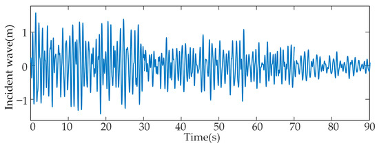
Figure 15.
Irregular incident waves.
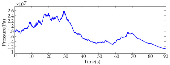
Figure 16.
Accumulator pressure under irregular incident waves.
Afterwards, during the last 10 s of the medium waves, although only G2 was working alone, the accumulator pressure did not rise to the open-valve pressure of the hydraulic motor of G1, so G1 was in a continuous off state. In the case of small waves, the input energy still is less than the energy consumed by G2 working, the accumulator pressure still drops, and eventually, G2 stops working around 85 s because the energy of the wave is too small. During the whole operation, the speed curves of G1 and G2 are shown in Figure 17. It can be seen from Figure 17 that the overshoot of speed is very small, the dynamic response is fast, and there is no steady-state error, which also shows the superiority of the control strategy in this paper.
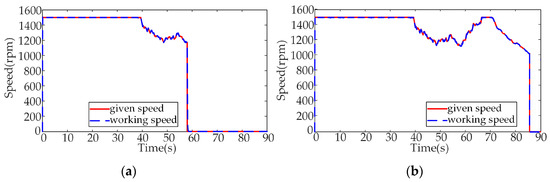
Figure 17.
Speed curves. (a) Speed of G1; (b) speed of G2.
Figure 18 shows the DC bus voltage under irregular incident waves, and it can be seen that the voltage reaches the given value in about 0.4 s, and the steady-state amplitude fluctuates within plus or minus 2 V. The power curves are shown in Figure 19. Figure 19 shows that the power of the two generators follows the accumulator pressure before they stop working. During the medium waves phase, the operating time during the small-wave period is extended by turning off G1 in time to prevent the whole system from stopping immediately just after entering the small-wave period. Finally, during the small-wave phase, G2 stops working due to the lack of wave energy. The voltage and current of G1 and G2 are shown in Figure 20 and Figure 21. The voltage waveforms have similar characteristics to those under the regular incident waves, and both are similar to the speed curve. Further, the dynamic response time of the current is 0.1 s, which is 0.025 s more than that under the regular incident waves. The grid-connected power of the whole system is shown in Figure 22, and the unit power factor control is realized.
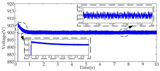
Figure 18.
DC bus voltage under irregular incident waves.
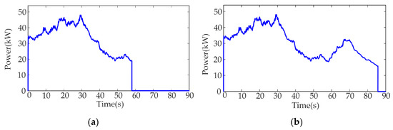
Figure 19.
Power curves. (a) Power of G1; (b) power of G2.
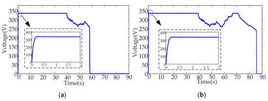
Figure 20.
The phase voltage waveforms under irregular incident waves. (a) Phase voltage of G1; (b) phase voltage of G2.
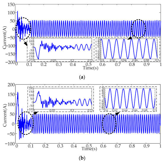
Figure 21.
The phase current waveforms under irregular incident waves. (a) Phase current of G1; (b) phase current of G2.
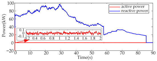
Figure 22.
Grid-connected power.
5. Experimental Analysis
The experimental platform is shown in Figure 23, mainly using the upper computer, RT-LAB, and oscilloscope for experiments, and the experimental parameters are kept consistent with the simulation parameters.
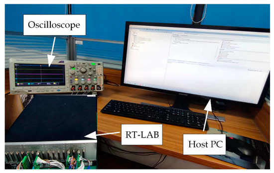
Figure 23.
Experimental platform.
Figure 24 shows the speed and power curves of the two generators under regular incident waves, with G1 curve at the top and G2 curve at the bottom. From the Figure 24a, it can be seen that the overshoot of the speed of both generators at start-up does not exceed 100 rpm, and they can operate stably throughout the working time. From the Figure 24b, it can be seen that G1 has been generating intermittently during the whole working time, but the presence of G2 has kept the whole system in working condition through reasonable cooperation. The waveforms of speed and power of both generators are basically consistent with the simulation analysis, which also verifies the effectiveness of the control strategy in the simulation.
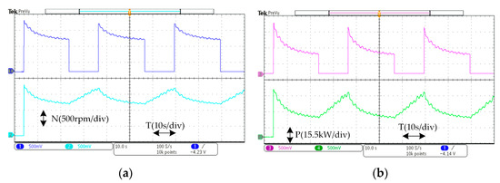
Figure 24.
Speed and power curves of G1 and G2 under regular waves. (a) Speed curve of G1 and G2; (b) power curve of G1 and G2.
Figure 25 shows the speed and power curves of the two generators under irregular waves. From Figure 25a, it can be seen that the speeds of both generators are stable at 1500 rpm during large waves and then change with the pressure value of the accumulator during medium and small waves until they stop working. From Figure 25b, it can be seen that the power of both generators increases with the increase of wave energy during large waves; during the medium wave, the power shows a decreasing trend, and at the end of medium waves, G1 stops working. During small waves, the earlier shutdown of G1 slows down the consumption of wave energy, allowing G2 to remain operational for some time during small waves. The analysis of the whole simulation process can also be verified in the experiment.
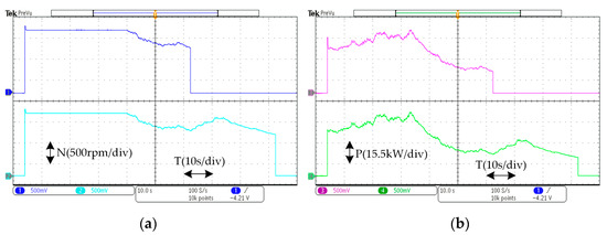
Figure 25.
Speed and power curves of G1 and G2 under irregular waves. (a) Speed curve of G1 and G2; (b) power curve of G1 and G2.
6. Conclusions
This paper proposes a new hydraulic storage wave energy-generation topology with two branches to transmit electrical energy and conducts simulations and experimental research. The simulation results show that reasonable coordination of the operation time of G1 and G2 according to the magnitude of wave and accumulator pressure can effectively improve the utilization of wave energy and reduce the intermittency of the system output power. In addition, compared with PI control, the control strategy used in this paper reduces the speed overshoot by 15% and the harmonic distortion rate of current by 0.87%.
The simulation verifies that the power-generation characteristics of the system are essentially the same under regular and irregular incident waves. This implies that the hydraulic energy-conversion system can convert the unstable wave energy into stable electrical energy, thus also improving the power-generation quality.
Author Contributions
Conceptualization, Z.L.; methodology, W.H.; investigation, S.L.; resources, S.L.; writing—original draft preparation, W.H.; writing—review and editing, X.W., C.S.L. and Y.Y. All authors have read and agreed to the published version of the manuscript.
Funding
This work was supported by the National Key Research and Development Plan of China (Project Number 2019YFB1504404).
Institutional Review Board Statement
Not applicable.
Informed Consent Statement
Not applicable.
Data Availability Statement
Not applicable.
Conflicts of Interest
The authors declare no conflict of interest.
References
- Lai, C.S.; Lai, L.L.; Lai, Q.H. Smart Energy for Transportation and Health in a Smart City; IEEE Press/Wiley: Piscataway, NJ, USA, 2022. [Google Scholar]
- Zhang, Y.; Zhao, Y.; Sun, W.; Li, J. Ocean wave energy converters: Technical principle, device realization, and performance evaluation. Renew. Sustain. Energy Rev. 2021, 141, 110764. [Google Scholar] [CrossRef]
- Wang, C.-N.; Thanh, N.; Su, C.-C. The Study of a Multicriteria Decision Making Model for Wave Power Plant Location Selection in Vietnam. Processes 2019, 7, 650. [Google Scholar] [CrossRef]
- Khojasteh, D.; Mousavi, S.M.; Glamore, W.; Iglesias, G. Wave energy status in Asia. Ocean Eng. 2018, 169, 344–358. [Google Scholar] [CrossRef]
- Lehmann, M.; Karimpour, F.; Goudey, C.A.; Jacobson, P.T.; Alam, M.-R. Ocean wave energy in the United States: Current status and future perspectives. Renew. Sustain. Energy Rev. 2017, 74, 1300–1313. [Google Scholar] [CrossRef]
- Aderinto, T.; Li, H. Ocean Wave Energy Converters: Status and Challenges. Energies 2018, 11, 1250. [Google Scholar] [CrossRef]
- Haces-Fernandez, F.; Li, H.; Ramirez, D. Analysis of Wave Energy Behavior and Its Underlying Reasons in the Gulf of Mexico Based on Computer Animation and Energy Events Concept. Sustainability 2022, 14, 4687. [Google Scholar] [CrossRef]
- Soukissian, T.H.; Karathanasi, F.E. Joint Modelling of Wave Energy Flux and Wave Direction. Processes 2021, 9, 460. [Google Scholar] [CrossRef]
- Babarit, A. A database of capture width ratio of wave energy converters. Renew. Energy 2015, 80, 610–628. [Google Scholar] [CrossRef]
- Aderinto, T.; Li, H. Review on Power Performance and Efficiency of Wave Energy Converters. Energies 2019, 12, 4329. [Google Scholar] [CrossRef]
- Elhanafi, A.; Macfarlane, G.; Fleming, A.; Leong, Z. Experimental and numerical investigations on the hydrodynamic performance of a floating–moored oscillating water column wave energy converter. Appl. Energy 2017, 205, 369–390. [Google Scholar] [CrossRef]
- Sheng, W.; Lewis, A. Power Takeoff Optimization to Maximize Wave Energy Conversions for Oscillating Water Column Devices. IEEE J. Ocean. Eng. 2018, 43, 36–47. [Google Scholar] [CrossRef]
- Wang, C.; Zhang, Y. Hydrodynamic performance of an offshore Oscillating Water Column device mounted over an immersed horizontal plate: A numerical study. Energy 2021, 222, 119964. [Google Scholar] [CrossRef]
- Rosa-Santos, P.; Taveira-Pinto, F.; Rodríguez, C.A.; Ramos, V.; López, M. The CECO wave energy converter: Recent developments. Renew. Energy 2019, 139, 368–384. [Google Scholar] [CrossRef]
- Contestabile, P.; Crispino, G.; Di Lauro, E.; Ferrante, V.; Gisonni, C.; Vicinanza, D. Overtopping breakwater for wave Energy Conversion: Review of state of art, recent advancements and what lies ahead. Renew. Energy 2020, 147, 705–718. [Google Scholar] [CrossRef]
- Martins, J.C.; Goulart, M.M.; Gomes, M.d.N.; Souza, J.A.; Rocha, L.A.O.; Isoldi, L.A.; dos Santos, E.D. Geometric evaluation of the main operational principle of an overtopping wave energy converter by means of Constructal Design. Renew. Energy 2018, 118, 727–741. [Google Scholar] [CrossRef]
- Zhang, X.; Tian, X.; Xiao, L.; Li, X.; Chen, L. Application of an adaptive bistable power capture mechanism to a point absorber wave energy converter. Appl. Energy 2018, 228, 450–467. [Google Scholar] [CrossRef]
- Ropero-Giralda, P.; Crespo, A.J.C.; Tagliafierro, B.; Altomare, C.; Domínguez, J.M.; Gómez-Gesteira, M.; Viccione, G. Efficiency and survivability analysis of a point-absorber wave energy converter using DualSPHysics. Renew. Energy 2020, 162, 1763–1776. [Google Scholar] [CrossRef]
- Ahamed, R.; McKee, K.; Howard, I. Advancements of wave energy converters based on power take off (PTO) systems: A review. Ocean Eng. 2020, 204, 107248. [Google Scholar] [CrossRef]
- Faiz, J.; Nematsaberi, A. Linear electrical generator topologies for direct-drive marine wave energy conversion—An overview. IET Renew. Power Gener. 2017, 11, 1163–1176. [Google Scholar] [CrossRef]
- Nam, J.W.; Sung, Y.J.; Cho, S.W. Effective Mooring Rope Tension in Mechanical and Hydraulic Power Take-Off of Wave Energy Converter. Sustainability 2021, 13, 9803. [Google Scholar] [CrossRef]
- Ahamed, R.; McKee, K.; Howard, I. A Review of the Linear Generator Type of Wave Energy Converters’ Power Take-Off Systems. Sustainability 2022, 14, 9936. [Google Scholar] [CrossRef]
- Son, D.; Yeung, R.W. Real-time implementation and validation of optimal damping control for a permanent-magnet linear generator in wave energy extraction. Appl. Energy 2017, 208, 571–579. [Google Scholar] [CrossRef]
- Xiao, X.; Huang, X.; Kang, Q. A Hill-Climbing-Method-Based Maximum-Power-Point-Tracking Strategy for Direct-Drive Wave Energy Converters. IEEE Trans. Ind. Electron. 2016, 63, 257–267. [Google Scholar] [CrossRef]
- Prasad, K.A.; Chand, A.A.; Kumar, N.M.; Narayan, S.; Mamun, K.A. A Critical Review of Power Take-Off Wave Energy Technology Leading to the Conceptual Design of a Novel Wave-Plus-Photon Energy Harvester for Island/Coastal Communities’ Energy Needs. Sustainability 2022, 14, 2354. [Google Scholar] [CrossRef]
- Jusoh, M.A.; Ibrahim, M.Z.; Daud, M.Z.; Albani, A.; Mohd Yusop, Z. Hydraulic Power Take-Off Concepts for Wave Energy Conversion System: A Review. Energies 2019, 12, 4510. [Google Scholar] [CrossRef]
- Gaspar, J.F.; Calvário, M.; Kamarlouei, M.; Guedes Soares, C. Power take-off concept for wave energy converters based on oil-hydraulic transformer units. Renew. Energy 2016, 86, 1232–1246. [Google Scholar] [CrossRef]
- Wang, L.; Lin, M.; Tedeschi, E.; Engström, J.; Isberg, J. Improving electric power generation of a standalone wave energy converter via optimal electric load control. Energy 2020, 211, 118945. [Google Scholar] [CrossRef]
- Penalba, M.; Ringwood, J.V. A high-fidelity wave-to-wire model for wave energy converters. Renew. Energy 2019, 134, 367–378. [Google Scholar] [CrossRef]
- Forehand, D.I.M.; Kiprakis, A.E.; Nambiar, A.J.; Wallace, A.R. A Fully Coupled Wave-to-Wire Model of an Array of Wave Energy Converters. IEEE Trans. Sustain. Energy 2016, 7, 118–128. [Google Scholar] [CrossRef]
- Wang, L.; Isberg, J.; Tedeschi, E. Review of control strategies for wave energy conversion systems and their validation: The wave-to-wire approach. Renew. Sustain. Energy Rev. 2018, 81, 366–379. [Google Scholar] [CrossRef]
- Wang, K.; Sheng, S.; Zhang, Y.; Ye, Y.; Jiang, J.; Lin, H.; Huang, Z.; Wang, Z.; You, Y. Principle and control strategy of pulse width modulation rectifier for hydraulic power generation system. Renew. Energy 2019, 135, 1200–1206. [Google Scholar] [CrossRef]


Disclaimer/Publisher’s Note: The statements, opinions and data contained in all publications are solely those of the individual author(s) and contributor(s) and not of MDPI and/or the editor(s). MDPI and/or the editor(s) disclaim responsibility for any injury to people or property resulting from any ideas, methods, instructions or products referred to in the content. |
© 2023 by the authors. Licensee MDPI, Basel, Switzerland. This article is an open access article distributed under the terms and conditions of the Creative Commons Attribution (CC BY) license (https://creativecommons.org/licenses/by/4.0/).