Adaptive Mixed-Integer Linear Programming-Based Energy Management System of Fast Charging Station with Nuclear–Renewable Hybrid Energy System

Abstract

The concept of transportation electrification is proliferating due to its high impact on emission reduction. However, the increased usage of electric vehicles strains the power grid’s charging infrastructure. As a result, to reduce demand on the power grid, lower the emissions, and solve the intermittency problem of Renewable Energy Sources (RESs), a Nuclear–renewable Hybrid Energy System (N-R HES) is proposed in this research to support the load demand of a Fast Charging Station (FCS). Fulfilling the power demand of the FCS while reducing the generation cost and waste of energy is a vital issue, and hence, energy management with optimization is a must for the hybrid energy system. To address this issue, a model reference adaptive control with a mixed-integer linear programming-based energy management method was modelled to accomplish the charging station’s extensive performance. MATLAB/Simulink software has been used to model and simulate the proposed system, and the results are analyzed. The assessment shows that the proposed energy management system offers an optimized performance of the fast charging station integrating with nuclear and renewable energy.

1. Introduction

Vehicles are now regarded as essential parts of daily life for personal mobility and commodities transportation, as seen by the continued need for petroleum. Along with this demand, concerns have been raised about rising fuel costs and growing global environmental problems due to air pollution and climate change. As a result, certain governments have pushed automakers to develop ecologically friendly, low-emission transportation options [1]. Electric Vehicles (EVs) have been created and used to reduce reliance on fossil fuels, resulting in lower emissions of greenhouse gases and other pollutants [2]. Furthermore, car emission rules have been implemented to mitigate the environmental harm produced by conventional automobiles [3]; various nations, including Japan, Europe, the United Kingdom, and the United States, have enacted transportation system norms to minimize vehicle emissions. In this perspective, since the Euro 5 emission regulations, the net proportion of “atmospheric aerosol particles" generated by vehicle exhaust has been decreased by 99 percent. Furthermore, since the Euro 1 emission standard, carbon dioxide and nitrogen dioxide emissions have been significantly decreased. However, by the end of this decade, vehicle emissions in Europe are expected to be lowered by 35 mg/km of nitrogen dioxide and 95 g/km of carbon dioxide [4].

According to data, the number of EVs topped one million in October 2018 [5] within the EV transition scenario and due to the roll-out timeline established in 2015. In reality, the US government has implemented several laws to incentivize the public sector to install electric vehicle charging infrastructure. Furthermore, according to the Canadian Ministry of Transportation, the Province of Ontario spent USD 20 million in 2017 to create 500 electric vehicle charging stations in 250 places [6]. Furthermore, according to the German National Platform for Electric Mobility, by 2020, the number of electric vehicles will approach one million, and the demand for charging stations, exceptionally road charging stations, will exceed 70,000. China devised a methodology to designate a certain number of charging stations using solar-based charging systems to overcome the restrictions of RES consumption and meet the rising energy demand for EVs [7].

There must be a charging infrastructure that is accessible, simple to use, and reasonably affordable if the electric car is to succeed in the commercial arena. In spite of a variety of charge options now on the market, there is no agreement on what a successful infrastructure will look like thirty years from now. Battery Electric Vehicle (BEV) batteries are now smaller and less costly to charge than they were six years ago when they had less confidence. Assuming that the Nissan Leaf is charged every day, the power bill would be USD 60 a month, or about half of the battery’s capacity, by putting it into a normal “Level I” 1.4 kW household outlet at night and disconnecting it the following morning. A “Level II” 220-volt (6.6 kW) system may be installed for USD 1500–USD 2200, and a Leaf can be completely recharged in seven hours [8].

As was previously stated, there is a huge need for power in the FCS. Researchers are developing RESs-based fast charging stations in an effort to minimize utility grid reliance and GHG emissions. In order to enhance the electrical demand curve and the profitability of the fast charging station, the authors in [9] proposed a coordinated charging approach. In [10], an intelligent pricing mechanism was utilized to reduce peak-time grid stress by using data on time and price. An innovative two-phase smart parking technique was developed in [11] that maximizes the amount and placement of renewable energy sources to be deployed and then increases the charging characteristics to assist in creating a better voltage profile while decreasing power losses.

Using a battery storage system, the authors of [12] designed a charging technique for electric cars in which the extra energy from renewable sources is stored while the station is vacant. Another study on this topic has been published in [13], where the researchers used excess energy from the RESs to feed a thermal load. [14] has shown the use of an MPPT-based system to extract the maximum power from wind and PV systems. However, even though there have been several studies looking at the specifics such as minimizing energy cost [15], increasing the profit margin [16], reducing power loss [17], and minimizing generation cost [18], none of them can completely avoid the intermittency issue of RERs nor the release of GHG. It has been determined that the intermittency issue with RESs and GHG emissions may be reduced by using a nuclear–renewable hybrid energy system, which has been created for rapid charging stations to solve these difficulties.

In these facilities, Energy Management Systems (EMS) govern energy flow between the numerous components. The PV system’s variable output and the fluctuating flow of EVs at the charging station make its design a difficult one to execute. Numerous references to the EMS of fast charging stations with PV generating and battery storage are found in the accessible literature. There have been discussions on rule-based and predictive controllers for dealing with the EMS needs of distributed systems in the publications [19,20]. Even though both analyses punished utility grid assistance (the prospective EMSs were deliberately intended to run charging stations primarily as stand-alone systems), both studies concentrated on the electrical functioning of the EMS while overlooking economic concerns. Due to its decentralized control, the FCS was able to run most of the time as a stand-alone system without regular grid assistance, according to the findings of simulations.

Several studies have used Model Predictive Control (MPC) as an EMS in hybrid power systems that combine renewable resources with ESS. The SoC of an ultracapacitor was regulated by an EMS based on MPC in [21]. Expenses of system operation and overall system costs were not taken into account in this research. The optimum scheduling of EV charging stations was implemented in an online distributed MPC in [22]. Under the limits of power flow and voltage, this EMS reduced the energy consumption of charging stations. The results of short-term simulations were presented. An intelligent fuel cell/battery hybrid vehicle with integrated motion and powertrain modelling and control has been demonstrated [23]. Nonlinear MPC was used to address the integrated control issue. The authors did not consider the cost of the gadgets or the expense of replacing them. MPC has been used in a variety of microgrid applications. No other article has employed the same setup, control system implementation and simulation duration as this one. Newly released [24], is an extensive evaluation of microgrid MPC, which includes more than one hundred cited sources. Three levels of hierarchical control of microgrids were analyzed in this research. The EMS given here pertains to the tertiary control layer, more significantly, the MPC-based power management and economic optimization of microgrids. The microgrid tertiary control papers referenced in [24] used a different methodology and had different goals than the EMS described in this study. There was a model-free predictive current control of a voltage source inverter [25]. Recursive least squares were used to find the parameters of an autoregressive model with exogenous input, which could accurately forecast the controlled variables. In [26], an enhanced finite control set-MPC for sharing power in island-based AC microgrids was presented. Voltage source inverters were used in tandem with this MPC approach. With this MPC and a current estimator, the voltage source inverter’s output was constant.

Other MPC techniques for microgrids with hybrid topologies have been explored in a number of academic papers. In [27], MPC was used to control the power flow via a voltage source inverter and a DC/DC converter for a hybrid PV/battery-based islanded AC microgrid. To regulate the converters and the flow of electricity, the input variables were voltages and currents, while the output variables were the switching pulses. The MPC was tested in a 2.5 s simulation to demonstrate its capabilities. EMS for a hybrid power system that includes a wind turbine and a BES was presented [28]. In this scenario, the MPC employed three input variables and one output variable, and it was assessed over a 24-h simulation. Using an economic MPC-based EMS, an integrated microgrid including a PV system, a wind turbine, and a BES was optimized for economic dispatch [29]. It took a week to run the simulation, including input factors such as power pricing, weather prediction, and energy consumption. In [30], an MPC-based EMS for enhancing renewable generation, microgrid operating efficiency, and lowering storage system degradation rates were reported. The MPC received its inputs from the ESS, PV generation, and load, and it sent out orders to the ESS converters. A week-long simulation was used to evaluate the effectiveness of the approach.

An optimization challenge is used to develop the control input in an optimization-based approach. It is usual to think of an optimization issue as an objective function that must be reduced across a collection of information that is confined by constraints [31]. Different time frames and ideal operating locations are provided to solve this issue.

The model must be added as a constraint to solve the optimization issue. Nonlinear Programming (NLP) may be employed if the model or other constraints are nonlinear. Using nonlinear functions to describe the combined cooling and power generating system, [32] uses an NLP formulation to optimize a large-scale energy system scheduling. Binary variables, for example, are difficult for NLP to manage. This is a challenge in a charging station system where both continuous and discrete-valued dynamics interact. Physical quantities such as power flows may be represented using continuous variables; however, discrete aspects of electric vehicles, such as the ON/OFF state of producing units and storage units’ charge/discharge state, can be represented using binary decision variables [33].

Using a linear approximation of the objective function and constraints to make a Mixed-Integer Linear Programming (MILP) problem is an excellent way to solve some of the issues with MINLP. This was conducted in [34], where a piece-wise linear function was used to get close to the quadratic curve of fuel costs. In [35], the thermal constraints were made linear so that the energy management problem could be put into the form of a MILP problem. So, the problem can be solved with powerful commercial solvers such as CPLEX and GAMS [36], which can solve the problem within short execution times. In addition, a MILP problem’s linear objective function and constraints lead to a feasible convex region, which guarantees that there is a global best solution.

As mentioned earlier, the RES-based energy system has an intermittent problem, and its application is limited due to its availability; hence, an alternative backup system is needed to support the overall system. The diesel-based generating system has been in practice for years, but when the concern is about the emissions, the researcher must find an alternative solution. Nuclear energy does not produce emissions however; the only concern is to the radioactivity of the spent fuel [37]. Therefore, this study offers a nuclear–renewable hybrid energy system to support the load demand of a fast charging station. Additionally, an adaptive MILP-based energy management system is designed to optimize the overall system performance and reduce the power loss and generation cost. Many studies have been conducted before regarding the integration of nuclear and renewable, but nothing has been done in the transportation sector. Several techniques for integrating nuclear and renewable are discussed below.

Nuclear–renewable integration is broken down into six categories: mechanical, electrical, chemical, thermal, information, and hydrogen. Combining renewable energy sources, nuclear reactors, industrial processes, and the ability to utilize grids and maximize investment was examined in [38]. The researchers came to the conclusion that integrating nuclear and renewable energy sources might provide a long-term and abundant supply of electricity and heat. Price variations, such as those in the fossil-fuels market, are not a problem in an integrated system. According to the report, nuclear–renewable hybrid systems may provide load-following electricity, and surplus energy can be utilized to manufacture secondary energy-intensive goods. However, the authors advocate system study, technological progress and optimization to put this hybrid system into operation.

Research and development on the dynamic modelling, simulation, component creation, and testing of N-R HESs were detailed in [39], which provided a good framework for the study of N-R HESs. N-R HESs have been divided into tightly coupled, loosely coupled, and thermally coupled N-R HES. N-R HESs have the ability to provide GHG-free power, a robust electric grid, and cheap COE. The authors have also discussed SMRs and RESs integration as a potential avenue of research. By 2030, N-R HESs infrastructure is projected to be operational.

N-R HESs have been studied by Ruth et al. (2016) in two different settings. The first scenario evaluated the nuclear reactor, wind power, thermal power cycle, and synthetic gasoline manufacturing facility in Texas. The second scenario included the nuclear reactor, PV panel, thermal power cycle, and desalination plant. For all situations, the N-R HESs were compared to the existing natural gas systems in terms of economics. The study of N-R HESs was mainly concerned with providing support for industrial operations. Compared to other technologies, the study’s team discovered that N-R HESs was a potentially lucrative candidate system [40]. N-R HESs have the ability to produce hydrogen economically, according to a study published by scientists in [41].

The rest of the paper is organized in the following manner. Section 2 presents the detailed modelling of system components. The optimization technique of adaptive-MILP for the energy management system is described in Section 3. MATLAB simulation and the obtained results are illustrated in Section 4. Finally, the paper is concluded in Section 5.

2. System Modelling

Figure 1 depicts the planned N-R HES for the fast charging station. The hybrid system consists of a Micro Modular Reactor (MMR) as part of the small-scale nuclear power source, a photovoltaic (PV) array and wind turbine as part of the renewable energy source, and a battery as part of the energy storage system, and a fast charging station. This section describes the design considerations and specifications for each of the aforementioned components.

2.1. Micro Modular Reactor (MMR)

SMRs and MRs draw researchers’ and manufacturers’ interest because of their compact size, passive safety, excellent dependability, and cost. More than 50 SMRs are now being developed for a variety of purposes. Water-cooled SMR (land- and marine-based), Molten salt SMR, High-temperature gas-cooled SMR, Fast neutron spectrum SMR, and other SMR are all subcategories of SMR based on the kind of coolant [42]. Three SMR industrial demonstrations are now under development, one each in China (HTR-PM), Russia (KLT40s), and Argentina (HTR-PM) (CAREM). Within the year 2022, these SMRs are projected to be in use. In addition, Russia has already built six RTM-200 reactors, and four of them are already deployed aboard the Sibir and Arktika icebreakers. SMR is being developed in some nations.

TRISO (Tristructural Isotropy) fuel is used in MMRs. TRISO fuel has a uranium enrichment of 9% to 12% [43]. To keep radioactive materials intact, maintain a high coolant temperature, and reduce the need for an emergency shut-down system, TRISO fuel is the fuel of choice. When burned, TRISO fuel produces heat and cannot be further processed. Proliferating the reaction of TRISO fuel does not cause the response to go out of control. The safety mechanisms of a conventionally functioning reactor are very complicated and specialized. The TRISO fuel module, on the other hand, is capable of retaining fission products even in the event of an accident. As a result, TRISO fuel is no longer in jeopardy. The fuel pellets are made up of TRISO particles that have been mixed.

There is a lack of information regarding MMRs in the literature and resources. According to the International Atomic Energy Agency (IAEA), NPPs rated under 300 MWe are considered “small”. “Medium” NPPs have a power rating of up to 700 MWe. “Small and medium reactor” has been used to describe the “small” and “medium” NPPs, although the term “Small Modular Reactor” is more widely used (SMR). The “very Small Reactors (vSMRs)” are a subtype of SMRs that are rated under 15 MWe [44].

It is important to note that the power rating of microreactor systems differs from the power rating of SMR systems. Ref. [45] states that MMRs are less than 10 MWe in size. Electric and thermal power ratings are specified below 30 MWe and 100 MWt, respectively, in [46]. Tiny-scale nuclear reactors, such as MMRs, are now attracting interest because of their small size, cost, security, dependability, and innovation. More than one company is working on microreactor development and commercialization.

Table 1. MMR design specification.

Parameter	Value
Capacity (kW)	1000
Initial cost (USD)	11,250,000
Replacement cost (USD)	2,300,000
O&M cost (USD/lifetime)	1,510,000
Fuel type	Uranium
Fuel price (USD/Kg)	1390
Efficiency (%)	40
Lifetime (years)	60
Heat recovery ration (%)	40

[47] provides a comprehensive listing of the MMR’s input parameters examined in the research. Multiple MMR developers contribute to the collection of input values.

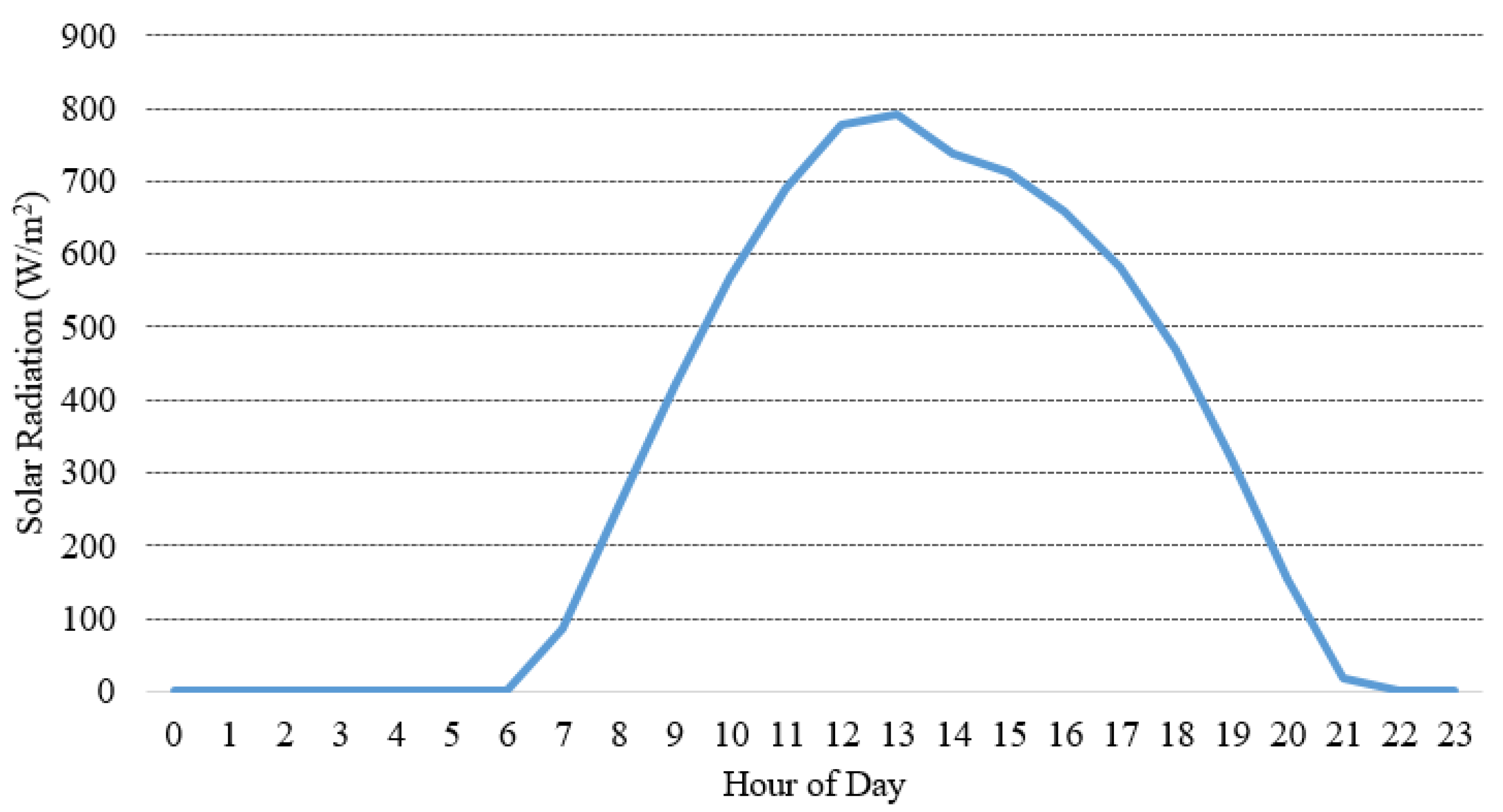
2.2. Solar Energy

Solar PV absorbs the solar radiation in a solar PV system. This absorbed sunlight dislodges electrons from the atoms of the PV cell. The passage of free electrons generates current that is transmitted via wires. Monocrystalline and polycrystalline solar cells are the two most common forms. Other forms of solar photovoltaics include organic cells, thin-film cells, and perovskites. However, both polycrystalline and monocrystalline materials are used for industrial and residential applications. There are mainly two types of solar panel configurations: 60-cell and 72-cell. The 60-cell solar panels produce between 285 W and 315 W, whereas 72-cell solar panels produce between 335 W and 375 W. A total of 18 panels of the 72-cell solar panel are needed for a 6.5 kW installation [48]. Each 72-cell solar panel is 77 inches in length and 36 inches in width. Therefore, about 5 ${\mathrm{m}}^2$ of space is needed for a 1 kW solar panel.

Solar photovoltaics (PVs) are an excellent technique to generate sustainable energy by converting solar radiation into electricity. Solar radiation data is gathered from the Meteoblue data centre [49]. The following is the equation for determining solar output:

$$P_{pv}={\mathsf{\Gamma }}_{pv}{ϝ}_{pv}\left(\frac{I{R}_t}{I{R}_{S.T.C}}\right)\left[1+\alpha (T_t-T_{S.T.C})\right]$$

(1)

where the solar array capacity rating (kW) is denoted by ${\mathsf{\Gamma }}_{pv}$, the derating factor (%) by ${ϝ}_{pv}$, the irradiance (${\mathrm{kW}/\mathrm{m}}^2$) at time t and at standard test condition ($S.T.C$) by $I{R}_t$ and $I{R}_{S.T.C}$, respectively. The temperature coefficient ($\%{/}^{\circ }\mathrm{C}$) is represented by $\alpha$, whereas the temperature (${}^{\circ }\mathrm{C}$) for current and standard test condition time is designated by $T_t$ and $T_{S.T.C}$, respectively.

Manufacturers of solar panels determine the power rating of each panel under standard test conditions (S.T.C). The solar irradiance at S.T.C is 1 ${\mathrm{kW}/\mathrm{m}}^2$, and the temperature is 25 °C. The derating factor is included in modelling the solar array in this research. This derating factor is essential as it relates to the power loss of the panel caused by wiring and age. For actual implementation, the cell temperature is more than the standard temperature (25 °C), and if the temperature impact is ignored, the simplified equation for (1) may be written as follows:

$$P_{pv}={\mathsf{\Gamma }}_{pv}{ϝ}_{pv}\left(\frac{I{R}_t}{I{R}_{S.T.C}}\right)$$

(2)

Figure 2 shows the hourly solar radiation for a particular day. For design simplicity, it is assumed that the radiation profile will be the same throughout the project’s lifetime. A generic flat plate solar array with a capacity of 1 kW is explored in this research.

Table 2. Solar PV panel specifications.

Parameter	Value
Area occupied by unit PV panel (${\mathrm{m}}^2$)	5
Capacity (kW)	1
Initial cost (USD)	640
Replacement cost (USD)	640
O&M cost (USD/year)	0
Lifetime (years)	30
Efficiency of the MPPT unit (%)	95
Nominal operating cell temperature (${}^{\circ }\mathrm{C}$)	40
PV panel reference temperature (${}^{\circ }\mathrm{C}$)	25

summarises the precise design requirements of solar panels.

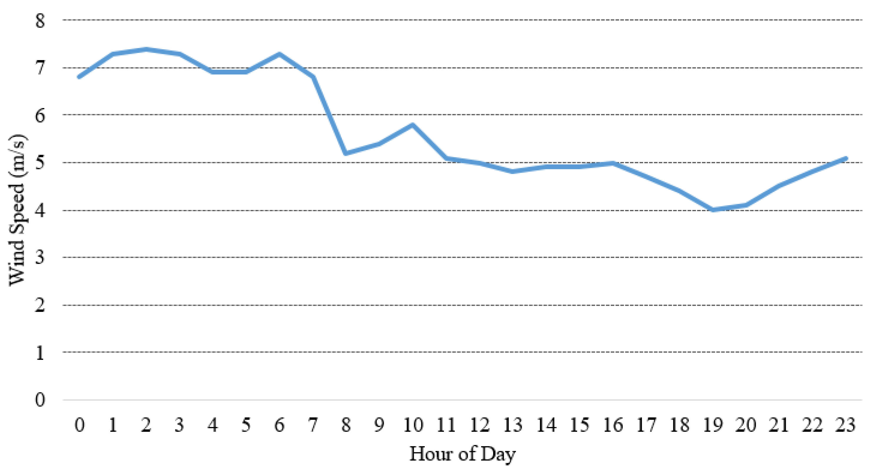
2.3. Wind Energy

A wind turbine, which uses the speed of the wind to create power, is another sustainable energy source. The output power of a wind turbine may be estimated using various models, including the Weibull parameter model [50,51], the linear model [52,53], and the quadric model. The quadric model is used in this research. Regarding the wind turbines studied in this research, the hub height is 55 m, and the hub diameter of 33 m is considered, while the nominal capacity is 10 kW. Three procedures must be completed to determine the output of a wind turbine. The first step is to determine the turbine’s hub-height wind speed. The following is the equation to determine the wind speed at hub-height [54]:

$$v_h=v_{an}\frac{H_h}{H_{an}}$$

(3)

where the wind speed (m/s) at hub height and anemometer height is represented by $v_h$ and $v_{an}$, respectively. The height (m) of the turbine hub and the anemometer is denoted by $H_h$ and $H_{an}$, respectively.

The turbine’s power at standard air density is calculated in the second step. To calculate this, a turbine power curve is needed from the manufacturers. Following the preceding step, the power may be determined at standard air density using the correct wind speed numbers. The density adjustment is the third stage. The following equation may be used to calculate the exact amount of power exerted by the turbine when employing the density correction:

$$P_{actual}=\left(\frac{\varrho }{{\varrho }_{STD}}\right)P_{STD}$$

(4)

where the turbine actual power (kW) and standard power (kW) is represented by $P_{actual}$ and $P_{STD}$, respectively. The actual air density (${\mathrm{kg}/\mathrm{m}}^3$) and standard air density (${\mathrm{kg}/\mathrm{m}}^3$) is denoted as $\varrho$ and ${\varrho }_{STD}$, respectively. Figure 3 [49] shows the wind speed profile used for this study and to reduce the computational complexity, this profile is considered for the entire project.

Table 3. Wind turbine specifications.

Parameter	Value
Capacity (kW)	10
Initial cost (USD)	13,000
Replacement cost (USD)	13,000
O&M cost (USD/year)	400
Lifetime (years)	20
Hub Height (m)	55
Rotor size (m)	33
Minimum wind speed (m/s)	4
Rated wind speed (m/s)	8
Maximum wind speed (m/s)	20

contains the wind turbine design specifications and considerations.

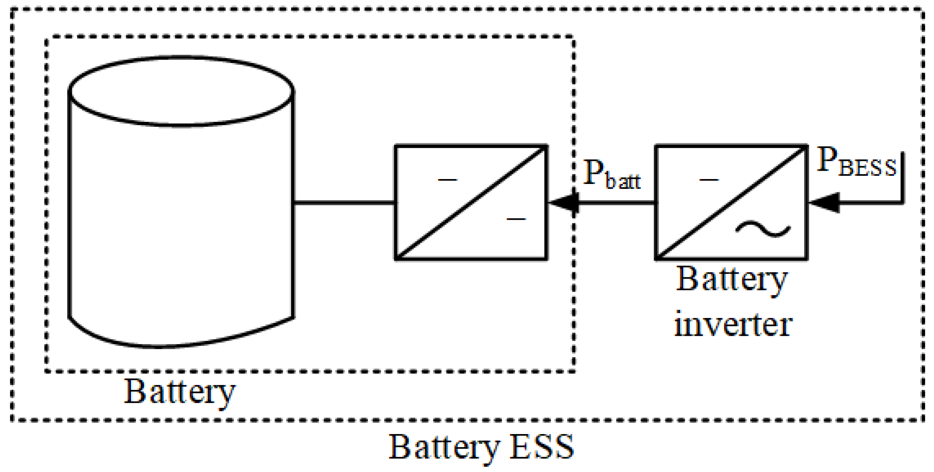
2.4. Battery Storage System

As a kind of energy storage, a 1 kWh Li-Ion battery has been analyzed in this research. This battery has a lifespan of 15 years and a capital cost of USD 180. The minimum state of charge is 20%, the maximum is 100%, and the efficiency is 90%.

The Battery Energy Storage System (BESS) coupling topology taken into account in this work is illustrated in Figure 4. The BESS is controlled by an EMS-provided reference power signal and associated control algorithms. This reference signal is compared to the $P_{rated,inv}$ and $P_{rated,batt}$, power limitations of the inverter and battery, respectively, as follows.

$$|P_{batt}|\le P_{rated,batt}$$

(5)

$$|P_{BESS}|\le P_{rated,inv}$$

(6)

Therefore, the BESS’s power output is restricted to the nominal power of the inverter. After verifying the power constraints, the battery model computes the maximum capacity based on the operating voltage range of the cell, the State of Health (SoH), and the State of Charge (SoC). The last step involves determining the system’s reaction to the power reference.

State of Charge (SoC) refers to the amount of charge remaining in a battery and is directly proportional to accessible energy. Therefore, the SoC must be calculated since it cannot be measured. The following equation is used to approximate the SoC in the MATLAB model.

$$SoC\left(k\right)=\frac{E_{batt}\left(k\right)}{E_{cap}\left(k\right)}$$

(7)

where $SoC\left(k\right)$ represents the state of charge at sample step ‘k’, $E_{batt}\left(k\right)$ represents the stored energy in the battery at sample stage ‘k’, and $E_{cap}\left(k\right)$ represents the overall capacity of the battery at sample step ‘k’. As a result of the consequences of ageing, Ecap fluctuates throughout time and diminishes continually.

Depending on whether the battery is charging or discharging, the energy stored in the battery is computed using Equation (8).

$$E_{batt}\left(k\right)=\left\{\begin{array}{cc}{E}_{batt}(k-1)+\sqrt{{\eta }_{batt}}·P_{batt}\left(k\right)·\Delta t-E_{SD},\hfill & P_{batt}\left(k\right)\ge 0\hfill \\ E_{batt}(k-1)+\frac{P_{batt}\left(k\right)·\Delta t}{\sqrt{{\eta }_{batt}}}-E_{SD},\hfill & P_{batt}\left(k\right)<0.\hfill \end{array}\right.$$

(8)

where stored energies in the battery are denoted by $E_{batt}\left(k\right)$ and $E_{batt}(k-1)$ at sample steps ‘k’ and ‘$k-1$’, respectively, the efficiency of the battery round-trip is represented by ${\eta }_{batt}$ which is assumed to be the same for charging and discharging, the battery in-out power flow is as $P_{batt}\left(k\right)$ at sample step ‘k’ (positive for charging, negative for discharging), sample time as $\Delta t$, and $E_{SD}$ is the self-discharge.

The charge limits confine the SoC within its boundaries:

$$So{C}_{min}\le SoC\le So{C}_{max}$$

(9)

2.5. Fast Charging Station

N-R HES performance was examined in this research with a fast charging station that can handle up to 1000 vehicles per day. The Alternative Fuels Data Center’s (AFDC) website was used to acquire this data. The energy consumption on a daily basis is 58,580 kWh, but it has been scaled down to 50,000 kWh, with a peak demand of 5780.80 kW and a load factor of 0.36, respectively, for research reasons; 35% charge at level I, 35% charging at level II, and 30% charging at DC high speed are all supported by this FCS. Figure 5 [55] shows the expected hourly load of the fast charging station.

3. Design of Energy Management System

The objective of this work is to establish energy management techniques to assess the efficiency of the proposed N-R HES fast charging station. Section 3.1 constructs a Model Reference Adaptive Control (MRAC). The objective function necessary for making the control strategy is described in Section 3.2, while the constraints are presented in Section 3.3. In order to define the global optimization problem, constraints and a multi-objective cost function are specified. The implementation of the suggested algorithm in the fast charging station is described in Section 3.4.

3.1. Control System Design

This section describes the design of the adaptive model reference controller. The control technique of the developed controller is shown in Figure 6. Based on adjustable controller variables, the model-reference adaptive control technique is designed. Adjustments are made to the controller’s parameters in order for the ideal plant to follow the reference model.

The proposed controller consists of a reference model, a controller, and an adaptive mechanism. Reference models are selected based on their ability to reproduce the desired response. The controller was made up of a number of adjusting parameters that could be adjusted individually. The control rule is explained in this study using the parameter $\theta$, which is related to the adaptation gain. The results of the comparison between the reference model and the plant model are sent to the adaptive mechanism via the controller.

Applying this reference model’s control parameter is one of the goals of the adaptive mechanism. A variety of strategies, such as Lyapunov theory and augmented error theory, MIT rule, etc., are often used to broaden the scope of the adaptive mechanism. The MIT law is altered in this study in order to increase the adaptive mechanism. It is seen in Figure 6 that tracking error is expressed by “e” in terms of the difference between the $Y_{model}$ and $Y_{plant}$ models.

$$\begin{array}{c}\hfill e=Y_{plant}-Y_{model}\end{array}$$

(10)

Using a closed-loop system for unknown parameters, the proposed controller is able to modify the plant response to the reference model. Equation (10) is used to derive a cost function. According to the following formula, where J is a cost function of $\theta$ may be deduced:

$$\begin{array}{c}\hfill J\left(\theta \right)=\frac{e^2\left(\theta \right)}{2}\end{array}$$

(11)

where the adjustable parameter is represented by $\theta$. The parameter is modified in order to reduce the cost function to zero. To do this, the change in the parameter ($\theta$) is assumed to be proportional to the negative gradient of J.

$$\begin{array}{c}\hfill \frac{d\theta }{dt}=-\gamma \frac{\delta J}{\delta \theta }=-\gamma e\frac{\delta e}{\delta \theta }\end{array}$$

(12)

where the sensitivity derivative is defined by the differential coefficient term $\frac{\delta e}{\delta \theta }$. The MIT rule describes the relation between the change in $\theta$ and the cost function J. Here, a positive number of $\gamma$ might determine the controller’s adjustable gain.

$$\begin{array}{c}\hfill J\left(\theta \right)=\left|e\right(\theta \left)\right|\end{array}$$

(13)

$$\begin{array}{c}\hfill \frac{d\theta }{dt}=-\gamma e\frac{\delta e}{\delta \theta }sign\left(e\right)\end{array}$$

(14)

where

$$sign\left(e\right)=\left\{\begin{array}{c}\hfill -1,e<0\hfill \\ \hfill 0,e=0\hfill \\ \hfill 1,e>0\hfill \end{array}\right.$$

Assume the approach is linear with the transfer function KG(s), where K is an unknown parameter, and G(s) is a known transfer function of the 2nd order. The objective is to develop a controller that will allow the proposed technique to monitor the reference model with the transfer function $\frac{Y\left(s\right)}{U\left(s\right)}=K_{0}G\left(s\right)$, where $k_0$ is a known parameter. From (10), we derive

$$\begin{array}{c}\hfill e=Y_{plant}-Y_{model}\\ \hfill =kG\theta U-k_{0}GU\end{array}$$

(15)

Now, the update rule is,

$$\frac{\delta e}{\delta \theta }=kGU=\frac{k}{k_0}{Y}_{model}$$

(16)

From (14), it can be written as

$$\frac{d\theta }{dt}=-{\gamma }^{\prime }\frac{k}{k_0}{Y}_{model}e=-\gamma Y_{model}e$$

(17)

This is referred to as the update MIT rule, and it is used to develop the legislation for adjusting parameter $\theta$. In this study, the given approach is applied to a second-order MIT law system.

Equation (17) evaluates adaptation gain ($\gamma$), an additional essential term for an adaptive system. For optimal tracking performance, the adaption gain is set at 0.001 for the system’s high tracking performance.

3.2. Objective Function

To optimize operation, the optimization issue must include formulating an objective function. This thesis examines a single-objective optimization problem that aims to obtain an optimum solution for many competing objectives. This paper addresses an N-R HES planning issue with a single aim to reduce generating costs. In formulating the optimization issue, technical and economic elements are consolidated. It is important to develop an optimization fitness function to acquire the best system design with the lowest energy cost. The fitness function is the total energy costs of every system component. The objective function may be defined as follows for the minimization problem.

$${}_{min}{f}_R={\mathsf{\Sigma }}_{iϵk}{R}_i$$

(18)

where k is the set of system components and $R_i$ is the energy generation cost of the Rth component. Components of the system include MMR, solar PV, wind turbine, and ESS. The cost of energy production of any element indicates the present value of the component’s entire cost, which includes the cost of fuel, fuel consumption, total operating cost, O&M cost, and start-up cost. Any system component’s cost function may be represented as follows:

$$\begin{array}{c}\hfill \sum _{t=1}^{t=24}{R}_{t,HES}=C_{HES}{F}_{HES}{\mathrm{\Sigma }}_{t=1}^{t=24}{P}_{t,HES}\Delta t\hfill \\ \hfill +{\mathrm{\Sigma }}_{t=1}^{t=24}O{M}_{t,HES}+{\mathrm{\Sigma }}_{t=1}^{t=24}S{C}_{t,HES}\end{array}$$

(19)

where $R_{t,HES}$ is the total operating cost hybrid energy system, $C_{HES}$ is the fuel cost of the HES unit ($USD/m^3$), $F_{HES}$ is the fuel consumption rate ($m^3/kWh$), $P_{t,HES}$ is the power output from the HES, $O{M}_{t,HES}$ is the operation and maintenance cost, $S{C}_{t,HES}$ is the start-up cost, and $\Delta t$ is the time step.

The aim is to effectively use the HES such that the total generation cost is minimized. It can be conducted by storing the excess energy to the ESS and utilize them during the pick hour and also selling them to the utility; hence, the cost of energy is reduced. The following equation can be used as an expression:

$$R=\sum _{k=0}^{N-1}(W_{buy}\left(k\right)·P_{buy}\left(k\right)-W_{sell}\left(k\right)·P_{sell}\left(k\right))\Delta t$$

(20)

where step horizon of the optimization is denoted by N, the buying energy from the hybrid energy system at time ‘k’ is represented by $W_{buy}\left(k\right)$, whereas $W_{sell}\left(k\right)$ is the selling price of the energy generated by the system. $P_{sell}\left(k\right)$ and $P_{buy}\left(k\right)$ represents the to and from power flow of the system, respectively, and $\Delta t$ is the sample time.

The energy bill will be reduced if the cost function is minimized. Nonetheless, repeated cycling of the ESS will diminish its lifespan. Therefore, each charge or discharge cycle incurs a cost, and it is preferable to decrease the number of cycles each day. The optimization problem should thus include, in addition to the overall HES cost function, a cost function reflecting the opportunity costs of ESS cycles. The opportunity costs of ESS cycles may be computed using the Formula (21), where the change in storage energy ($\Delta E_{ESS}$), is multiplied by an ESS cost weight ($c_b$) in order to penalize energy storage cycles.

$$R_{ESS}={\mathrm{\Sigma }}_{k=0}^{N-1}\Delta E_{ESS}\left(k\right)·c_b$$

(21)

where $\Delta E_{ESS}\left(k\right)$ represents the absolute change in storage energy between time steps k and $k-1$. The following equation calculates $\Delta E_{ESS}\left(k\right)$:

$$\begin{array}{ccc}\hfill \Delta E_{ESS}\left(k\right)& =& \hfill |E_{ESS}\left(k\right)-E_{ESS}(k-1)|\hfill \\ & =& \hfill \left({\eta }_{ch}·P_{ch}\left(k\right)+\frac{P_{dis}\left(k\right)}{{\eta }_{dis}}\right)·\Delta t\hfill \end{array}$$

(22)

The final expression of the energy storage cost function can be achieved by combining Equations (21) and (22) and is as follows:

$$R_{ESS}={\mathrm{\Sigma }}_{k=0}^{N-1}\left({\eta }_{ch}·P_{ch}\left(k\right)+\frac{P_{dis}\left(k\right)}{{\eta }_{dis}}\right)·\Delta t·c_b$$

(23)

The ESS cost function lowers storage degradation by executing only those actions that provide more profitability than cycle opportunity costs. In this manner, ESS degradation is included in the optimization model.

3.3. Constraints

The optimization problem uses constraints to assure the dependability, resilience and enhanced performance of the proposed energy systems. Some restrictions are utilized to handle various real-world limits to construct the energy systems in the fast charging station. Any energy source’s output must be equal to or less than its maximum capacity. This may be shown as follows:

$$P_{gen}^j\left(t\right)\le P_{gen,max}^j$$

(24)

where $P_{gen}^j\left(t\right)$ is the power generation and $P_{gen,max}^j$ is the maximum power generation of the jth component at time step t.

To guarantee the system’s stability and resilience, the total system generation must be higher than or equal to the entire system demand. The following equations are used to express the system’s energy management constraints.

$$\sum P_{gen}^j\left(t\right)\ge \sum _{t=1}^{t_{total}}{P}_{EL}^j\left(t\right)$$

(25)

$$\begin{array}{c}\hfill \sum P_{gen}^j\left(t\right)=\sum _{t=1}^{t_{total}}Nu{m}_{PV}{P}_{PV}\left(t\right)+\sum _{t=1}^{t_{total}}Nu{m}_{WT}{P}_{WT}\left(t\right)\hfill \\ \hfill +\sum _{t=1}^{t_{total}}Nu{m}_{MMR}{P}_{MMR}\left(t\right)\end{array}$$

(26)

where $P_{gen}^j\left(t\right)$ refers to the power generation, $P_{EL}^j\left(t\right)$ to the power demand at time t of the year j. $Nu{m}_{PV}$, $Nu{m}_{WT}$, and $Nu{m}_{MMR}$ indicate the number of solar PV, wind turbine, and MMR, respectively. $P_{PV}$, $P_{WT}$, and $P_{MMR}$ refer to the power produced by the solar PV, wind turbine, and MMR at the time t, sequentially.

This energy storage device is used to store extra energy. This research takes into account the following constraints to provide adequate energy management of the system and maintain the required SoC of the storage device.

$$SoC\left(k\right)=\left\{\begin{array}{cc}\hfill \frac{P_{ESS}\left(k\right)}{{\eta }_{dis}·E_{cap}\left(k\right)}·\Delta t+SoC(k-1),\hfill & \hfill P_{ESS}\left(k\right)<0\hfill \\ \hfill \frac{{\eta }_{ch}·P_{ESS}\left(k\right)}{E_{cap}\left(k\right)}·\Delta t+SoC(k-1),\hfill & \hfill P_{ESS}\left(k\right)\ge 0\hfill \end{array}\right.$$

(27)

where $\frac{P_{ESS}\left(k\right)}{E_{cap}\left(k\right)}$ denotes the change in storage energy at time interval $\Delta t$, ${\eta }_{dis}$ and ${\eta }_{ch}$ represents the efficiency of the storage system during discharging and charging. The total storage capacity at any time ‘k’ is expressed by $E_{cap}\left(k\right)$ which is not constant rather decreases gradually over the time due to aging effects. The state of charge during time ‘k’ and ‘$k-1$’ is given by $SoC\left(k\right)$ and $SoC(k-1)$, respectively.

If $P_{ESS}$ is positive, the energy storage system is charging, and if it is negative, it is discharging. To express this logical state and prevent simultaneous charging and discharging of the storage system, a binary variable with the value of (28) is included in the model.

$${\delta }_b\left(k\right)=\left\{\begin{array}{cc}\hfill 0,\hfill & \hfill \mathrm{for} \mathrm{charging}\hfill \\ \hfill 1,\hfill & \hfill \mathrm{for} \mathrm{discharging}.\hfill \end{array}\right.$$

(28)

Finally, SoC of the ESS can be described by one equation by combining the properties of charging and discharging as follows:

$$SoC\left(k\right)=\frac{{\eta }_{ch}·P_{ch}\left(k\right)}{E_{cap}\left(k\right)}·\Delta t-\frac{P_{dis}\left(k\right)}{{\eta }_{dis}·E_{cap}\left(k\right)}·\Delta t+SoC(k-1)$$

(29)

Limiting the SoC range will enhance the storage lifespan by preventing deep discharging and overcharging. The constraint below indicates the minimum and maximum SoC limits:

$$So{C}_{min}\le SoC\left(k\right)\le So{C}_{max}$$

(30)

Finally, the overall SoC constraint can be achieved by combining Equations (29) and (30).

$$\begin{array}{c}\hfill So{C}_{min}-SoC(k-1)\le \frac{{\eta }_{ch}·P_{ch}\left(k\right)}{E_{cap}\left(k\right)}·\Delta t-\frac{P_{dis}\left(k\right)}{{\eta }_{dis}·E_{cap}\left(k\right)}·\Delta t\hfill \\ \hfill \le So{C}_{max}-SoC(k-1)\end{array}$$

(31)

Last but not least, constraints on the storage power are imposed to represent the maximum power that may be charged/discharged by the storage system during a predetermined time period. The ESS power restrictions for discharging and charging may be described using Equation (28) as follows:

$${\delta }_b\left(k\right)P_{dis}^{min}\le P_{dis}\left(k\right)\le {\delta }_b\left(k\right)P_{dis}^{max}$$

(32)

$$(1-{\delta }_b\left(k\right))P_{ch}^{min}\le P_{ch}\left(k\right)\le (1-{\delta }_b\left(k\right))P_{ch}^{max}$$

(33)

The fast charging station must always maintain a balance between its power generation and consumption. This is achieved by constantly meeting the requirements of Equation (34), which include power conversion efficiency and positive power directions.

$$\begin{array}{c}\hfill P_{load}\left(k\right)=P_{PV}\left(k\right)+P_{WT}\left(k\right)+P_{MMR}\left(k\right)+{\eta }_{inv}\left(k\right)·P_{dis}\left(k\right)\hfill \\ \hfill -\frac{P_{ch}\left(k\right)}{{\eta }_{inv}\left(k\right)}+P_{buy}\left(k\right)-P_{sell}\left(k\right)\end{array}$$

(34)

where $P_{load}\left(k\right)$, $P_{PV}\left(k\right)$, $P_{WT}\left(k\right)$, and $P_{MMR}\left(k\right)$ are the forecasted load demand, PV output power, wind output power, and MMR output power, respectively. The storage system inverter efficiency (${\eta }_{inv}\left(k\right)$) varies depending on the storage power.

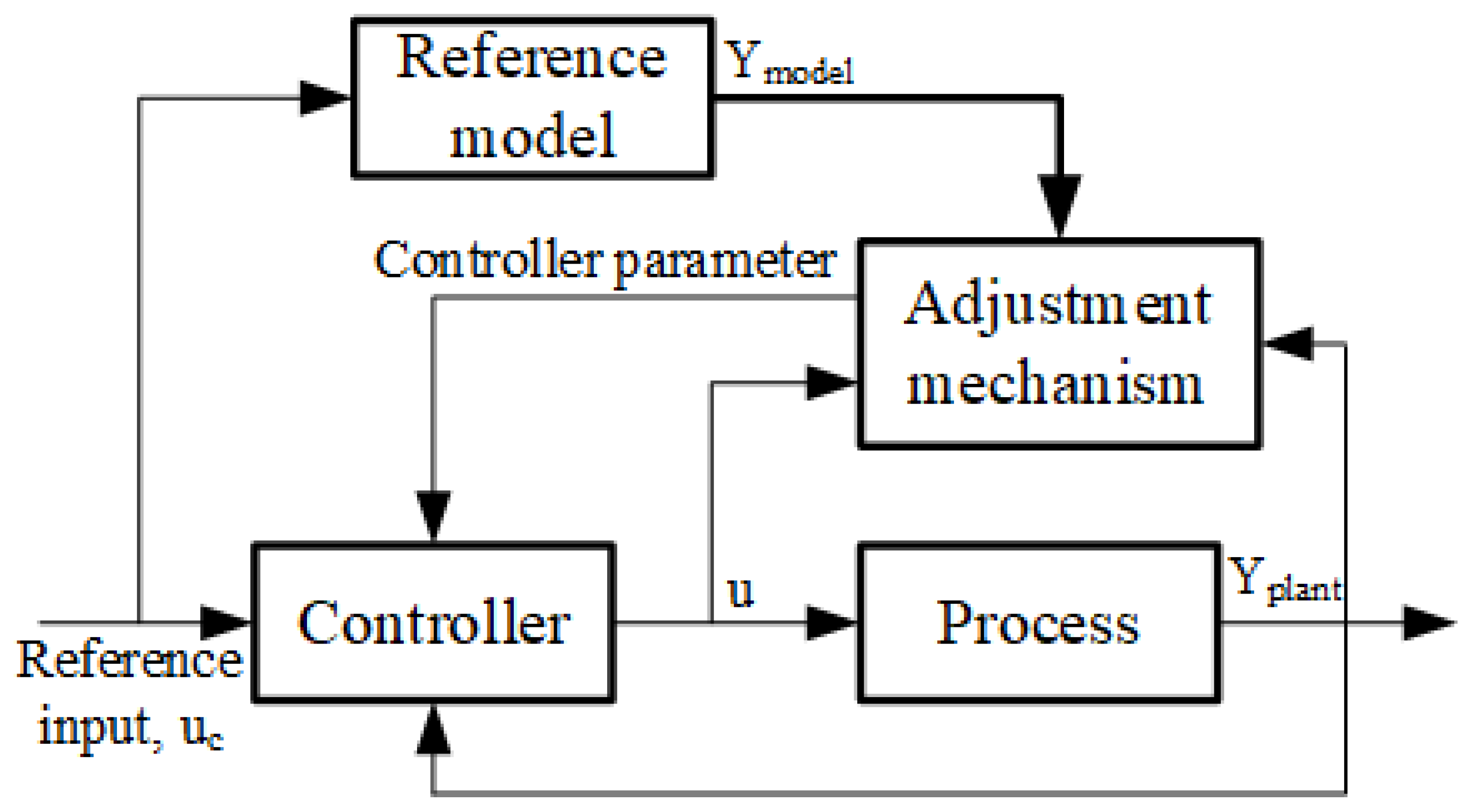
3.4. Mrac with Mixed-Integer Linear Programming

The entire optimization issue may be stated as follows, taking into account the constraints and objective function established in the preceding sections:

$$\begin{array}{cc}\hfill \mathrm{l}\mathrm{l}\mathrm{m}\mathrm{i}\mathrm{n}\mathrm{i}\mathrm{m}\mathrm{i}\mathrm{z}\mathrm{e}& \mathrm{R} \left(18\right)\hfill \\ \hfill \mathrm{s}\mathrm{u}\mathrm{b}\mathrm{j}\mathrm{e}\mathrm{c}\mathrm{t} \mathrm{t}\mathrm{o}& \mathrm{b}\mathrm{i}\mathrm{n}\mathrm{a}\mathrm{r}\mathrm{y} \mathrm{v}\mathrm{a}\mathrm{r}\mathrm{i}\mathrm{a}\mathrm{b}\mathrm{l}\mathrm{e}\mathrm{s} \left(28\right)\hfill \\ \hfill & \mathrm{s}\mathrm{t}\mathrm{o}\mathrm{r}\mathrm{a}\mathrm{g}\mathrm{e} \mathrm{m}\mathrm{o}\mathrm{d}\mathrm{e}\mathrm{l} \left(29\right)\hfill \\ \hfill & \mathrm{s}\mathrm{t}\mathrm{o}\mathrm{r}\mathrm{a}\mathrm{g}\mathrm{e} \mathrm{c}\mathrm{o}\mathrm{n}\mathrm{s}\mathrm{t}\mathrm{r}\mathrm{a}\mathrm{i}\mathrm{n}\mathrm{t}\mathrm{s} \left(31\right)\hfill \\ \hfill & \mathrm{p}\mathrm{o}\mathrm{w}\mathrm{e}\mathrm{r} \mathrm{b}\mathrm{a}\mathrm{l}\mathrm{a}\mathrm{n}\mathrm{c}\mathrm{e} \left(34\right)\hfill \end{array}$$

(35)

Due to the nonlinear dynamics of the ESS capacity and power electronic efficiency, this issue is defined as a Mixed-Integer Nonlinear Programming (MINLP) problem with a non-convex cost function. When this MINLP optimization issue is resolved, the optimum schedule is generated. However, this schedule will be uncertain; the system model will be flawed, there will be forecasting errors, and the system state will not develop as projected. The open-loop solution to the single optimization issue does not account for these uncertainties.

A Model Reference Adaptive Control (MRAC) framework may be used alternatively to tackle the optimization issue. Thus, a method for feedback control is established, which may compensate for the uncertainties. In addition, the MRAC method allows the power converter efficiency and ESS capacity to be estimated and updated prior to each optimization sample and then assumed constant along the forecast horizon. In this manner, the optimization problem is converted into a MILP problem, which is preferred over the corresponding MINLP formulation due to, for example, a guaranteed optimal solution, access to available solvers, and less computational effort with no discernible loss of accuracy compared to MINLP.

This research presents a control strategy that combines MRAC and MILP to account for uncertainties effectively and to capture a portion of the system’s nonlinear dynamics by updating the system model at each time step. This section describes the MRAC strategy designed for energy management in fast charging stations. Figure 7 displays a block diagram of the MRAC system with MILP, and the following paragraphs discuss the four phases that define the approach used by the control strategy.

Steps associated with the implementing of MRAC with MILP are discussed in detail as follows.

3.4.1. Optimization Problem Formulation

Based on the most recent updates to the system states and power electronic efficiency values, as well as predictions for future PV, WT, and MMR output levels, load requirements, and energy costs, an optimization problem has been developed for a chosen prediction horizon ($N_p$). The previous system unit model is used to update the present system states. In addition, the formula stated by (36) [56] is used to update the efficiency of power electronics.

$${\eta }_{inv}=\frac{p}{p+p_0+k{p}^2}$$

(36)

where for a high efficiency inverter, $p=\frac{|p_{o}ut|}{p_{rated,inv}}$ with $p_0=0.007$ and $k=0.045$.

A forecasting module may be implemented in the proposed MRAC-based EMS, as shown in Figure 7, and it will be able to estimate the load demand, PV, WT and MMR production, as well as energy prices, at each time step of the given prediction horizon, $k=1,...,N_p$. The entire optimization problem presented in Equation (35) must be rewritten into a form that can be addressed using an accessible MILP solver in order to be solved. Since the $intlinprog$ solver in MATLAB will be used in this thesis, the optimization problem must be restated in the matrix form provided by (37).

$$\begin{array}{cc}\hfill \mathrm{m}\mathrm{i}\mathrm{n}\mathrm{i}\mathrm{m}\mathrm{i}\mathrm{z}\mathrm{e} \mathrm{u}& R^{T}u\hfill \\ \hfill \mathrm{s}\mathrm{u}\mathrm{b}\mathrm{j}\mathrm{e}\mathrm{c}\mathrm{t} \mathrm{t}\mathrm{o}& u\left(intcon\right) \mathrm{a}\mathrm{r}\mathrm{e} \mathrm{i}\mathrm{n}\mathrm{t}\mathrm{e}\mathrm{g}\mathrm{e}\mathrm{r}\mathrm{s}\hfill \\ \hfill & A_{ineq}·u\le b_{ineq}\hfill \\ \hfill & A_{eq}·u=b_{eq}\hfill \\ \hfill & lb\le u\le ub\hfill \end{array}$$

(37)

where

• the vector $u\left(k\right)=\begin{array}{ccccc}[P_{ch}\left(k\right)& P_{dis}\left(k\right)& {\delta }_b\left(k\right)& P_{buy}\left(k\right)& P_{sell}\left(k\right)]\end{array}$ is used to collect the decision variables for $k=0,...,N_p-1$;
• the integer constraints are represented as a vector called $intcon$, and the integer-valued components of decision vector u are indicated by the $intcon$ values;
• a vector form with linear coefficients is used to define the objective function R (18);
• $ub$ and $lb$ denote the lower limit and upper limit of the decision variable (28);
• Matrix $A_{ineq}$, vector $b_{ineq}$, and decision vector u are used to define the inequality constraint (29);
• Matrix $A_{eq}$, vector $b_{eq}$, and decision vector u are used to represent the equality constraint (34).

3.4.2. Optimization Problem Solution

In (37), the optimum input sequence for the prediction horizon $N_p$ is found by solving the MILP problem.

$$u_{opt}\left(k\right)=\left[\begin{array}{cccc}{\left(u_{opt}\left(0\right)\right)}^T& {\left(u_{opt}\left(1\right)\right)}^T& \dots & {\left(u_{opt}(N_p-1)\right)}^T\end{array}\right]$$

(38)

where each vector is the future optimal input sequence for the sample time $k=0,1,\dots ,N_p-1$, respectively.

3.4.3. Control Set-Points Execution

Although a whole series of $N_p$ future control signals is calculated, only $u_{opt}\left(0\right)$ is applied to the system, and the other optimum values in $u_{opt}\left(k\right)$ are omitted.

3.4.4. Shift the Prediction Horizon

The prediction horizon is shifted, and steps 3.4.1–3.4.3 are repeated to generate a new optimum sequence, $u_{opt}\left(k\right)$. All this is conducted by re-evaluating the system’s current state, re-calculating power electronic efficiencies, and then resolving a new optimization issue. In this receding horizon technique, there is a feedback mechanism where the new optimum plan might possibly adjust for any disturbances that have occurred in the system since the previous one.

4. Performance Evaluation

This section details the performance of the MILP-MRAC algorithm. The implementation of the suggested energy management system in conducted in MATLAB simulink environment. Initially, the MILP optimization technique is expressed as a MATLAB function using the MILP solver $intlinprog$. A discrete update technique is chosen for the MATLAB function block, meaning that the block is sampled at the rate provided by its sample time attribute. Thus, the optimization is re-executed at each sample interval, and a feedback system (MRAC) is established.

Note that the $intlinprog$ function is not supported by the MATLAB function block’s code generator. In order to resolve this issue, the optimization function must be marked as intrinsic inside the code generating script. The block’s initialization script initializes all inputs to the MATLAB Function block, and the block’s inputs are as follows:

• SoC values estimated from the energy storage block;
• The step horizon of forecasting;
• MILP’s sampling rate, or the number of times it calls itself in Simulink;
• Predicted statistics on the cost of electricity produced by a forecasting function for PV, WT, and MMR generation and the demand for electricity;
• the nominal storage capacity;
• efficiency of the power electronics which is updated at each time step.

The performance of the hybrid energy system is then investigated. Figure 8 shows the performance of the proposed HES with the inclusion of a conventional energy management system (meta-heuristic). In this figure, it can be seen that the combined energy production by the N-R HES can fulfill the power demand of the fast charging station but it generates more excess energy after meeting the load demand and the storage capacity of the ESS. This excess energy is a waste and at the same time it increases the generation cost of the energy. To overcome this problem, the proposed energy management system has been included to the system and the performance is presented in Figure 9. In this figure, it can be seen that the proposed EMS system can predict efficiently the load demand with the help of the forecast function and thus enables the system to produce required amount of energy to meet the load demand and the ESS capacity. In this way, energy waste problem has been solved. Figure 10 justifies this claim where it shows that around 22% of energy wastage has been reduced by the proposed EMS system.

By comparing this two scenarios, operation variation of ESS can also be seen. The adaptive mechanism helps the EMS system to schedule the operation of the energy storage system in an optimized way such that the storage system is charged while the power generation can meet the load demand and the storage SoC is less than 50%. Then the storage system will be charged until it reaches to its limit and as soon as it reaches to 80% of its SoC, the charging controller will disconnect the ESS from being charged furthermore. The control strategy regulates the operation time of the ESS with the help of forecast function and cost function. When the energy generation from the RESs is limited due to their availability and the cost of energy is high, then the EMS system will check the storage SoC status and if that satisfies the condition, the controller will connect the ESS to the HES again and enables it to discharge. The SoC status of the ESS during this operation is shown in Figure 11. ESS performance has been examined with inclusion of both the conventional and proposed energy management system. This figure indicates that the proposed system optimizes the ESS operation and thus improves the overall system performance.

Figure 12 shows the cost of energy for both case scenarios. From this figure, it can be seen that the cost of energy production is higher for the conventional system ranging from $USD0.19/\mathrm{kWh}$ to $USD0.31/\mathrm{kWh}$. This has been reduced with the inclusion of the proposed EMS system. For the proposed system the cost of energy ranges from $USD0.17/\mathrm{kWh}$ to $USD0.26/\mathrm{kWh}$ which is 16% lower than the base system and hence, justifies the effectiveness of the proposed system.

5. Conclusions

In conclusion, this study offers a simplified architecture of a nuclear–renewable hybrid energy system to support a fast charging station for the electrification of transportation. This research also focused on the development of an energy management system for a grid-isolated nuclear–renewable hybrid energy system. Overall, the objective was to design a control approach that combines mixed-integer linear programming with a model reference adaptive control to effectively account for uncertainties and capture part of the nonlinear dynamics of the system by updating the system model at each time step. Finally, mathematical modelling has been built in MATLAB and optimized using a mixed-integer linear programming approach and model reference adaptive control strategy for the system’s energy management. The performance of the suggested optimization strategy is determined by comparing the cost of energy, power savings, and storage usage. From the performance analysis, it can be seen that the proposed method can effectively manage the power usage from the hybrid energy system while reducing the power loss and the cost of energy. The future work of this study can be extended to analyze the grid integration in the optimization, consider demand-side management strategy, and experimental verification.

References

- Barone, G.; Buonomano, A.; Calise, F.; Forzano, C.; Palombo, A. Building to vehicle to building concept toward a novel zero energy paradigm: Modelling and case studies. Renew. Sustain. Energy Rev. 2019, 101, 625–648. [Google Scholar] [CrossRef]
- Sujitha, N.; Krithiga, S. RES based EV battery charging system: A review. Renew. Sustain. Energy Rev. 2017, 75, 978–988. [Google Scholar] [CrossRef]
- Hansen, K.; Mathiesen, B.V.; Skov, I.R. Full energy system transition towards 100% renewable energy in Germany in 2050. Renew. Sustain. Energy Rev. 2019, 102, 1–13. [Google Scholar] [CrossRef]
- Rhys-Tyler, G.; Legassick, W.; Bell, M. The significance of vehicle emissions standards for levels of exhaust pollution from light vehicles in an urban area. Atmos. Environ. 2011, 45, 3286–3293. [Google Scholar] [CrossRef]
- Medora, N.K. Electric and Plug-in Hybrid Electric Vehicles and Smart Grids. In The Power Grid; Elsevier: Amsterdam, The Netherlands, 2017; pp. 197–231. [Google Scholar]
- Tan, Z.; Tan, Q.; Rong, M. Analysis on the financing status of PV industry in China and the ways of improvement. Renew. Sustain. Energy Rev. 2018, 93, 409–420. [Google Scholar] [CrossRef]
- Chen, W.; Hong, J.; Yuan, X.; Liu, J. Environmental impact assessment of monocrystalline silicon solar photovoltaic cell production: A case study in China. J. Clean. Prod. 2016, 112, 1025–1032. [Google Scholar] [CrossRef]
- Lee, H.; Lovellette, G. Will Electric Cars Transform the US Vehicle Market. An Analysis of the Key Determinants; Belfer Center for Science and International Affairs: Cambridge, MA, USA, 2011. [Google Scholar]
- Xu, Z.; Hu, Z.; Song, Y.; Luo, Z.; Zhan, K.; Wu, J. Coordinated charging strategy for PEVs charging stations. In Proceedings of the 2012 IEEE Power and eNergy Society General Meeting, San Diego, CA, USA, 22–26 July 2012; pp. 1–8. [Google Scholar]
- Cao, Y.; Tang, S.; Li, C.; Zhang, P.; Tan, Y.; Zhang, Z.; Li, J. An optimized EV charging model considering TOU price and SOC curve. IEEE Trans. Smart Grid 2011, 3, 388–393. [Google Scholar] [CrossRef]
- Fazelpour, F.; Vafaeipour, M.; Rahbari, O.; Rosen, M.A. Intelligent optimization to integrate a plug-in hybrid electric vehicle smart parking lot with renewable energy resources and enhance grid characteristics. Energy Convers. Manag. 2014, 77, 250–261. [Google Scholar] [CrossRef]
- Vermaak, H.J.; Kusakana, K. Design of a photovoltaic–wind charging station for small electric Tuk–tuk in DR Congo. Renew. Energy 2014, 67, 40–45. [Google Scholar] [CrossRef]
- Hafez, O.; Bhattacharya, K. Optimal design of electric vehicle charging stations considering various energy resources. Renew. Energy 2017, 107, 576–589. [Google Scholar] [CrossRef]
- Fathabadi, H. Novel wind powered electric vehicle charging station with vehicle-to-grid (V2G) connection capability. Energy Convers. Manag. 2017, 136, 229–239. [Google Scholar] [CrossRef]
- Tushar, M.H.K.; Assi, C.; Maier, M.; Uddin, M.F. Smart microgrids: Optimal joint scheduling for electric vehicles and home appliances. IEEE Trans. Smart Grid 2014, 5, 239–250. [Google Scholar] [CrossRef]
- Hutson, C.; Venayagamoorthy, G.K.; Corzine, K.A. Intelligent scheduling of hybrid and electric vehicle storage capacity in a parking lot for profit maximization in grid power transactions. In Proceedings of the 2008 IEEE Energy 2030 Conference, Atlanta, GA, USA, 17–18 November 2008; pp. 1–8. [Google Scholar]
- Acha, S.; Green, T.C.; Shah, N. Effects of optimised plug-in hybrid vehicle charging strategies on electric distribution network losses. In Proceedings of the IEEE PES T&D 2010, New Orleans, LA, USA, 19–22 April 2010; pp. 1–6. [Google Scholar]
- Vaya, M.G.; Andersson, G. Centralized and decentralized approaches to smart charging of plug-in vehicles. In Proceedings of the 2012 IEEE Power and Energy Society General Meeting, San Diego, CA, USA, 22–26 July 2012; pp. 1–8. [Google Scholar]
- Torreglosa, J.P.; García-Trivi no, P.; Fernández-Ramirez, L.M.; Jurado, F. Decentralized energy management strategy based on predictive controllers for a medium voltage direct current photovoltaic electric vehicle charging station. Energy Convers. Manag. 2016, 108, 1–13. [Google Scholar] [CrossRef]
- García-Trivi no, P.; Torreglosa, J.P.; Fernández-Ramírez, L.M.; Jurado, F. Control and operation of power sources in a medium-voltage direct-current microgrid for an electric vehicle fast charging station with a photovoltaic and a battery energy storage system. Energy 2016, 115, 38–48. [Google Scholar] [CrossRef]
- González-Rivera, E.; Sarrias-Mena, R.; García-Trivi no, P.; Fernández-Ramírez, L.M. Predictive energy management for a wind turbine with hybrid energy storage system. Int. J. Energy Res. 2020, 44, 2316–2331. [Google Scholar] [CrossRef]
- Song, Y.; Zheng, Y.; Hill, D.J. Optimal scheduling for EV charging stations in distribution networks: A convexified model. IEEE Trans. Power Syst. 2016, 32, 1574–1575. [Google Scholar] [CrossRef]
- Zheng, H.; Wu, J.; Wu, W.; Wang, Y. Integrated motion and powertrain predictive control of intelligent fuel cell/battery hybrid vehicles. IEEE Trans. Ind. Informatics 2019, 16, 3397–3406. [Google Scholar] [CrossRef]
- Hu, J.; Shan, Y.; Guerrero, J.M.; Ioinovici, A.; Chan, K.W.; Rodriguez, J. Model predictive control of microgrids–An overview. Renew. Sustain. Energy Rev. 2021, 136, 110422. [Google Scholar] [CrossRef]
- Rodriguez, J.; Heydari, R.; Rafiee, Z.; Young, H.A.; Flores-Bahamonde, F.; Shahparasti, M. Model-free predictive current control of a voltage source inverter. IEEE Access 2020, 8, 211104–211114. [Google Scholar] [CrossRef]
- Chen, T.; Abdel-Rahim, O.; Peng, F.; Wang, H. An Improved Finite Control Set-MPC-Based Power Sharing Control Strategy for Islanded AC Microgrids. IEEE Access 2020, 8, 52676–52686. [Google Scholar] [CrossRef]
- Jayachandran, M.; Ravi, G. Predictive power management strategy for PV/battery hybrid unit based islanded AC microgrid. Int. J. Electr. Power Energy Syst. 2019, 110, 487–496. [Google Scholar] [CrossRef]
- Abdeltawab, H.H.; Mohamed, Y.A.R.I. Market-oriented energy management of a hybrid wind-battery energy storage system via model predictive control with constraint optimizer. IEEE Trans. Ind. Electron. 2015, 62, 6658–6670. [Google Scholar] [CrossRef]
- e Silva, D.P.; Salles, J.L.F.; Fardin, J.F.; Pereira, M.M.R. Management of an island and grid-connected microgrid using hybrid economic model predictive control with weather data. Appl. Energy 2020, 278, 115581. [Google Scholar] [CrossRef]
- Nair, U.R.; Costa-Castelló, R. A model predictive control-based energy management scheme for hybrid storage system in islanded microgrids. IEEE Access 2020, 8, 97809–97822. [Google Scholar] [CrossRef]
- Žilinskas, A. Practical Mathematical Optimization: An Introduction to Basic Optimization Theory and Classical and New Gradient-Based Algorithms; INFORMS: Houston, TX, USA, 2006. [Google Scholar]
- Zhao, Y.; Lu, Y.; Yan, C.; Wang, S. MPC-based optimal scheduling of grid-connected low energy buildings with thermal energy storages. Energy Build. 2015, 86, 415–426. [Google Scholar] [CrossRef]
- Parisio, A.; Rikos, E.; Glielmo, L. A model predictive control approach to microgrid operation optimization. IEEE Trans. Control. Syst. Technol. 2014, 22, 1813–1827. [Google Scholar] [CrossRef]
- Jiang, Q.; Xue, M.; Geng, G. Energy management of microgrid in grid-connected and stand-alone modes. IEEE Trans. Power Syst. 2013, 28, 3380–3389. [Google Scholar] [CrossRef]
- De Angelis, F.; Boaro, M.; Fuselli, D.; Squartini, S.; Piazza, F.; Wei, Q. Optimal home energy management under dynamic electrical and thermal constraints. IEEE Trans. Ind. Informatics 2012, 9, 1518–1527. [Google Scholar] [CrossRef]
- Bordons, C.; Garcia-Torres, F.; Ridao, M.A. Model Predictive Control of Microgrids; Springer: Berlin/Heidelberg, Germany, 2020; Volume 358. [Google Scholar]
- Oettingen, M. Modelling of the reactor cycle cost for thorium-fuelled PWR and environmental aspects of a nuclear fuel cycle. Geol. Geophys. Environ. 2019, 45, 207. [Google Scholar] [CrossRef]
- Ruth, M.F.; Zinaman, O.R.; Antkowiak, M.; Boardman, R.D.; Cherry, R.S.; Bazilian, M.D. Nuclear–renewable hybrid energy systems: Opportunities, interconnections, and needs. Energy Convers. Manag. 2014, 78, 684–694. [Google Scholar] [CrossRef]
- Bragg-Sitton, S.M.; Boardman, R.; Rabiti, C.; Suk Kim, J.; McKellar, M.; Sabharwall, P.; Chen, J.; Cetiner, M.S.; Harrison, T.J.; Qualls, A.L. Nuclear–Renewable Hybrid Energy Systems: 2016 Technology Development Program Plan; Technical report; Idaho National Lab.(INL): Idaho Falls, ID, USA, 2016. [Google Scholar]
- Ruth, M.; Cutler, D.; Flores-Espino, F.; Stark, G. The Economic Potential of Nuclear–Renewable Hybrid Energy Systems Producing Hydrogen; Technical report; National Renewable Energy Lab.(NREL): Golden, CO, USA, 2017. [Google Scholar]
- Ruth, M.; Cutler, D.; Flores-Espino, F.; Stark, G.; Jenkin, T.; Simpkins, T.; Macknick, J. The Economic Potential of Two Nuclear–Renewable Hybrid Energy Systems; Technical report; National Renewable Energy Lab.(NREL): Golden, CO, USA, 2016. [Google Scholar]
- Subki, H. Advances in Small Modular Reactor Technology Developments; International Atomic Energy Agency (IAEA): Vienna, Austria, 2020. [Google Scholar]
- USNC. Available online: https://usnc.com/ (accessed on 9 March 2022).
- Small Nuclear Power Reactors—World Nuclear Association. Available online: https://www.world-nuclear.org/information-library/nuclear-fuel-cycle/nuclear-power-reactors/small-nuclear-power-reactors.aspx (accessed on 9 March 2022).
- Kaur, D.; Cheema, P. Software tools for analyzing the hybrid renewable energy sources: A review. In Proceedings of the 2017 International Conference on Inventive Systems and Control (ICISC), Coimbatore, India, 19–20 January 2017; pp. 1–4. [Google Scholar]
- Edson, N.; Willson, P.; Rakshi, B.; Kekwick, I. Market and technical assessment of micro nuclear reactors. Nuvia Ltd. 2016. Available online: https://assets.publishing.service.gov.uk/government/uploads/system/uploads/attachment_data/file/787411/Market_and_Technical_Assessment_of_Micro_Nuclear_Reactors.pdf (accessed on 29 December 2022).
- Nichol, M.; Desai, H. Cost Competitiveness of Micro-Reactors for Remote Markets; Nuclear Energy Institute (NEI): Washington, DC, USA, 2019. [Google Scholar]
- Solar Panel Size Guide: How Big is a Solar Panel. Available online: https://unboundsolar.com/blog/solar-panel-size-guide (accessed on 28 April 2022).
- Meteoblue: Weather Oshawa Airport. Available online: https://www.meteoblue.com/en/weather/week/oshawa-airport_canada_7668135 (accessed on 2 May 2022).
- Lu, L.; Yang, H.; Burnett, J. Investigation on wind power potential on Hong Kong islands—an analysis of wind power and wind turbine characteristics. Renew. Energy 2002, 27, 1–12. [Google Scholar] [CrossRef]
- Toliyat, H.A.; Lipo, T.A. Transient analysis of cage induction machines under stator, rotor bar and end ring faults. IEEE Trans. Energy Convers. 1995, 10, 241–247. [Google Scholar] [CrossRef] [Green Version]
- Yang, H.; Lu, L.; Zhou, W. A novel optimization sizing model for hybrid solar-wind power generation system. Sol. Energy 2007, 81, 76–84. [Google Scholar] [CrossRef]
- Yang, H.; Lu, L.; Burnett, J. Weather data and probability analysis of hybrid photovoltaic–wind power generation systems in Hong Kong. Renew. Energy 2003, 28, 1813–1824. [Google Scholar] [CrossRef]
- Mulder, G.; Six, D.; Claessens, B.; Broes, T.; Omar, N.; Van Mierlo, J. The dimensioning of PV-battery systems depending on the incentive and selling price conditions. Appl. Energy 2013, 111, 1126–1135. [Google Scholar] [CrossRef]
- Alternative Fuels Data Center (AFDC). Available online: https://afdc.energy.gov/evi-pro-lite/load-profile (accessed on 21 March 2022).
- Azuatalam, D.; Paridari, K.; Ma, Y.; Förstl, M.; Chapman, A.C.; Verbič, G. Energy management of small-scale PV-battery systems: A systematic review considering practical implementation, computational requirements, quality of input data and battery degradation. Renew. Sustain. Energy Rev. 2019, 112, 555–570. [Google Scholar] [CrossRef]