Dynamic Performance of Organic Rankine Cycle Driven by Fluctuant Industrial Waste Heat for Building Power Supply

Abstract

Organic Rankine cycle (ORC) is widely used to recover low-grade waste heat. The effects of heat-source temperature amplitude and period on ORC systems are discussed based on operating parameters and power-generation performance. The maximum allowable heat-source temperature amplitude under different superheat and average heat-source temperature was discussed. The results showed that the amplitudes of power-generation and operating parameters were proportional to the amplitude. The operating parameters of the system had a certain response time and were proportional to the period. The performance of ORC deteriorated at any amplitude or period. The superheat degree was not conducive to the power-generation performance, but could effectively avoid the working fluid is wet vapor into the expander. This conclusion can be applied to any ORC system driven by a single organic working fluid, which provides theoretical support for the design of control systems and power-generation device.

1. Introduction

In the past few decades, the demand for energy has been increasing. This has exacerbated the global energy crisis and caused serious environmental problems. Studies show that about 50% of available energy is wasted as waste heat. [1,2,3]. Therefore, improving energy efficiency and reducing energy consumption is particularly important. Organic Rankine cycle (ORC) is a kind of power-generation technology which can effectively utilize medium-low temperature heat sources. It has the characteristics of simple structure, convenient maintenance, and a high energy-utilization rate [4,5,6].

The establishment of ORC power-generation systems must involve the design of important system parameters. Once the ORC system is completed, these parameters are difficult to change; thus, the system must be able to adapt to the changes of the environment [7]. Dynamic modeling is a method for designing ORC systems and studying their dynamic performance [8,9]. However, the current research mainly focused on the steady-state performance and the optimization of working fluid, and there are few studies on the dynamic performance.

An ORC system is a kind of thermodynamic circulation system which takes organic fluid as the working fluid, so the research of working fluid is more extensive and in-depth. Hu et al. [10] selected five kinds of organic working fluid for the artificial low-temperature geothermal ORC generation systems, and optimized the systems with the goal of net generating capacity per unit mass of geothermal water. The results showed that R245fa was the most suitable working fluid when the local hot water temperature ranged from 80 °C to 100 °C. Tchanche et al. [11] analyzed the thermophysical properties of 20 work fluids using a solar ORC power-generation system. The results revealed that R152a, R600a, and R600 all had good performance, and R134a was the most suitable for small-scale solar applications due to its safety. Li et al. [12] studied the efficiency of a subcritical ORC power-generation system using different working fluids. The results showed that ORC had higher efficiency when R245fa was used as the working fluid, but R601a was more suitable when the temperature was high.

In the relevant research of ORC, how to improve the thermodynamic performance is the focus of the research, so many scholars use the steady-state model to study the optimization problem of the system. Liang et al. [13] proposed an ORC design method, in which the heat-exchanger networks were simultaneously considered for mixed heat sources and working fluids. The results showed that the net power output of the system was increased by 48.19% compared with the basic ORC system. Rad et al. [14] used industrial waste heat at temperatures between 120 °C and 300 °C to generate electricity through ORC with different working fluids. The results showed that the energy efficiency and exergy efficiency were the highest when the heat-source temperature was 120 °C with R245fa as the working fluid. Wang et al. [15] proposed a two-stage series ORC system of double heat sources. The results showed that the power-generation cost and payback period of it were better than TSORC system with a single heat source and basic ORC system; as additionally, it was more suitable for low-temperature heat sources. Pili et al. [16] designed an ORC power system for waste-heat recovery of heavy trucks with the goal of net unit power output.

The abovementioned steady state can carry out a relatively complete optimization study on all aspects of the system performance in some cases. However, due to the change of environment and requirements, the actual running state of the system is often changed. In this case, the optimization results of steady-state model have no reference value. Therefore, some scholars have carried out research on the dynamic optimization of ORC systems. Yu et al. [17] studied the effect of heat source fluctuation amplitude and period on the basic ORC system and obtained the maximum heat source fluctuation range according to the safety and efficiency requirements. The results showed that the maximum amplitude was 25 K–40 K for large fluctuation periods, while the allowable maximum amplitude was greater than 35 K for fluctuation cycles less than 200 s. Shu et al. [18] researched the dynamic performance of an ORC system with 14 different working fluids using Simulink, and the dynamic response characteristics were compared and analyzed. The results showed that ORC using a low-temperature working fluid usually respond faster than those using high-temperature working fluids. Chen et al. [19] defined three dynamic regions, established the fitting equation of heater response time based on different heat-transfer coefficients, and studied the influence of frequency and thermal inertia on the dynamic response. The results showed that the pressure fluctuation in the heater decreased with the increase of heating power. Li et al. [20] studied the dynamic performance of a small solar ORC considering disturbance. The results showed that there was a resonance in a specific range of thermal energy-storage capacity in a certain solar cycle. Reis et al. [21] established an off-design ORC system model, and conducted energy and exergy analyses of the system to determine its main irreversibility and performance characteristics. Finally, the economic benefits of the application of the energy recovery system were discussed. Manuel et al. [22] compared the dynamic performance of direct and indirect evaporative ORCs under different unsteady heat sources. The results showed that the resistance ability of the non-evaporative ORC system to the unsteady heat source was significantly stronger than that of the direct evaporative ORC system. Chatzopoulou et al. [23] investigated the off-design performance of small- and medium-sized ORC engines. The results showed that the efficiency of the screw expander was reduced by 3% and that of the piston expander was increased by 16% under off-design conditions. Pierobon et al. [24] studied the relationship between the dynamic response performance of a regenerative ORC system and the total volume of the heat exchanger when heat-source temperature changes. The results showed that the overshoot of ORC system parameters decreased with the increase of the heat-exchanger volume. Johan et al. [25] studied the dynamic change process of ORC parameters and the control strategy targeting superheat when engine exhaust parameters changed continuously based on the moving boundary model. It was found that the p_e of the working fluid fluctuated obviously and the range was large whether it was simple PID or complex PID control. Yannic et al. [26] compared the dynamic performance of an ORC system under actual driving conditions when non-real-time online optimized NMPC and feedforward PI control were adopted, respectively, and found that the average power output difference of ORC under the two schemes was less than 1%. Zhang et al. [27] established a dynamic model of 100 kw ORC driven by waste heat. A novel control strategy was proposed based on this dynamic model, which combined a linear quadratic regulator with a PI controller. Quoilin et al. [28] compared three different control strategies through the ORC dynamic model. The simulation results showed that the control strategy based on cyclic steady-state optimization was optimal. Wu et al. [29] proposed a novel control method for ORC systems based on the mechanical nonlinear model. The results showed that this method had better performance than the sequential control design.

In summary, most of the existing studies on ORC dynamics focus on the control system, and there are few studies on the dynamic performance of ORC driven by fluctuating industrial waste heat. The response mechanism of heat-source temperature fluctuation to the operating state and the regulation principle of superheat degree are rarely studied in the existing literature. In the actual operating process, industrial waste heat will fluctuate. Considering the phenomenon, the purpose of this study was to determine the influence of the fluctuation amplitude and period of heat source on the dynamics of the system. In this study, the operation of the system was analyzed for seven different superheat vapor temperatures. According to the requirements of system safety, the maximum amplitude under different superheat degree and the influence of superheat degree on power-generation performance were obtained.

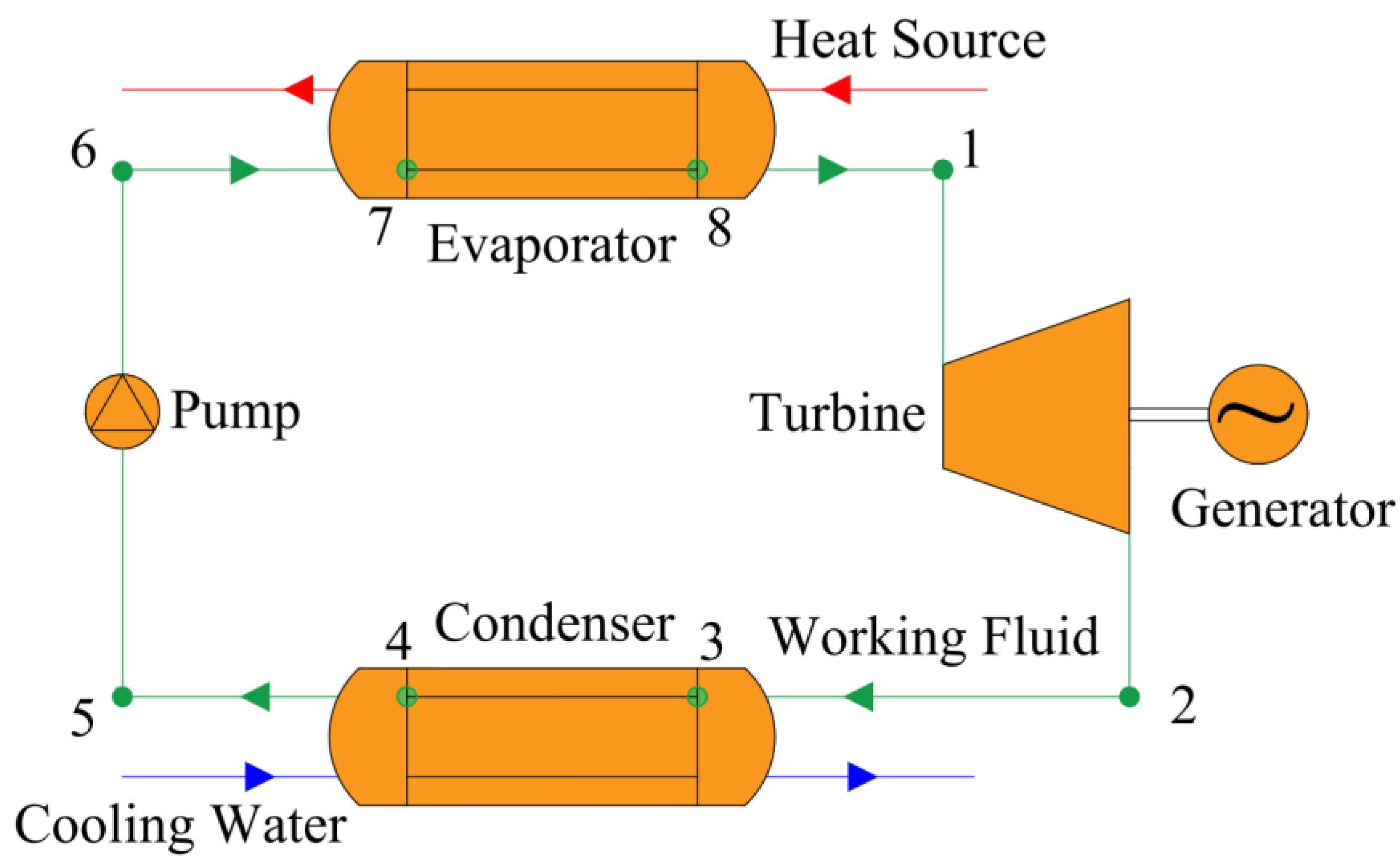
2. System Description

The ORC system consists of an evaporator, an expander, a condenser, and a pump; the schematic diagram is shown in Figure 1. Firstly, liquid–organic working fluid exchanges heat with waste heat and produces high-pressure vapor in the evaporator, and the vapor enters the expander to convert heat energy into mechanical work, which twists the generator for power generation. Cooling water in the condenser cools the vapor discharged by the expander to a liquid state. Finally, the working fluid flows from the expander to the pump to be pressurized, so it circulates continuously.

Figure 2 shows the T-s diagram of the organic Rankine cycle. Where, process 6-7-8-1 is organic working fluid heated from liquid to saturated vapor under constant pressure in the evaporator; process 1-2 is the work carried out by the working fluid in the expander; procedure 2-3-3-5 is the constant pressure cooling of the working fluid in the condenser; and process 5-6 is the working fluid pressurized by the pump.

3. Mathematical Model

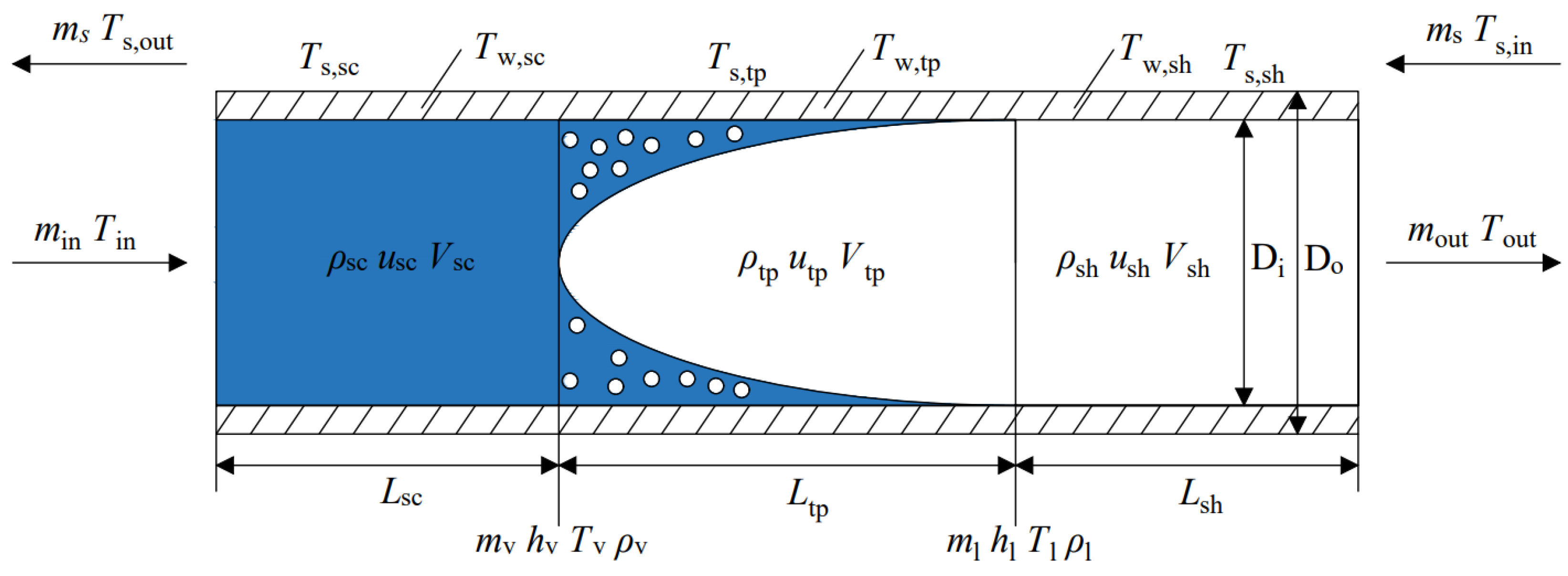
The models of the evaporator, expander, condenser, and pump were established, respectively, and the physical parameters of the working fluid and heat source were obtained. The main system parameters are shown in

Table 1. Main parameters of the dynamic ORC model.

Parameters	Unit	Value
Isentropic efficiency of the expander		0.80
Wall thickness of the evaporator	m	0.002
Outside diameter of the evaporator	m	0.4
Cylinder volume of the pump	m3	0.000045
Inside diameter of the evaporator	m	0.065
Isentropic efficiency of the pump		0.70

.

3.1. Evaporator

The establishment of the evaporator and condenser is the key in the process of building the dynamic model. The time constant of the heat exchanger is much higher than that of the expander and pump, and the dynamic response of the ORC system is mainly determined by the heat exchanger because the mechanical transient process is much faster than the heat-transfer phenomenon [30].

Two common modeling methods are the moving boundary method (MB) and finite volume method (FV) for two-phase flow heat exchangers. Both methods consist of the law of conservation of energy, mass, and momentum in heat exchangers. The results of the FV model are accurate, but the computational efficiency is lower than that of the MB method. The lumped parameter method is used to reduce the order of the MB model and improve the calculation efficiency, and the calculation accuracy is close to the FV model [31]. Therefore, the MB method was used to model the exchangers in this study.

According to the state of the working fluid, the heat exchanger can be divided into three regions: the subcooled zone, the two-phase zone, and the superheated zone by the MB model. In the simulation, the size of the region varies with the boundary of saturated liquid and saturated vapor, and the evaporator moving boundary model is shown in Figure 3. Some assumptions were made as follows before establishing the model [32].

(1)

The evaporator is defined as a horizontal cylindrical tube with a constant cross-sectional area.

(2)

The flow of working fluid and heat source in evaporator is horizontal, without vertical flow.

(3)

The pressure drop of the working fluid in the evaporator is negligible and the pressure in the tube is uniform.

(4)

The two-phase flow of the working fluid in the evaporator is uniform.

(5)

The kinetic energy as well as the gravitational potential energy of the working fluid in the evaporator are neglected.

(6)

Axial heat conduction of the working fluid and tube is ignored.

In a practical system, the pressure drop of evaporator will affect the actual operation of the system. However, if the pressure drop is considered in the MB model, the momentum conservation equation needs to be added, which will greatly increase the calculation amount of the model and reduce the robustness of the model. The MB method is widely used in evaporator dynamic modeling and provides the right trends, although the specific values are different from the experimental results [33].

The differential conservation equations were established for each region, based on the abovementioned assumptions. The mass conservation equation on the working fluid (WF) side is as follows:

$${\rho }_{\mathrm{i}}\frac{d{V}_{\mathrm{i}}}{dt}+V_{\mathrm{i}}\frac{d{\rho }_{\mathrm{i}}}{dt}=m_{\mathrm{in}}-m_{\mathrm{out}}$$

(1)

where, ρ is the average density, V is the volume of the region, m is the mass flow rate, t is the simulation time, The subscript i stands for the sub-cooled region, two-phase region, and superheated region, and the subscript in and out are the input parameter and output parameter, respectively. The energy conservation equation of the WF side is as follows:

$$\frac{d\left({\rho }_{\mathrm{i}}{u}_{\mathrm{i}}{V}_{\mathrm{i}}\right)}{dt}=m_{\mathrm{in}}{h}_{\mathrm{in}}-m_{\mathrm{out}}{h}_{\mathrm{out}}+Q_{\mathrm{i}}$$

(2)

where, u is the specific internal energy, h is the specific enthalpy, and Q is the heat quantity.

(1)

Sub-cooled region model

Since there is no phase transition in the sub-cooled region of the evaporator, the following equations can be obtained.

$$\begin{array}{c}{\rho }_{\mathrm{sc}}={\rho }_{\mathrm{sc}}\left(p,h_{\mathrm{sc}}\right)\\ u_{\mathrm{sc}}=u_{\mathrm{sc}}\left(p,h_{\mathrm{sc}}\right)\\ h_{\mathrm{v}}=h_{\mathrm{v}}(p)\\ h_{\mathrm{sc}}=\left(h_{\mathrm{in}}+h_{\mathrm{v}}\right)/2\end{array}$$

(3)

where, p is the pressure, and the subscript v and sc stand for the saturated liquid and the sub-cooled region, respectively. The following equation is obtained by deriving the above equation and bringing it into Equations (1) and (2):

$${\rho }_{\mathrm{sc}}\frac{d{V}_{\mathrm{sc}}}{dt}+V_{\mathrm{sc}}\left[\frac{dp}{dt}\left({\frac{\partial {\rho }_{\mathrm{sc}}}{\partial p}|}_{h_{\mathrm{sc}}}+{\frac{1}{2}\frac{\partial {\rho }_{\mathrm{sc}}}{\partial h_{\mathrm{sc}}}|}_P\frac{d{h}_{\mathrm{v}}}{dp}\right)+{\frac{1}{2}\frac{\partial {\rho }_{\mathrm{sc}}}{\partial h_{\mathrm{sc}}}|}_P\frac{d{h}_{\mathrm{in}}}{dt}\right]=m_{\mathrm{in}}-m_{\mathrm{v}}$$

(4)

$$\begin{array}{c}{\rho }_{\mathrm{sc}}{u}_{\mathrm{sc}}\frac{d{V}_{\mathrm{sc}}}{dt}+V_{\mathrm{sc}}\left\{\begin{array}{l}{\rho }_{\mathrm{sc}}\left[\frac{dp}{dt}\left({\frac{\partial u_{\mathrm{sc}}}{\partial p}|}_{h_{\mathrm{sc}}}+{\frac{1}{2}\frac{\partial u_{\mathrm{sc}}}{\partial h_{\mathrm{sc}}}|}_P\frac{d{h}_{\mathrm{v}}}{dp}\right)+{\frac{1}{2}\frac{d{h}_{\mathrm{in}}}{dt}\frac{\partial u_{\mathrm{sc}}}{\partial h_{\mathrm{sc}}}|}_p\right]\hfill \\ +u_{\mathrm{sc}}\left[\frac{dp}{dt}\left({\frac{\partial {\rho }_{\mathrm{sc}}}{\partial p}|}_{h_{\mathrm{sc}}}+{\frac{1}{2}\frac{\partial {\rho }_{\mathrm{sc}}}{\partial h_{\mathrm{sc}}}|}_P\frac{d{h}_{\mathrm{v}}}{dp}\right)+{\frac{1}{2}\frac{\partial {\rho }_{\mathrm{sc}}}{\partial h_{\mathrm{sc}}}|}_P\frac{d{h}_{\mathrm{in}}}{dt}\right]\hfill \end{array}\right\}\\ =m_{\mathrm{in}}{h}_{\mathrm{in}}-m_{\mathrm{v}}{h}_{\mathrm{v}}+Q_{\mathrm{sc}}\end{array}$$

(5)

The energy-balance equation and heat-transfer equation of the wall are as follows:

$$M_{\mathrm{w},\mathrm{sc}}{c}_{\mathrm{w},\mathrm{sc}}\frac{d{T}_{\mathrm{w},\mathrm{sc}}}{dt}=K_{\mathrm{s},\mathrm{sc}}{A}_{\mathrm{s},\mathrm{sc}}\left(T_{\mathrm{s},\mathrm{sc}}-T_{\mathrm{w},\mathrm{sc}}\right)-K_{\mathrm{sc}}{A}_{\mathrm{sc}}\left(T_{\mathrm{w},\mathrm{sc}}-T_{\mathrm{sc}}\right)$$

(6)

where, M is the quantity, c is the specific heat, T is the temperature, A is the heat-exchange area, K is the heat-transfer coefficient, and the subscript s and w stand for the heat source and the wall, respectively.

(2)

Two-phase region model

The average density and enthalpy of the WF in the two-phase region are expressed as follows:

$$\begin{array}{c}{\rho }_{\mathrm{tp}}=\gamma {\rho }_{\mathrm{l}}+(1-\gamma ){\rho }_{\mathrm{v}}\\ {\rho }_{\mathrm{tp}}{u}_{\mathrm{tp}}=\gamma {\rho }_{\mathrm{l}}{u}_{\mathrm{l}}+(1-\gamma ){\rho }_{\mathrm{v}}{u}_{\mathrm{v}}\end{array}$$

(7)

where, the subscript l and tp stand saturated vapor point and the two-phase region respectively, and γ is the void ratio and its expression is as follows [34]:

$$\gamma =1-\frac{1+{(1/\mu )}^{2/3}[2/3\ln (1/\mu )-1]}{{\left[{(1/\mu )}^{2/3}-1\right]}^2}$$

(8)

where, μ is the density ratio, and its expression is as follows:

$$\mu =\frac{{\rho }_{\mathrm{v}}}{{\rho }_{\mathrm{l}}}$$

(9)

The following equations are obtained by deriving the above equation and bringing it into Equations (1) and (2):

$${\rho }_{\mathrm{tp}}\frac{d{V}_{\mathrm{tp}}}{dt}+V_{\mathrm{tp}}\gamma \frac{d{\rho }_{\mathrm{l}}}{dp}+(1-\gamma )\frac{d{\rho }_{\mathrm{v}}}{dp}\frac{dp}{dt}=m_{\mathrm{v}}-m_1$$

(10)

$${\rho }_{\mathrm{tp}}{u}_{\mathrm{tp}}\frac{d{V}_{\mathrm{tp}}}{dt}+V_{\mathrm{tp}}\gamma \frac{d{\rho }_{\mathrm{l}}{u}_{\mathrm{l}}}{dp}+(1-\gamma )\frac{d{\rho }_{\mathrm{v}}{u}_{\mathrm{v}}}{dp}\frac{dp}{dt}=m_{\mathrm{v}}{h}_{\mathrm{v}}-m_{\mathrm{l}}{h}_1+Q_{\mathrm{tp}}$$

(11)

The energy-balance equation and heat-transfer equation of the wall are as follows:

$$M_{\mathrm{w},\mathrm{tp}}{\mathrm{c}}_{\mathrm{W},\mathrm{tp}}\frac{d{T}_{\mathrm{w},\mathrm{tp}}}{dt}=K_{\mathrm{s},\mathrm{tp}}{A}_{\mathrm{s},\mathrm{tp}}\left(T_{\mathrm{s},\mathrm{tp}}-T_{\mathrm{w},\mathrm{tp}}\right)-K_{\mathrm{tp}}{A}_{\mathrm{tp}}\left(T_{\mathrm{w},\mathrm{tp}}-T_{\mathrm{tp}}\right)$$

(12)

(3)

Superheat region model

Since there is no same-phase transition in the superheated region, the mass and energy conservation equations of the WF are as follows:

$${\rho }_{\mathrm{sh}}\frac{d{V}_{\mathrm{sh}}}{dt}+V_{\mathrm{sh}}\left[\frac{dp}{dt}\left({\frac{\partial {\rho }_{\mathrm{sh}}}{\partial p}|}_{h_{\mathrm{sh}}}+{\frac{1}{2}\frac{\partial {\rho }_{\mathrm{sh}}}{\partial h_{\mathrm{sh}}}|}_p\frac{d{h}_1}{dp}\right)+{\frac{1}{2}\frac{\partial {\rho }_{\mathrm{sh}}}{\partial h_{\mathrm{sh}}}|}_p\frac{d{h}_{\mathrm{out}}}{dt}\right]=m_1-m_{\mathrm{out}}$$

(13)

$$\begin{array}{c}{V}_{\mathrm{sh}}\left\{\begin{array}{c}[u_{\mathrm{sh}}({\frac{\partial {\rho }_{\mathrm{sh}}}{\partial p}|}_{h_{\mathrm{sh}}}+{\frac{1}{2}\frac{\partial {\rho }_{\mathrm{sh}}}{\partial h_{\mathrm{sh}}}|}_p\frac{d{h}_{\mathrm{l}}}{dp})+{\rho }_{\mathrm{sh}}\left({\frac{\partial u_{\mathrm{sh}}}{\partial p}|}_{h_{\mathrm{sh}}}+{\frac{1}{2}\frac{\partial u_{\mathrm{sh}}}{\partial h_{\mathrm{sh}}}|}_p\frac{d{h}_{\mathrm{l}}}{dp}\right)]\frac{dp}{dt}\\ +\left({u_{\mathrm{sh}}\frac{1}{2}\frac{\partial {\rho }_{\mathrm{sh}}}{\partial h_{\mathrm{sh}}}|}_p+{{\rho }_{\mathrm{sh}}\frac{1}{2}\frac{\partial u_{\mathrm{sh}}}{\partial h_{\mathrm{sh}}}|}_p\right)\frac{d{h}_{\mathrm{out}}}{dt}\end{array}\right\}\\ +{\rho }_{\mathrm{sh}}{u}_{\mathrm{sh}}\frac{d{V}_{\mathrm{sh}}}{dt}=m_{\mathrm{l}}{h}_{\mathrm{l}}-m_{\mathrm{out}}{h}_{\mathrm{out}}+Q_{\mathrm{sh}}\end{array}$$

(14)

The subscript sh stands for the superheat region. The energy-balance equation and heat-transfer equation of the wall are as follows:

$$M_{\mathrm{w},\mathrm{sh}}{c}_{\mathrm{w},\mathrm{sh}}\frac{d{T}_{\mathrm{w},\mathrm{sh}}}{dt}=K_{\mathrm{s},\mathrm{sh}}{A}_{\mathrm{s},\mathrm{sh}}\left(T_{\mathrm{s},\mathrm{sh}}-T_{\mathrm{w},\mathrm{sh}}\right)-K_{\mathrm{sh}}{A}_{\mathrm{sh}}\left(T_{\mathrm{w},\mathrm{sh}}-T_{\mathrm{sh}}\right)$$

(15)

(4)

Heat source model

There is no phase transition of the heat source in the heat-transfer process of evaporator, so the change of its physical parameters is not considered. The energy-balance equation of heat source in each region of evaporator is as follows:

$$Q_{\mathrm{s},\mathrm{i}}=m_{\mathrm{s}}{c}_{\mathrm{s},\mathrm{i}}\left(T_{\mathrm{s},\mathrm{in}}-T_{\mathrm{s},\mathrm{out}}\right)$$

(16)

where, T is the temperatures, and the subscript s stands for the heat source.

(5)

Heat-transfer coefficient

The Dittus–Boelter correlation is widely used to calculate Nusselt numbers for fluids in the tube-side single-phase, as follows: [35]

$$Nu=0.023R{e}^{0.8}P{r}^{0.4}$$

(17)

where Re is the Reynolds number and Pr is the Planck number. The heat-transfer coefficient of the tube-side is expressed as follows:

$$K_{\mathrm{s},\mathrm{i}}=\frac{\lambda Nu}{d_{\mathrm{out}}}$$

(18)

where λ is the thermal conductivity. For the WF side, Heat-transfer coefficient of the single-phase region is obtained by the Gnielinski equation: [36]

$$Nu=\frac{(f/8)(Re-1000)Pr}{1+12.7\sqrt{f/8}\left(P{r}^{2/3}-1\right)}\left[1+{\left(\frac{d_{\mathrm{in}}}{L_{\mathrm{i}}}\right)}^{2/3}\right]$$

(19)

where, the friction factor f is calculated by Filonenko’s correlation:

$$f={(1.82\lg Re-1.64)}^{-2}$$

(20)

The heat-transfer coefficient in the two-phase region is calculated by the following formula:

$$\begin{array}{c}{K}_{\mathrm{tp}}=K_{\mathrm{sc}}\{{\left[(1-x)+1.2x^{0.4}(1-x){\left(\frac{{\rho }_{\mathrm{v}}}{{\rho }_{\mathrm{l}}}\right)}^{0.37}\right]}^{-2.2}\\ {+{\left[\frac{K_{\mathrm{sh}}}{K_{\mathrm{sc}}}{x}^{0.01}\left(1+8{(1-x)}^{0.7}{\left(\frac{{\rho }_{\mathrm{v}}}{{\rho }_{\mathrm{l}}}\right)}^{0.67}\right)\right]}^{-2}\}}^{-0.5}\end{array}$$

(21)

where x is the mass fraction of the gas in the two-phase region, which is expressed as:

$$x=\frac{h_{\mathrm{tp}}-h_{\mathrm{v}}}{h_{\mathrm{l}}-h_{\mathrm{v}}}$$

(22)

3.2. Condenser

The condenser is also modeled by the MB method. The WF is transferred to the saturated gas phase in the superheated region, then to the saturated liquid phase in the two-phase region, and finally passes through the sub-cooled region. The condensing pressure can be controlled by adjusting the mass flow of cooling water under the condition of constant temperature. It can be assumed that the condensing temperature and condensing pressure are constant for simplicity and a faster calculation speed, since the experimental and simulation data of [37] showed that the variation of condensing pressure is small under dynamic operation.

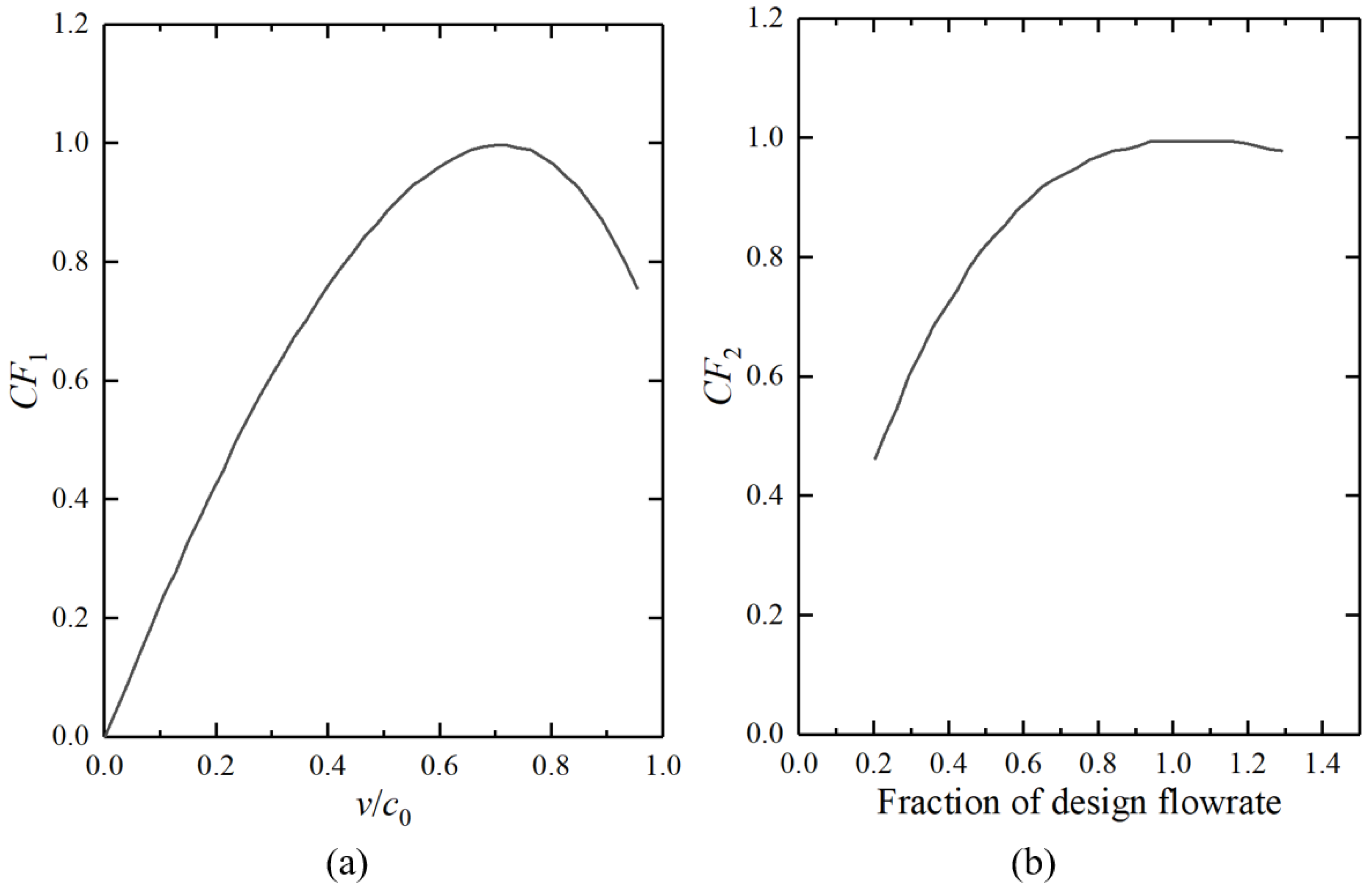
3.3. Pump and Expander

Compared with the heat exchanger, the dynamic characteristics of the expander and pump are fast, so this paper used algebraic equations to model them [38].

The mass-flow rate, outlet thermal energy, and power consumption of organic WF in the pump model are calculated by the following formula:

$$m_{\mathrm{p}}={\eta }_{\mathrm{p},\mathrm{vol}}{V}_{\mathrm{p}}{\rho }_{\mathrm{p},\mathrm{in}}{\omega }_{\mathrm{p}}$$

(23)

where, η is the efficiency, ω is the rotational speed, and the subscript p and vol stand for pump and volume, respectively.

$$h_{\mathrm{p},\mathrm{out}}=h_{\mathrm{p},\mathrm{in}}+\frac{h_{\mathrm{p},\mathrm{is}}-h_{\mathrm{p},\mathrm{in}}}{{\eta }_{\mathrm{is},\mathrm{p}}}$$

(24)

The subscript is stands for isentropic.

$$W_{\mathrm{p}}=m_{\mathrm{p}}\frac{p_{\mathrm{p},\mathrm{out}}-p_{\mathrm{p},\mathrm{in}}}{{\rho }_{\mathrm{p},\mathrm{in}}{\eta }_{\mathrm{p},\mathrm{is}}}$$

(25)

where, W is the power. The modeling equation of expander is as follows:

$$m_{\mathrm{x}}={\eta }_{\mathrm{x},\mathrm{vol}}{V}_{\mathrm{x}}{\rho }_{\mathrm{x},\mathrm{in}}{\omega }_{\mathrm{x}}$$

(26)

The subscript x stands for the expander.

$$h_{\mathrm{x},\mathrm{out}}=h_{\mathrm{x},\mathrm{in}}+{\eta }_{\mathrm{x},\mathrm{is}}\left(h_{\mathrm{x},\mathrm{is}}-h_{\mathrm{x},\mathrm{in}}\right)$$

(27)

where, η_x,is is the isentropic efficiency of the expander, which can be expressed as follows: [39]

$${\eta }_{\mathrm{x},\mathrm{is}}=C{F}_{1}C{F}_2{\eta }_{\mathrm{x},\mathrm{is}0}$$

(28)

CF₁ is related to the ratio of expansion wheel top velocity v to spray velocity c₀, and CF₂ is related to the ratio of the mass-flow rate to the design mass flow rate, as shown in Figure 4.

where, spray velocity c₀ is expressed as:

$$c_0=\sqrt{2\left(h_{\mathrm{x},\mathrm{in}}-h_{\mathrm{x},\mathrm{is}}\right)}$$

(29)

The power output of the expander and net power output of the system are as follows:

$$W_{\mathrm{x}}=\left(h_{\mathrm{x},\mathrm{in}}-h_{\mathrm{x},\mathrm{out}}\right){\eta }_{\mathrm{x}}{m}_{\mathrm{x}}$$

(30)

$$W_{\mathrm{net}}=W_{\mathrm{x}}-W_{\mathrm{p}}$$

(31)

The subscript net stands for net output, and the thermal efficiency is calculated by the following formula:

$${\eta }_{th}=W_{\mathrm{net}}/Q_{\mathrm{e}}$$

(32)

where, Q is the heat exchange of working fluid, and the subscript e and th stand for the evaporator and thermal, respectively.

$${\eta }_{\mathrm{ex}}=W_{\mathrm{net}}/E_{\mathrm{in}}$$

(33)

where, E and the subscript ex both stand for exergy.

3.4. Model Solution

The dynamic model of the main components was established at first, and then the system model was established by proper combination according to the relationship between the component models. For ORC system modeling, the relationship between each component is shown in Figure 5. It can be found that input parameters of the whole model were the temperature and mass-flow rate of the heat source and cooling water. All parameters and equations were coupled with each other to become a closed loop so as to obtain the unique solution of the model. In this study, MATLAB and an ode15 s solver were used for programming and solving. The physical parameters of the organic working fluid were obtained by calling REFPROP.

4. Validation

The modeling method of the dynamic model is consistent with that of reference [33]. The parameters were set in accordance with the literature to verify the accuracy of the dynamic model.

The p_e of the simulation results and the length of each phase region were compared with the results of the references as shown in the Figure 6. During the simulation, the pump speed increased by 5% at t = 0 s. The external heat-transfer coefficient increased by10% at 30 s. Finally, the nozzle coefficient increased by 10% at 60 s. The simulation results are very close to those of the literature. This proves the accuracy of the dynamic model established in this paper. The reason for the small difference between the results is that the error of the iterative algorithm used in the literature is different from that in this paper. A larger allowable error was adopted in the model of this study for obtain better robustness. It can be found from Figure 6 that this operation did not affect the accuracy of the model.

5. Results and Discussion

This paper focused on the dynamic performance of ORC driven by low-temperature waste heat. The temperature below 473.15 K is called low-temperature industrial waste heat, so the average heat-source temperature was set as 448.15 K and the mass flow rate was set as 0.5 kg/s. The low-temperature ORC with R245fa as the WF has high circulation efficiency, so R245fa was used as the WF of the system [40].

In practical engineering, waste heat fluctuates under different amplitudes and periods. The general results of dynamic behavior of ORC system driven by fluctuating residual heat are obtained by setting T_s as a sine function. The T_s fluctuates as follows:

$$T_{\mathrm{s}}=T_{\mathrm{avg}}+\mathsf{\Delta }T\sin \frac{2\pi t}{P_{\mathrm{f}}}$$

(34)

where, A_f is the amplitude, P_f is the period, the subscript AVG stands for the average value. In this section, the effects of sinusoidal T_s on the dynamic response performance of the basic ORC system were evaluated and the evaporating pressure (p_e), net power output (W_net), thermal efficiency (η_th), exergy efficiency (η_ex) and superheat degree (SH) were analyzed. On the basis of SH = 30 K steady-state heat source, the temperature of the sine heat source fluctuated when the amplitude was ∆T_s = 5 K, 10 K and 15 K, and the fluctuation period was 20 min, 25 min, and 30 min, respectively, to ensure the normal operation of the dynamic model. The operating parameters and power-generation performance of the system under the steady-state heat source are shown in

Table 2. Main parameters under the steady-state heat source.

Parameters	Unit	Value
Heat-source temperature	K	448.15
Heat source mass-flow rate	kg/s	0.50
Evaporating pressure	kPa	1350.99
Working fluid mass-flow rate	kg/s	0.82
Superheat degree	K	30.00
Condensing pressure	kPa	148.25
Net power output	kW	29.55
Length of the evaporator	m	102.42
Thermal efficiency	%	12.80
Exergy efficiency	%	48.26

.

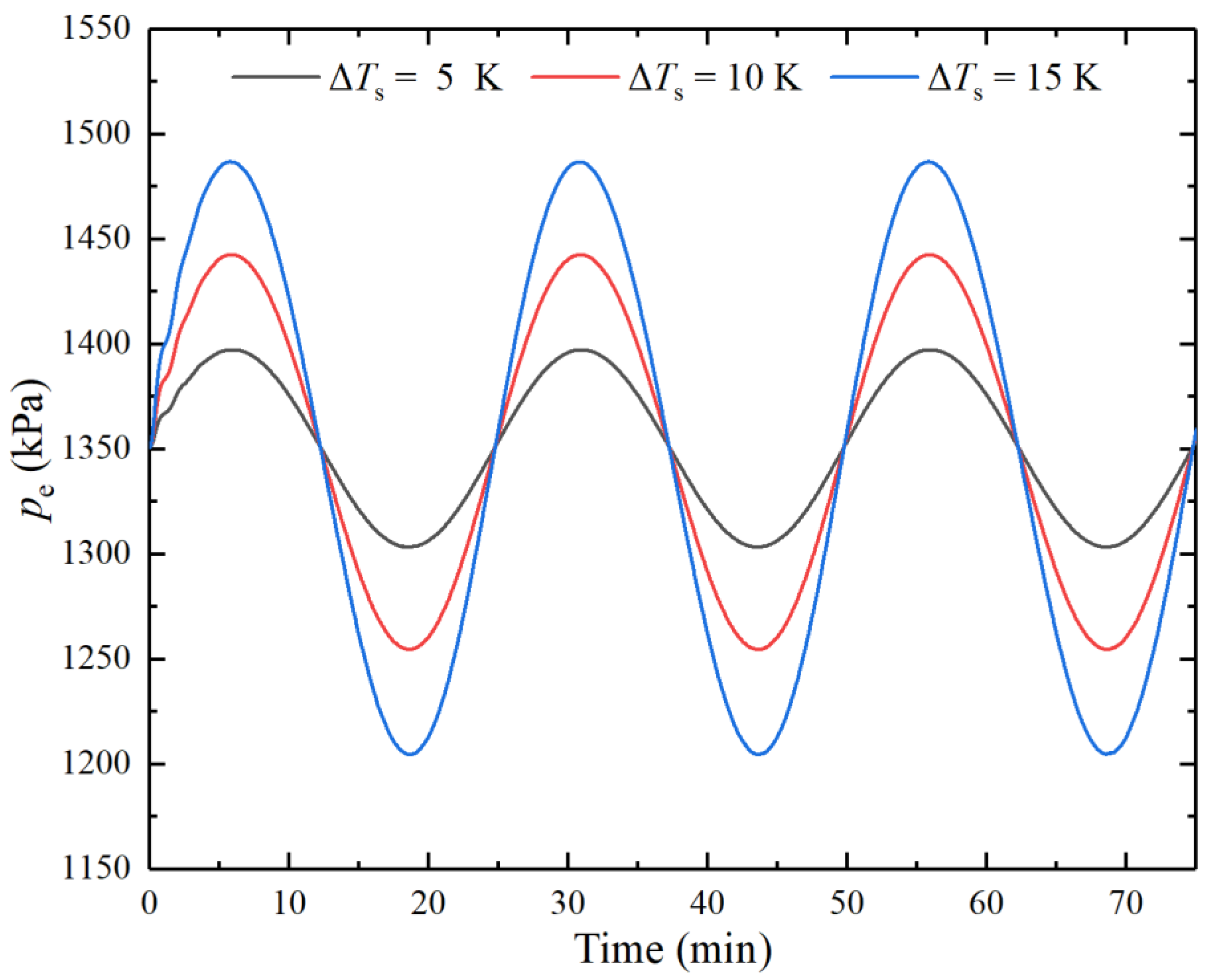
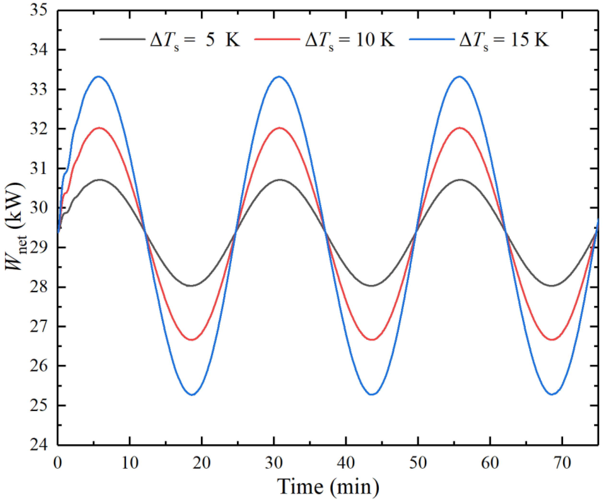
5.1. Influence of Fluctuating Heat-Source Temperature

The effect of sinusoidal T_s on the dynamic response performance of the ORC system was studied. Where, the heat source amplitudes were set as ∆T_s = 5 K, 10 K, and 15 K, and the fluctuation period was set as 25 min.

Figure 7 shows the dynamic response of p_e under different amplitudes. The results showed that the change of p_e was approximately sinusoidal and was the same as that of the heat source. The p_e increased with the increase of amplitude. The reason is that when the temperature rises, the WF in the evaporator absorbs more heat and generates more saturated vapor, resulting in a rapid increase of p_e. At the early stage of the model operation, the p_e showed irregular changes. The reason is that the T_s changed at the same time of the system operation, and the system was not stable. The maximum values of p_e were 1397.37 kPa, 1442.65 kPa, and 1486.91 kPa, and the average values were 1350.66 kPa, 1349.67 kPa, and 1348.02 kPa, respectively. The maximum value of p_e increased with the increase of amplitude, but its average value decreased with the increase of amplitude and was less than the steady-state value. This indicates that the increase of T_s has less influence on p_e than the decrease of T_s.

From Figure 8, the dynamic response of the W_net showed the same trend as the p_e, the change of it showed a sinusoidal trend, and the dynamic response was unstable at any fixed fluctuating amplitude. The amplitude of the W_net increased with the increase of the T_s amplitude. The reason is that when the temperature rises, the heat transfer of the WF in the evaporator increases, and the enthalpy into the expander will increase, thus increasing the W_net. The average values of the W_net under the three amplitudes were 29.38 kW, 29.36 kW, and 29.33 kW, respectively, which are all less than the W_net of the ORC system under the steady-state condition, and that is negative correlated with the amplitude. The fluctuation of T_s will make the density of the WF at the outlet of the evaporator fluctuate, thus changing the mass-flow rate of the expander, and it will affect the isentropic efficiency of the expander.

Figure 9 shows the dynamic response of η_th under different amplitude, which is the same as the variation trend of p_e and W_net. It can be found that the instability of η_th is increased in the first cycle. The reason is that the heat transfer in the evaporator fluctuated with small amplitude in the first cycle, and the η_th is the ratio of the W_net to it. The average thermal efficiencies of the three amplitudes were 12.72%, 12.71%, and 12.69%, respectively, which are all less than the steady-state value and negatively correlated with the amplitude.

The variation trend of η_ex under sinusoidal the heat source is opposite to that of the heat source, which is shown in Figure 10. The reason is that the heat source pressure increases with the increase of T_s, and exergy is affected by both temperature and pressure, which leads to the increase of exergy into the system. Under the three amplitudes, the average exergy efficiencies were 47.99%, 47.96%, and 47.93%, respectively. The average values decreased with the increase of amplitude and were lower than the steady-state value.

When the heat source fluctuates greatly, the WF cannot be completely evaporated in the evaporator, which will damage the expander. Therefore, the SH in the evaporator must be kept above 0 during the operation of ORC system. Figure 11 shows the effect of fluctuation amplitude on SH when the period = 25 min. It can be found that when the T_s fluctuated, the fluctuation trend of the SH was consistent with that of the heat source. Different from the p_e, the average values of the SH under the three amplitudes were 30.01 K, 30.03 K, and 30.05 K, respectively, which are all larger than the steady-state value of the SH.

In summary, the fluctuation of system operating parameters and generation performance increased with the increase of the amplitude of the fluctuating heat source, and the average value was negatively proportional to the amplitude. The dynamic characteristics of system operating parameters and power-generation performance were affected by the amplitude of heat-source temperature, so reducing the amplitude is the key in industrial waste heat pretreatment projects.

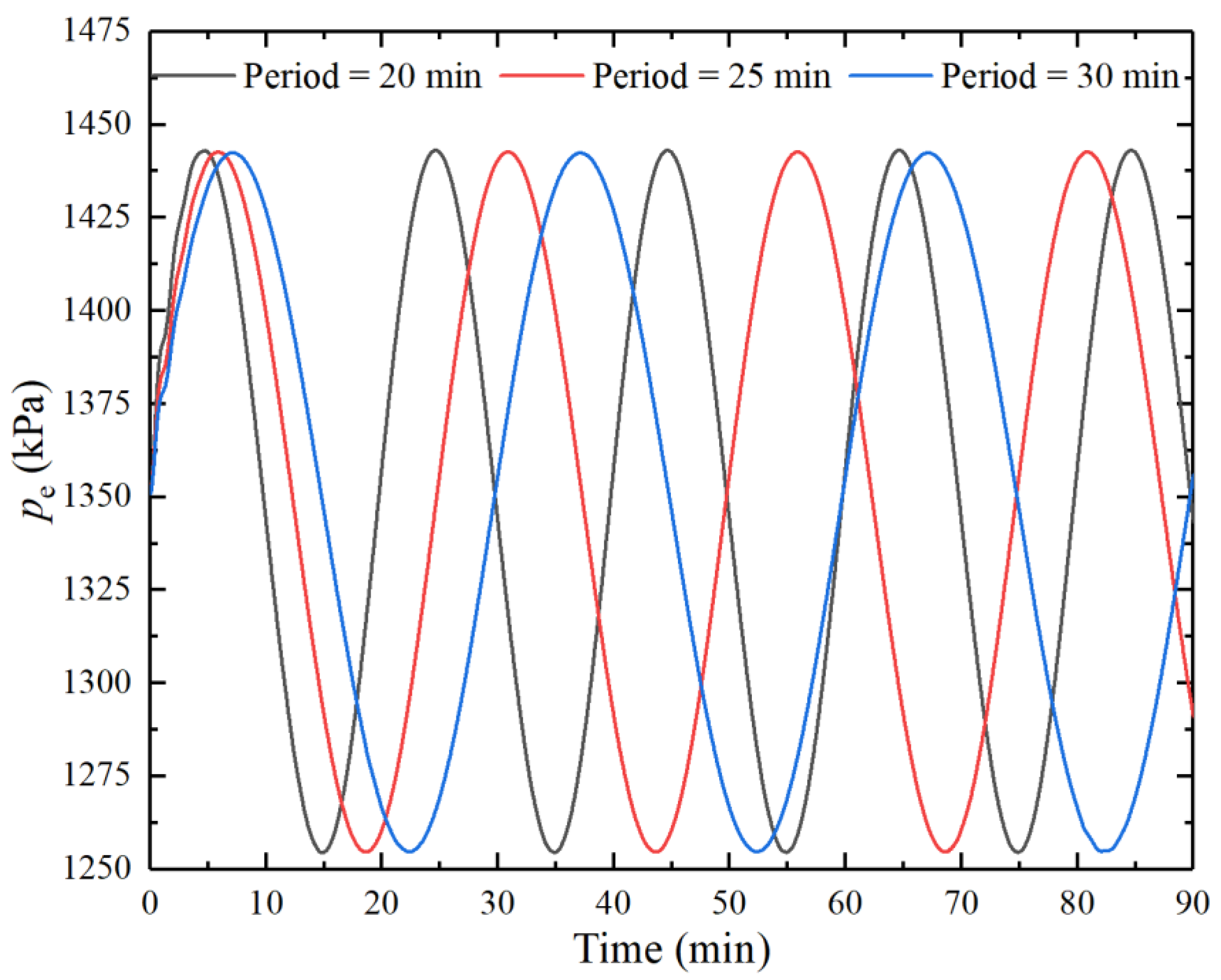
5.2. Influence of Heat Source Period

In this section, the relationship between dynamic performance and period of the fluctuating heat source was studied. In practical engineering, the fluctuation period of industrial waste heat is about 25 min [41]. Therefore, the amplitude of T_s was 10 K, and the periods were 20 min, 25 min and 30 min.

From Figure 12, the fluctuation trends of p_e under different fluctuation periods were basically consistent with that of T_s, and the extreme values under the three periods were almost equal. The second peak of p_e occurred at 25.35 min, 31.65 min, and 37.95 min, respectively, while that of T_s occurred at 25.00 min, 31.25 min, and 37.50 min, respectively. The peak of p_e appeared later than that of the T_s; the reason is when the temperature of the heat source fluctuates to the peak, the heat absorption of the WF does not reach the peak, and the heat transfer between that has a certain response time. The time difference between the peak of p_e and T_s was proportional to the fluctuation period.

Identically to p_e, the fluctuation trend of W_net was almost the same as that of the heat source, shown in Figure 13. The second peak of W_net occurred at 25.45 min, 31.7 min, and 38.00 min, respectively, which is not only later than that of T_s, but also later than the p_e, because the saturated vapor into the expansion machine to do work requires a certain response time. The average value of W_net under the three periods was 29.36 kW, which is lower than that in the steady state, indicating that heat source fluctuation is not conducive to the W_net, and the influence of fluctuation period on the average value can be ignored. It can be found that this conclusion is the same as in Section 5.1. W_net fluctuated erratically in the first period for two reasons: firstly, the operating parameters of the system begin to change in the initial stage. At this time, the iteration of physical quantities led to oscillation in the first cycle. Secondly, the W_net was derived from the W_x and the W_p, and there is a certain difference in response time between the two.

Figure 14 shows the dynamic response of η_th under three periods. The fluctuation of η_th was irregular at the initial stage, because the η_th is the ratio of W_net to the heat absorption of WF, and the response time of the two was different and it can be found that this phenomenon also occurred when the temperature of the heat source dropped to the trough. The iteration of parameters also resulted in this phenomenon when the T_s changed. The fluctuation range of η_th was inversely proportional to the period, and the reason is that the increase of the period will lead to the increase of the heat absorption of the WF. The average value of η_th under the three cycles was 12.71%, indicating that the fluctuation of the T_s is not conducive to the η_th.

The relationship between SH and periods is shown in Figure 15. Its fluctuation trend was consistent with the T_s, and the fluctuation range was almost the same under the three periods. The second peak of SH occurred at 25.3 min, 31.55 min, and 37.8 min, respectively, under the three cycles, which are later than that of the T_s, but earlier than that of p_e. The reason is that the increase of SH leads to the increase of saturated vapor and thus the increase of p_e, so there is a certain time difference between the SH and p_e. To sum up, the operating parameters of the system have a certain response time, and the response time increases with the increase of the period. When the fluctuation period is large, the temperature fluctuation of heat source will lead to the decrease of the average power-generation performance of the system.

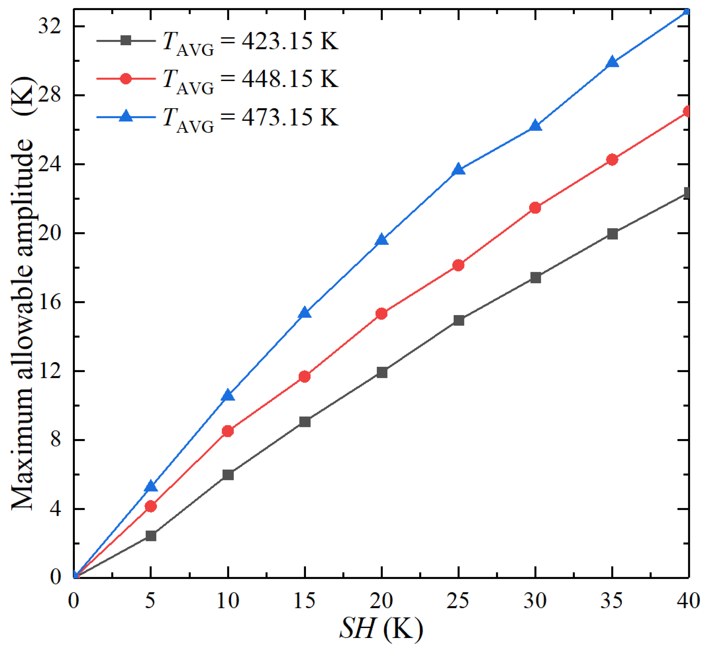
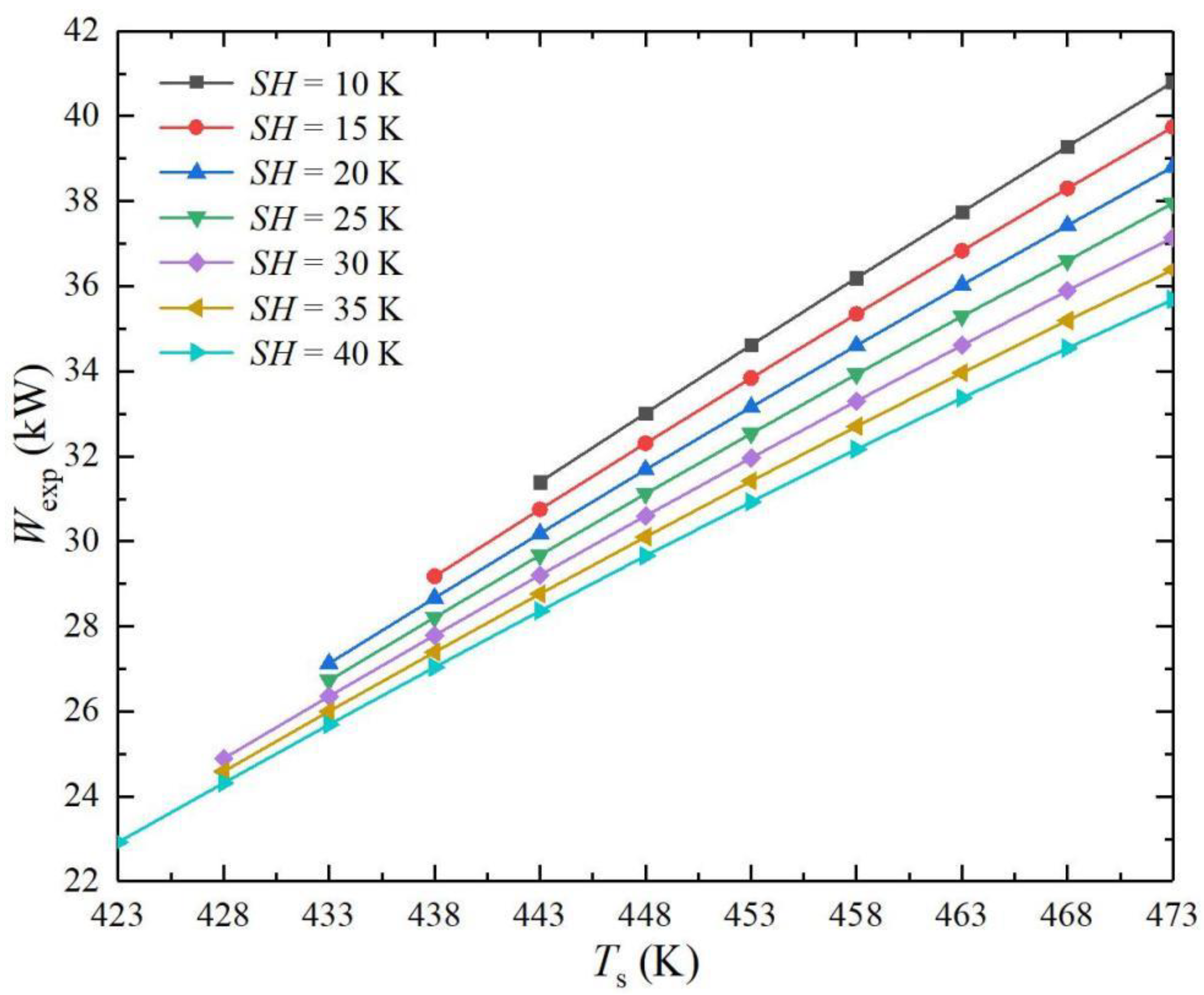
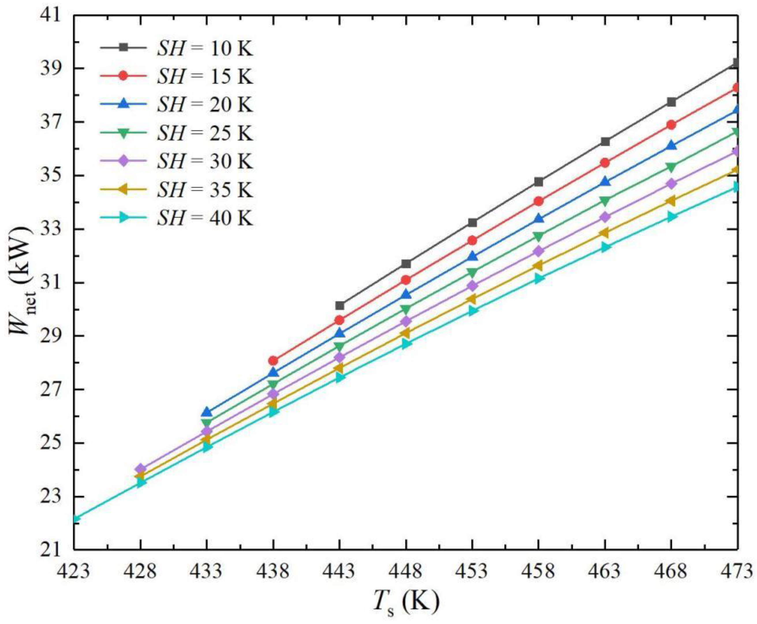
5.3. Influence of Superheat Degree

Under the condition of a pulsating heat source, the operation of the system needs special attention. When the T_s drops substantially, the heat absorption of the WF in the evaporator will be reduced, and the superheated region will disappear. The two-phase WF will go directly into the expander. Unsaturated wet vapor can easily cause liquid shock in the expander, which seriously affects the operation safety of the unit. Therefore, the minimum SH was defined as SH_min, and SH_min > 0 was defined as the condition for determining system safety. When the system uses a screw expander, the WF at the inlet of the expander can be wet vapor. However, in order to make the conclusions of this study applicable to different situations, we took SH as the key factor to evaluate the safety of the system.

T_s has a large impact on system safety, and industrial waste heat fluctuates under a long period. SH should be set in the initial design of evaporator to deal with the disappearance of superheated region caused by T_s fluctuation. Therefore, Figure 16 shows the relationship between the maximum allowable amplitude and SH of the system after a full response. For the generality of the conclusion, the relationship between the maximum allowable amplitude and SH was studied when T_s = 423.15 K, 448.15 K, and 473.15 K. It can be found that the maximum allowable amplitude was approximately linear with the SH, and the slope increased with the increase of the average T_s. Therefore, system safety is directly proportional to the average T_s and SH.

The influence of T_s and SH on the operation of the system is discussed in this section. In order to avoid the two-phase state of the WF entering the expander, the working conditions were divided into the following categories according to the difference of SH, as shown in

Table 3. Operation parameters of the ORC system under different superheat degrees.

Parameters	Working Fluid Flow Rate, kg/s	Evaporating Pressure, kPa
SH = 10 K	0.92	1473.02
SH = 15 K	0.90	1411.01
SH = 20 K	0.87	1380.78
SH = 25 K	0.84	1365.81
SH = 30 K	0.82	1350.99
SH = 35 K	0.80	1321.72
SH = 40 K	0.78	1293.47

. The data in the table were optimized from the steady-state model.

The performance of the system with T_s between 423.15 K and 473.15 K is analyzed from five aspects: p_e, W_exp, W_net, η_th, and η_ex.

Figure 17 shows the relationship between T_s and p_e under different SH. It can be found that the p_e increased with the increase of the T_s, because the increase of the T_s led to the increase of the heat transfer of the WF and saturated vapor in the evaporator. When SH = 10 K, the p_e was always higher than other conditions; the reason is that when T_s remains constant, the increase of SH will increase the length of the superheat region in the evaporator, which will lead to the decrease of heat source side temperature in the two-phase region, thus reducing the evaporation temperature. It can be concluded that the p_e is inversely proportional to the SH and directly proportional to the T_s and the slope of the curve decreases with the increase of T_s.

The curve of the relationship between the W_exp and the temperature of the heat source at different SH is shown in Figure 18. It can be found that the W_exp was directly proportional to the T_s and inversely proportional to the SH. Although the increase of SH can increase the enthalpy difference between the inlet and outlet of the expander, it will also reduce the mass flow rate of the WF, as shown in Table 3. The reason is that the decrease of mass flow rate leads to a longer heat exchange time between the WF and the heat source in the evaporator, the increase of heat exchange and the increase of SH. When the SH decreased from 40 K to 10 K, and the output power of the expander increased by 11.32% at T_s = 448.15 K. Therefore, lower SH is more conducive to the power output of the system.

The relationship between the W_net and the T_s is shown in Figure 19, which has the same trend as the expansion work. The work consumption of the WF pump is related to the outlet enthalpy of the condenser, but the effect of the condenser on the system is not considered in this study. The SH decreased from 40 K to 10 K, and the net power increased by 10.47% at T_s = 448.15 K. From the point of view of output work, whether the output work of expansion or W_net, output work and SH are inversely proportional.

Figure 20 shows the relationship between η_th and T_s under different SH. The η_th was directly proportional to the T_s and inversely proportional to the SH, and the slope of the curve decreased with the increase of the T_s. The reason is that the heat exchange of the system increases with the increase of the T_s, and its variation is larger than the W_net, and the η_th is the ratio of W_net to heat transfer. When the SH decreased from 40 K to 10 K, the η_th increased by 4.9% at T_s = 448.15 K.

The relationship between η_ex of the system and T_s is shown in Figure 21. It can be found that the η_ex of the system was inversely proportional to the T_s and SH. The reason is that the heat source pressure increases with the increase of T_s, and exergy is affected by both temperature and pressure, which leads to the increase of exergy into the system. When the SH decreased from 40 K to 10 K, the η_ex increased by 10.47% at T_s = 448.15 K.

The analysis of p_e, the W_exp, W_net, η_th, and η_ex showed that T_s was inversely proportional to η_ex and proportional to other parameters, all of which were inversely proportional to SH. Therefore, the SH of the system should be reduced as far as possible. When designing the operating condition of the system, the temperature variation range of the heat source can be predicted first, and then the SH of the WF in the evaporator can be calculated by the fitting formula. On this basis, the initial setting of the SH can be adjusted. However, if the screw expander is used in the ORC system, the inlet WF can be wet vapor.

6. Conclusions

The dynamic model of the Organic Rankine cycle (ORC) system was established to study the dynamic performance under fluctuating waste heat. The amplitudes, periods of fluctuating heat source, and superheat degree were considered comprehensively, and their effects on system performance and operation were studied. The main conclusions are summarized as follows. The effect of amplitude and period of fluctuating heat source on power-generation performance can be extended to the basic ORC systems driven by single organic working medium. When the temperature of the reservoir is different, the conclusion is still applicable. Scholars can design the control system and component parameters of the system according to the conclusions of this paper.

(1)

The fluctuation of system operating parameters and generating performance are proportional to the heat source amplitude, and their average is inversely proportional to the amplitude. The fluctuation of heat-source temperature will degrade power-generation performance at any amplitude. The amplitude of heat source has a large influence on the system and reducing it is particularly key in industrial waste-heat pretreatment engineering.

(2)

The operating parameters of the system have a certain response time, and that is proportional to the period. The extreme values of the operating parameters and net power output are independent of the period, but the amplitude of the thermal efficiency is inversely proportional to the period. The fluctuating heat source resulted in reduction of the average generation performance with any period.

(3)

The maximum allowable range of the amplitude is proportional to the average temperature and superheat degree. The increase of superheat degree will reduce the power-generation performance, but improve the adaptability of the system. Under any superheat degree, the net power output and thermal efficiency are proportional to the heat-source temperature, while the exergy efficiency is inversely proportional to the heat-source temperature.

References

1. Mahmoudi, A.; Fazli, M.; Morad, M.R. A Recent Review of Waste Heat Recovery by Organic Rankine Cycle. Appl. Therm. Eng. 2018, 143, 660–675. [Google Scholar] [CrossRef]
2. Woudstra, N.; Woudstra, T.; Pirone, A.; van der Stelt, T. Thermodynamic Evaluation of Combined Cycle Plants. Energy Convers. Manag. 2010, 51, 1099–1110. [Google Scholar] [CrossRef]
3. Tchanche, B.F.; Lambrinos, G.; Frangoudakis, A.; Papadakis, G. Low-Grade Heat Conversion into Power Using Organic Rankine Cycles–A Review of Various Applications. Renew. Sustain. Energy Rev. 2011, 15, 3963–3979. [Google Scholar] [CrossRef]
4. Wang, T.; Zhang, Y.; Peng, Z.; Shu, G. A Review of Researches on Thermal Exhaust Heat Recovery with Rankine Cycle. Renew. Sustain. Energy Rev. 2011, 15, 2862–2871. [Google Scholar] [CrossRef]
5. Wang, J.; Dai, Y.; Gao, L. Exergy Analyses and Parametric Optimizations for Different Cogeneration Power Plants in Cement Industry. Appl. Energy 2009, 86, 941–948. [Google Scholar] [CrossRef]
6. Hung, T.C.; Shai, T.Y.; Wang, S.K. A Review of Organic Rankine Cycles (ORCs) for the Recovery of Low-Grade Waste Heat. Energy 1997, 22, 661–667. [Google Scholar] [CrossRef]
7. Bahrami, M.; Pourfayaz, F.; Kasaeian, A. Low Global Warming Potential (GWP) Working Fluids (WFs) for Organic Rankine Cycle (ORC) Applications. Energy Rep. 2022, 8, 2976–2988. [Google Scholar] [CrossRef]
8. Chen, X.; Liu, C.; Li, Q.; Wang, X.; Xu, X. Dynamic Analysis and Control Strategies of Organic Rankine Cycle System for Waste Heat Recovery Using Zeotropic Mixture as Working Fluid. Energy Convers. Manag. 2019, 192, 321–334. [Google Scholar] [CrossRef]
9. Wu, X.; Chen, J.; Xie, L. Fast Economic Nonlinear Model Predictive Control Strategy of Organic Rankine Cycle for Waste Heat Recovery: Simulation-Based Studies. Energy 2019, 180, 520–534. [Google Scholar] [CrossRef]
10. Hu, B.; Guo, J.; Yang, Y.; Shao, Y. Selection of Working Fluid for Organic Rankine Cycle Used in Low Temperature Geothermal Power Plant. Energy Rep. 2022, 8, 179–186. [Google Scholar] [CrossRef]
11. Tchanche, B.F.; Papadakis, G.; Lambrinos, G.; Frangoudakis, A. Fluid Selection for a Low-Temperature Solar Organic Rankine Cycle. Appl. Therm. Eng. 2009, 29, 2468–2476. [Google Scholar] [CrossRef] [Green Version]
12. Li, D.; Zhang, S.; Wang, G. Selection of Organic Rankine Cycle Working Fluids in the Low-Temperature Waste Heat Utilization. J. Hydrodyn. Ser. B 2015, 27, 458–464. [Google Scholar] [CrossRef]
13. Liang, Z.; Liang, Y.; Luo, X.; Chen, J.; Yang, Z.; Wang, C.; Chen, Y. Superstructure-Based Mixed-Integer Nonlinear Programming Framework for Hybrid Heat Sources Driven Organic Rankine Cycle Optimization. Appl. Energy 2022, 307, 118277. [Google Scholar] [CrossRef]
14. Rad, E.A.; Mohammadi, S.; Tayyeban, E. Simultaneous Optimization of Working Fluid and Boiler Pressure in an Organic Rankine Cycle for Different Heat Source Temperatures. Energy 2020, 194, 116856. [Google Scholar] [CrossRef]
15. Wang, Q.; Wang, J.; Li, T.; Meng, N. Techno-Economic Performance of Two-Stage Series Evaporation Organic Rankine Cycle with Dual-Level Heat Sources. Appl. Therm. Eng. 2020, 171, 115078. [Google Scholar] [CrossRef]
16. Pili, R.; Jørgensen, S.B.; Haglind, F. Multi-Objective Optimization of Organic Rankine Cycle Systems Considering Their Dynamic Performance. Energy 2022, 246, 123345. [Google Scholar] [CrossRef]
17. Yu, X.; Huang, Y.; Li, Z.; Huang, R.; Chang, J.; Wang, L. Characterization Analysis of Dynamic Behavior of Basic ORC under Fluctuating Heat Source. Appl. Therm. Eng. 2021, 189, 116695. [Google Scholar] [CrossRef]
18. Shu, G.; Wang, X.; Tian, H.; Liu, P.; Jing, D.; Li, X. Scan of Working Fluids Based on Dynamic Response Characters for Organic Rankine Cycle Using for Engine Waste Heat Recovery. Energy 2017, 133, 609–620. [Google Scholar] [CrossRef]
19. Chen, X.; Liu, C.; Li, Q.; Wang, X.; Wang, S. Dynamic Behavior of Supercritical Organic Rankine Cycle Using Zeotropic Mixture Working Fluids. Energy 2020, 191, 116576. [Google Scholar] [CrossRef]
20. Li, S.; Ma, H.; Li, W. Dynamic Performance Analysis of Solar Organic Rankine Cycle with Thermal Energy Storage. Appl. Therm. Eng. 2018, 129, 155–164. [Google Scholar] [CrossRef]
21. Reis, M.M.L.; Guillen, J.A.V.; Gallo, W.L.R. Off-Design Performance Analysis and Optimization of the Power Production by an Organic Rankine Cycle Coupled with a Gas Turbine in an Offshore Oil Platform. Energy Convers. Manag. 2019, 196, 1037–1050. [Google Scholar] [CrossRef]
22. Jiménez-Arreola, M.; Wieland, C.; Romagnoli, A. Direct vs Indirect Evaporation in Organic Rankine Cycle (ORC) Systems: A Comparison of the Dynamic Behavior for Waste Heat Recovery of Engine Exhaust. Appl. Energy 2019, 242, 439–452. [Google Scholar] [CrossRef]
23. Chatzopoulou, M.A.; Lecompte, S.; Paepe, M.D.; Markides, C.N. Off-Design Optimisation of Organic Rankine Cycle (ORC) Engines with Different Heat Exchangers and Volumetric Expanders in Waste Heat Recovery Applications. Appl. Energy 2019, 253, 113442. [Google Scholar] [CrossRef]
24. Pierobon, L.; Casati, E.; Casella, F.; Haglind, F.; Colonna, P. Design Methodology for Flexible Energy Conversion Systems Accounting for Dynamic Performance. Energy 2014, 68, 667–679. [Google Scholar] [CrossRef] [Green Version]
25. Peralez, J.; Nadri, M.; Dufour, P.; Tona, P.; Sciarretta, A. Organic Rankine Cycle for Vehicles: Control Design and Experimental Results. IEEE Trans. Control. Syst. Technol. 2017, 25, 952–965. [Google Scholar] [CrossRef]
26. Vaupel, Y.; Schulze, J.C.; Mhamdi, A.; Mitsos, A. Nonlinear Model Predictive Control of Organic Rankine Cycles for Automotive Waste Heat Recovery: Is It Worth the Effort? J. Process Control 2021, 99, 19–27. [Google Scholar] [CrossRef]
27. Zhang, J.; Zhang, W.; Hou, G.; Fang, F. Dynamic Modeling and Multivariable Control of Organic Rankine Cycles in Waste Heat Utilizing Processes. Comput. Math. Appl. 2012, 64, 908–921. [Google Scholar] [CrossRef] [Green Version]
28. Quoilin, S.; Aumann, R.; Grill, A.; Schuster, A.; Lemort, V.; Spliethoff, H. Dynamic Modeling and Optimal Control Strategy of Waste Heat Recovery Organic Rankine Cycles. Appl. Energy 2011, 88, 2183–2190. [Google Scholar] [CrossRef]
29. Wu, X.; Chen, J.; Xie, L. Integrated Operation Design and Control of Organic Rankine Cycle Systems with Disturbances. Energy 2018, 163, 115–129. [Google Scholar] [CrossRef]
30. Carraro, G.; Pili, R.; Lazzaretto, A.; Haglind, F. Effect of the Evaporator Design Parameters on the Dynamic Response of Organic Rankine Cycle Units for Waste Heat Recovery on Heavy-Duty Vehicles. Appl. Therm. Eng. 2021, 198, 117496. [Google Scholar] [CrossRef]
31. Imran, M.; Pili, R.; Usman, M.; Haglind, F. Dynamic Modeling and Control Strategies of Organic Rankine Cycle Systems: Methods and Challenges. Appl. Energy 2020, 276, 115537. [Google Scholar] [CrossRef]
32. Jiménez-Arreola, M.; Pili, R.; Wieland, C.; Romagnoli, A. Analysis and Comparison of Dynamic Behavior of Heat Exchangers for Direct Evaporation in ORC Waste Heat Recovery Applications from Fluctuating Sources. Appl. Energy 2018, 216, 724–740. [Google Scholar] [CrossRef]
33. Jensen, J.; Tummescheit, H. Moving Boundary Models for Dynamic Simulations of Two-Phase Flows. In Proceedings of the 2nd International Modelica Conference, Oberpfaffenhofen, Germany, 18–19 March 2002; pp. 235–244. [Google Scholar]
34. Bonilla, J.; Dormido, S.; Cellier, F.E. Switching Moving Boundary Models for Two-Phase Flow Evaporators and Condensers. Commun. Nonlinear Sci. Numer. Simul. 2015, 20, 743–768. [Google Scholar] [CrossRef]
35. Zhang, X.; Bai, H.; Zhao, X.; Diabat, A.; Zhang, J.; Yuan, H.; Zhang, Z. Multi-Objective Optimisation and Fast Decision-Making Method for Working Fluid Selection in Organic Rankine Cycle with Low-Temperature Waste Heat Source in Industry. Energy Convers. Manag. 2018, 172, 200–211. [Google Scholar] [CrossRef]
36. Lin, S.; Zhao, L.; Deng, S.; Ni, J.; Zhang, Y.; Ma, M. Dynamic Performance Investigation for Two Types of ORC System Driven by Waste Heat of Automotive Internal Combustion Engine. Energy 2019, 169, 958–971. [Google Scholar] [CrossRef]
37. Cai, J.; Shu, G.; Tian, H.; Wang, X.; Wang, R.; Shi, X. Validation and Analysis of Organic Rankine Cycle Dynamic Model Using Zeotropic Mixture. Energy 2020, 197, 117003. [Google Scholar] [CrossRef]
38. Esposito, M.C.; Pompini, N.; Gambarotta, A.; Chandrasekaran, V.; Zhou, J.; Canova, M. Nonlinear Model Predictive Control of an Organic Rankine Cycle for Exhaust Waste Heat Recovery in Automotive Engines. IFAC-PapersOnLine 2015, 48, 411–418. [Google Scholar] [CrossRef]
39. Manente, G.; Toffolo, A.; Lazzaretto, A.; Paci, M. An Organic Rankine Cycle Off-Design Model for the Search of the Optimal Control Strategy. Energy 2013, 58, 97–106. [Google Scholar] [CrossRef]
40. Thangavel, S.; Verma, V.; Tarodiya, R.; Kaliyaperumal, P. Comparative Analysis and Evaluation of Different Working Fluids for the Organic Rankine Cycle Performance. Mater. Today Proc. 2021, 47, 2580–2584. [Google Scholar] [CrossRef]
41. Pili, R.; Romagnoli, A.; Spliethoff, H.; Wieland, C. Techno-Economic Analysis of Waste Heat Recovery with ORC from Fluctuating Industrial Sources. Energy Procedia 2017, 129, 503–510. [Google Scholar] [CrossRef]
Figure 1. Schematic diagram of the ORC.
Energies 16 00765 g001
Figure 2. T-s diagram of the ORC.
Energies 16 00765 g002
Figure 3. Schematic diagram of the evaporator moving boundary model.
Energies 16 00765 g003
Figure 4. Influencing factors of expander isentropic efficiency. (a) Relationship between CF1 and v/c0. (b) Relationship between CF2 and fraction of design flowrate.
Energies 16 00765 g004
Figure 5. Relationship between the input and output parameters of each module in the ORC system.
Energies 16 00765 g005
Figure 6. Model validation. (a) The evaporating pressure. (b) The length of the superheated region.
Energies 16 00765 g006
Figure 7. Evaporating pressure under different amplitudes.
Energies 16 00765 g007
Figure 8. Net power output under different amplitudes.
Energies 16 00765 g008
Figure 9. Relationship between the thermal efficiency and heat-source temperature.
Energies 16 00765 g009
Figure 10. Effect of heat-source temperature on exergy efficiency.
Energies 16 00765 g010
Figure 11. Effect of heat-source temperature on the superheat degree.
Energies 16 00765 g011
Figure 12. Evaporating pressure under different periods.
Energies 16 00765 g012
Figure 13. Net power output under different periods.
Energies 16 00765 g013
Figure 14. Thermal efficiency under different periods.
Energies 16 00765 g014
Figure 15. Superheat degree under different periods.
Energies 16 00765 g015
Figure 16. Maximum allowable amplitude with superheat degrees.
Energies 16 00765 g016
Figure 17. Evaporating pressure with heat-source temperatures under different superheat degrees.
Energies 16 00765 g017
Figure 18. Power output of the expander with heat-source temperatures under different superheat degrees.
Energies 16 00765 g018
Figure 19. Influence of the power output on the superheat degree.
Energies 16 00765 g019
Figure 20. Relationship between the thermal efficiency and superheat degree.
Energies 16 00765 g020
Figure 21. Exergy efficiency with heat-source temperature under different superheat degrees.
Energies 16 00765 g021