Abstract
Based on the total carbon emission data of 30 provinces and cities in China from 2000 to 2020, this paper used non-parametric kernel density estimation and traditional and spatial Markov probability transfer matrix methods to explore the temporal and spatial dynamic evolution characteristics of carbon dioxide emissions in China and then used a super-SBM model to calculate the carbon emission reduction potential of each province. The results showed that: (1) from 2000 to 2020, the total carbon emissions in China showed an upward trend of fluctuation, from 1.35 Gt to 4.90 Gt year by year, with an annual growth rate of 13.10%. (2) The core density curve showed a double peak form of “main peak + right peak,” indicating that a polarization phenomenon occurred in the region. (3) The overall trend of carbon dioxide emissions shifting to superheavy carbon emissions was significant, and the probability of transition was as high as 74.69%, indicating that it was challenging to achieve leapfrog transition in the short term. (4) Based on the principle of fairness and efficiency of provincial carbon emission reduction, mainland China’s 30 provincial administrative regions can be divided into four types. Finally, the carbon emission reduction path is designed for each province.
1. Introduction
Climate change has become one of the world’s greatest challenges nowadays, with global carbon dioxide emissions rising 6% and then reaching 36.3 billion metric tons in 2021, the highest level ever recorded, according to the International Energy Agency. China has surpassed all other countries since 2007 in carbon dioxide emissions [1,2], accounting for more than a quarter of worldwide carbon outflows [3,4]. China dedicated to decreasing carbon dioxide emissions by sixty to sixty five percent by 2030, relative to 2005 levels, in the 2015 Paris Agreement (the 2014 US-China Joint Statement on Climate Change) [5,6]. China pledged to the world in 2020 that it would work to meet the targets of the carbon peak by 2030 and the “dual carbon” objective of carbon neutrality by 2060, demonstrating the Chinese government’s demeanor as a significant country and sense of international responsibility. That means, however, that China must do in 30 years what advanced economies have done in 60. This demonstrates that China faces formidable obstacles in its quest for high-quality, low-carbon development during the crucial phase of sustaining rapid economic expansion. Consequently, quantitative assessment of average carbon emission levels and accurate observation of the spatiotemporal heterogeneity of carbon emissions and sustainable emission reductions can grant decision-makers a strong basis on which to formulate unique emission reduction policies [7,8,9].
In the past few years, the existing literature on carbon emissions has primarily concentrated on carbon emission measurement [10,11,12], the evolving characteristics of spatiotemporal patterns [13], the exploration of driving factors and the development of emission reduction strategies [14,15], and more.
From the perspective of carbon emission measurement, existing studies have measured the total amount [16], footprint, intensity, and performance of carbon emissions at different perspectives and geographical scales [17,18]. The most common investigative strategies are the carbon emission coefficient strategy, input–output strategy, life-cycle strategy, etc., [19,20]. Liu et al. revealed the energy activities in the power industry chain by constructing a full-cycle point-flow model of the power industry [19]. In order to calculate the entire sum of carbon emissions and the productivity of carbon outflows, researchers also utilized other approaches such as the Theil record and the Gini coefficient [21,22]. Moreover, it is worth noting that the academic circle not only focuses on the measurement of carbon emissions in different sectors such as industry, agriculture, tourism, transportation [23,24,25,26], and different enterprise sectors, but also, in recent years, an increasing number of articles have been published on carbon emissions from energy consumption, land use and other sources [27,28], which have greatly enriched the research on carbon emissions.
From the perspective of carbon emission temporal and spatial performance characteristics, many scholars used measured and simulated data to reveal the evolution characteristics of spatiotemporal patterns of carbon emissions at different scales [29,30]. For example, Lu et al. used new hypothetical methods to measure and analyze the time and space characteristics of China’s county-level residential carbon emissions [31]. Rong et al. collected data on carbon emissions in the urban area of Kaifeng in an exploration of carbon emission space characterization at the municipal level. Using conventional methods of accounting for carbon emissions to measure carbon emissions from energy consumption in household units, the spatial pattern was characterized with high resolution. To understand the mechanism of the spatial separation of the carbon emissions of the residents in Kaifeng [32], Yue et al. analyzed how the spatial structure of CO2 in the Beijing–Tianjin–Hebei region changes by analyzing the direct and indirect effects of industrial transfer of CO2 emissions using the provincial level as the research scale [33]. To measure the geographic variations in carbon dioxide emissions in eastern, central, and western China, Heil employed the coefficient of variation, Gini coefficient, and Theil index [34]. In an empirical investigation, Xu et al. examined the spatiotemporal variations in carbon emissions among 13 representative Chinese cities located within eight metropolitan agglomerations [35]. In addition, some studies use the Moran’s I index, generalized spatial model, and other spatial analysis methods to reveal the spatial effect of carbon emissions in China [36]. Most studies that have been carried out so far have examined the spatiotemporal heterogeneity of the carbon emissions of nations, regions, and particular industries [37,38,39]. However, they have not merged the three, and are thus lacking comprehensiveness and correlation. Moreover, researchers mostly calculate carbon emissions based on official energy consumption statistics, not considering the non-negligible emissions from cement production. At the same time, other scholars calculated national carbon outflows utilizing night-view lighting information and inspected the spatial heterogeneity of carbon emissions in different spatial units, such as locales, areas, and cities [40,41,42]. However, their data were still based on experimental estimates, whose accuracy needs to be improved.
In terms of carbon emission drivers and emission reduction strategies, the socio-economic factors affecting carbon emissions are complex and diverse. Based on extending the STIRPAT framework and introducing the environmental Kuznets curve (EKC) [43], the impacts of socio-economic development on carbon emissions from different perspectives are comprehensively discussed through exponential decomposition models (such as the log-mean divisia index (LMDI)) [44], structural decomposition models (such as input–output analysis) and spatial econometric models [45]. For example, Nguyen et al. considered the effect of financial development, money-related advancement, exchange openness, and outside coordinated ventures on carbon emissions in G6 nations [46]. Utilizing the co-integration approach and the energetic causality strategy, Alam et al. inspected the relationship between energy consumption, carbon outflows, and economic development in Bangladesh [47]. Padilla et al. analyzed the effect of national salary differences on CO2 emission levels [48]. Many studies have shown that exploring key drivers of CO2 emissions in a given region is important for developing scientifically sound CO2 reduction policies [49]. However, the previous research was primarily concerned with identifying the elements that influence carbon emissions; they did not consider the possibility of reducing regional carbon emissions or developing practical pathways for doing so. For this reason, in recent years, many scholars have focused their attention on how to reduce carbon emissions. The main focus has been on economic development and the coordination of carbon emission costs, reducing carbon emission intensity resulting from energy consumption, and meeting set emission reduction targets [50,51,52]. The simulation of peak carbon emission scenarios enables researchers to gain a deeper understanding of potential peak CO2 paths in China’s provinces and regions [53]. Ma et al. used the LEAP model to predict the carbon emission structure of the Beijing–Tianjin–Hebei metropolitan area transport system and its contribution under three different scenarios. Studies have shown that participation in scientifically sound policies and the intervention of laws and regulations, can effectively achieve the purpose of reducing carbon emissions [54], Wang et al. analyzed the carbon reduction factors inherent in China by establishing a comprehensive prediction model, and developed a policy network for the government to reduce the intensity of carbon emissions, to achieve China’s dual control target for carbon emissions [55].
In general, the academic circle has carried out relatively systematic research on carbon emissions and achieved fruitful results, which is an essential reference for this paper. However, existing studies only consider a particular aspect of carbon emissions accounting, such as energy consumption carbon emissions, or industrial enterprise’s end energy consumption carbon emissions, etc., while considering various factors of regional carbon emissions accounting can effectively improve the accuracy of total regional carbon emissions.
Utilizing China’s 30 territories as the study area, the IPCC carbon emission calculation strategy and the cement carbon outflow calculation model were utilized to calculate the full carbon outflow of each area in China. Based on part thickness time arrangement investigation, conventional and spatial Markov likelihood exchange frameworks were built to investigate the worldly and spatial energetic advancement characteristics of carbon dioxide emissions in China, and the carbon emission decrease potential was evaluated based on the viewpoint of carbon outflow value and proficiency coordination. Moreover, more importantly, the implementation path of carbon emission reduction in different provinces in China was designed to provide a basis for the government to formulate inter-provincial carbon allocation and emission-reduction responsibility allocation, and provide ideas for carbon emission reduction in China and other large developing countries in the world.
The point of innovation in this paper is as follows: Firstly, considering the carbon dioxide emitted from industrial cement production, the paper analyzes the differences in, and potential of, carbon reduction in China’s last 30 provinces and cities from the perspective of equity and efficiency. Some scholars have focused on only one of these principles, ignoring differences in the importance of the principles of equity and efficiency in reviewing the potential for carbon emission reductions, which need to be measured more scientifically and rigorously. This leads to a reduction in the effectiveness of carbon emission reduction pathways for policy guidance. Most importantly, current carbon reduction potential research is based primarily on static perspectives. When constructing two-dimensional matrices, provinces fall into four broad categories. No more effective carbon reduction implementation path has been given, and research has compensated for this shortfall.
2. Research Methods and Data Sources
2.1. Research Methods
2.1.1. Carbon Emission Measurement Model
- (1)
- Energy consumption carbon emission measurement model
According to the energy consumption data by province 2000–2020, the CO2 emissions were calculated using the baseline method provided in the IPCC Guidelines for National Greenhouse Gas Inventories (IPCC, 2006) [56]. Final energy consumption is divided into eight categories. Its calculation formula is as follows:
In Formula (1), is the total carbon emission of energy consumption, and the unit is a ton of carbon (tC); is the consumption of energy i, in tons of standard coal (tce); is the carbon emission coefficient of energy i, and the unit is ton of carbon/ton of standard coal (tC/tce); is the type of energy. Table 1 shows the calculation parameters of carbon emissions of 8 fossil energy sources.

Table 1.
Carbon emission calculation parameters of 8 major fossil energy sources.
- (2)
- Carbon emission model of cement production
Sources of CO2 emissions in cement production include direct and indirect emissions (Table 2). In this paper, the carbon emission (Ce) of the cement industry in all provinces and cities of China is calculated by using the calculation model of CO2 emission from the cement industry provided by IPCC (2006). Its calculation formula is as follows:
Table 2.
CO2 emission coefficient in cement production process (IPCC, 2006) [56].
In the formula: is the cement type; is the output of class I cement; is the proportion of type cement clinker. It is assumed that the content of cement comprehensive clinker is 75%. is the export volume of cement clinker; is the import volume of cement clinker; is CO2 in cement production process emission source; is CO2 per ton of clinker in class J emission source emission coefficient. Table 2 shows the relevant parameters of carbon emission calculation of the cement industry production:
2.1.2. Non-Parametric Kernel Estimation
By fitting the observed data points to a smooth peak function (referred to as a “kernel”), the true probability distribution curve can be approximated (Slivermant. 1997). A non-parametric technique for estimating the probability density functions is called kernel density estimation. The fundamental idea is as follows: If the random variable’s density function is and the random variable has independent identically distributed observations, which are respectively , … , then the estimator of the kernel density index is:
In the equation, stands for the total number of study regions, for window width, and for a random kernel function. In this study, is set at 0.9 SeN-0.2 using the Gaussian kernel function as the chosen option ( is the standard deviation of the random variations). The distribution dynamics of carbon emissions in China are estimated, and the information of variable distribution is obtained by the kernel density function.
2.1.3. Spatial Markov Chain Analysis
The common Markov chain is extracted in accordance with the stochastic model of the Russian mathematician A. Markov. The domain transition likelihood matrix is developed to measure the nation and improvement fashion of events. It is assumed that is the transition chance of carbon emission in a positive area from t year domain to the domain J of t + 1 year, and the transition frequency can be used to approximate the transition probability , where represents the number of cities that change from year state to year state during the sample investigation period. The represents the number of cities in state i during the sample investigation period, and satisfies the following requirements:
Here, China’s carbon emissions are divided into types, and an dimension transfer matrix can be obtained. Then in the equation represents the probability of the industrial development quality level transferring from type to type . represents the number of provinces whose carbon emissions have shifted from type to type , while represents the total number of provinces of type .
The spatial Markov chain is used to obtain the carbon emissions of neighboring provinces by means of multiplying the preliminary fee of carbon emissions of every province via the spatial weight matrix. Divided into L groups according to the same criteria, the transition probability matrix of () is obtained. Due to the extraordinary geological area of the Hainan area, the calculation of the weight matrix accepts that the Hainan area adjoins Guangdong Territory.
2.1.4. Carbon Emission Reduction Potential Index
In this paper, the carbon emission decrease potential is calculated from the coordination point of view of value rule and proficiency rule. The equation for calculating the carbon outflow lessening potential recorded from the coordination point of view is:
In the formula, is the carbon emission reduction potential index of region ; and , respectively, represent the weight of the carbon emission efficiency and equity in the calculation of the carbon emission potential index, and the weight reuse solidification degree is used to measure, which is the club convergence index constructed in this paper. and , respectively, represent the standardized values of carbon emission efficiency and equity of province .
2.1.5. Carbon Outflow Proficiency Based on Super-SBM Model
Province-level carbon emission productivity is calculated utilizing a super-SBM model, which also accounts for inadvertent yield. It is an upgraded adaptation of the DEA model that Charnes, Cooper, and Rhodes originally proposed in 1978. To decide the productivity of DMUs that do not need to be traded, Li et al. (2014) coordinate the super-efficiency model and the SBM model introduced by Tone in 2001 into the super-SBM model [41]. The relationship between inputs, yield, and undesirable yield is better taken into consideration in this model by taking undesirable yield into consideration. The entire venture in settled resources, the number of representatives, added to energy utilization, GDP, and carbon emissions, are chosen as the undesirable yields in this article.
There are three vectors—inputs (), desired yield (), and undesirable yield ()—for each of the 30 territories included within the generation handle, where , , represents the amount of inputs, desired yield, and undesirable yield and , , represents the number of inputs, desired yields, and undesirable yields. , , networks can subsequently be depicted as:
where ( = 1, …, 30) represents the input, desired, and unacceptable output values for the province. Assuming , we define the production possibility set (E) in the manner shown below:
Li et al. (2014) claim that the following formula can be used to answer for each province’s super-efficiency based on the weak disposition assumption [41]:
where is the province’s proficiency rating; for one province, is the normal of the hth input variable and is the vth desired yield variable; and are the normal of the hth input variable and vth desired yield variable, respectively; The values of the hth input and the vth wanted yield of the territory being assessed (0th territory), individually.
2.2. Data Sources
Based on the accessibility of information and the requirements for observational investigation, 30 territories (cities, locales) in China were chosen as the subjects of the study (hereinafter alluded to as areas and cities, Tibet Independent Locale, Taiwan Area, Hong Kong, and Macau). The time span is 21 years (2000–2020), for which we gathered the following data:
- Data on carbon emissions by province. Taking the full carbon outflows of each territory as the non-expected yield level, combined with the current circumstance of our nation, the two perspectives of fossil fuel combustion and cement utilization are considered within the calculation. Among them, energy consumption data from provinces and cities are derived from the China Energy Statistics Yearbook, which divides energy consumption data of various varieties. Cement production data are from the Guotai’an database;
- Carbon outflow value targets by area. Territorial carbon value is measured by the per capita carbon outflows of the areas, which are calculated by dividing the overall carbon emissions of the areas by the whole populace at the conclusion of the year. The entire populace information for each area at the conclusion of the year is inferred from the Chinese Factual Yearbook for each year;
- Information on capital inputs by territory. In this paper, capital input is measured by the capital stock of each territory. The relevant data are derived from Guotai’an Financial Database;
- Labor growth records by province. The total number of people employed at the end of each 12 month period in every province is used to measure the labor growth in every vicinity from 2000 to 2020. The information is derived from the Statistical Yearbook of China over the years;
- Data on energy inputs by province. The total energy consumption of each province (converted to uniform standard of 10,000 tons of coal) is used as energy input data derived from the annual China Energy Statistics Yearbook;
- GDP data by province. The GDP of each province is used as the expected output index of carbon emission efficiency. Each province’s GDP and GDP index data are derived from the Guotai’an database.
3. Results
3.1. Overall Characteristics of China’s Carbon Emissions
As shown in Figure 1, CO2 emissions in China have for the most part continued to increase, with a slight decrease in 2015, from 13.53 × 10⁸ tC in 2000 to 48.99 × 10⁸ tC in 2020, with an average annual growth rate of 13.10%. Note that the 2000 growth rate was calculated on a 1999 basis. From 2000 to 2005, CO2 emissions were in a period of rapid annual growth, peaking at 16.76 percent in 2005, which may be primarily related to the energy mix.
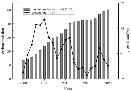
Figure 1.
Total carbon emissions and annual growth rate in China from 2000 to 2020.
The dominant annual consumption of coal increased from 1469 million tons in 2000 to 29.18 million tons in 2006, with an average annual growth rate of 13.26%. The proportion of coal consumption in each province is also in a state of rapid growth, and the added value of national carbon emissions from 2005 to 2008 is 6.48 × 10⁸ tC. The annual growth rate declined rapidly during this period, as it did in the period from 2011 to 2015. It is worth noting that carbon emissions reached negative growth by 2015. Compared with 2014, it decreased by 3.33 × 10⁷ tC. From 2008 to 2011, the growth rate of CO2 emissions gradually picked up, but it was still in a slow growth stage. This may be due to several environmental laws and regulations successively issued in China in recent years, as well as the energy structure adjustment strategy implemented by the provinces.
3.2. Dynamic Evolution Characteristics of Carbon Dioxide Emissions in China
In this paper, to investigate the different concentrations of carbon emissions in different areas and cities over time, non-parametric kernel density estimation with Gaussian ordinary distribution was utilized to assess the kernel density at five observation points (2000, 2005, 2010, 2015, and 2020) and obtain the dispersion at distinctive time points (Figure 2). The height of the curve reflects the degree of concentration of carbon outflows in each area. As can be seen from Figure 2, China’s carbon outflows have a “twofold top” advancement distribution from left to right and from high to low, showing that China’s carbon dioxide outflows increment consistently over time. Early in 2000, the carbon emissions of most territories and cities were at low concentration levels, and the energy consumption expanded amid the “11th five-year plan” as industry expanded. Carbon outflows of all territories and cities appeared to increase to widely differing degrees, but there were still contrasts between total assets and financial quality among areas. The total carbon emissions of all territories and cities started to increase, shaping numerous crests of distinctive adequacy. Be that as it may, the crests of low-level concentration continuously diminished, and by 2015, the gap of the top tallness of bimodal distribution was limited. It is encouraging that that the gap between center- and low-level carbon outflows and high-level carbon emissions appears to be narrowing, demonstrating that territorial contrasts are diminishing. In addition, the kernel density curve showed a right trailing phenomenon, indicating that provinces have relatively high carbon emission levels throughout the country. In some years, the kernel density curve appeared as a “main peak + right peak.” The number of areas with generally high carbon outflow levels expanded, and the gap between territories with a rapid increment in carbon outflow level and territories with a moderate increment in carbon emission level broadened.
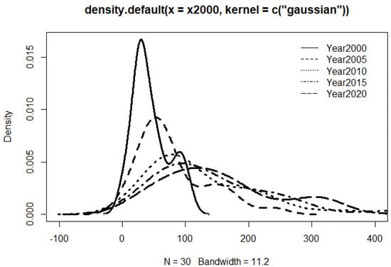
Figure 2.
Kernel density estimation of carbon dioxide emissions in China.
3.3. Spatial Evolution Characteristics of China’s Carbon Emissions
3.3.1. Traditional Markov Probability Transition Matrix
In order to analyze the spatiotemporal advancement characteristics of common carbon emissions in China, the conventional Markov likelihood transfer matrix and spatial-based Markov transfer likelihood matrix were developed. The entire carbon emission was divided into four states: light, common, overwhelming, and super-overwhelming, which are represented by L = 1.2.3.4. Among them, the exchange from low value to high value was characterized as an upward exchange, and the exchange from high value to low value was characterized as a descending exchange. Table 3 shows the conventional Markov exchange likelihood matrix of China’s common carbon emission types from 2000 to 2020, which can be obtained by considering the calculation results: (1) The likelihood values of the inclining lines were all bigger than the likelihood values of the non-diagonal lines, showing that the exchange of types of China’s neighborhood carbon outflow is steady and features a high likelihood of keeping up the first state. (2) There is a phenomenon of “club joining” in common carbon outflows in China, and the likelihood of light and super-overwhelming carbon emissions keeping up the first state within another range is the most elevated, accounting for 89.10% and 99.3%, respectively. (3) The probability of realizing “leapfrog” development of provincial carbon emission type transfer in adjacent years is small, and the probability of realizing trans-grade transfer for each state type is less than 15%.
Table 3.
Traditional Markov probability transfer matrix of China’s carbon emissions from 2000 to 2020.
3.3.2. Spatial Markov Probability Transition Matrix
The spatial Markov transfer probability matrix was constructed by adding spatial lag conditions into the traditional Markov chain transfer probability matrix. The influence of neighborhood background on provincial carbon emission transfer was discussed by comparing and analyzing the transfer probability of provincial carbon emission types under different neighborhood backgrounds.
Table 4 shows the spatial Markov exchange likelihood matrix of carbon outflow types of territories and cities in China from 2000 to 2020. Considering the calculated results, the following can be concluded: (1) Geographical background plays a vital role in the process of carbon emission transfer of provinces in China. Compared with the traditional Markov transition probability matrix, China’s transfer probability of carbon emission types has changed significantly. (2) The carbon emission types of provinces are synergistic with regional carbon emission types. When the neighborhood type is two, the number of provinces and cities with the medium carbon emissions is significantly more than that of other types in the t period; when the neighborhood type is four, the number of provinces and cities with super-heavy carbon emissions is also significantly more than that of other types in t period. (3) By and large, the likelihood of the upward exchange of the carbon emission type of a city will increment when it adjoins a locale with a high carbon outflow level. Figure 3 shows the geographical visualization of carbon emissions in China’s provinces and cities every five years for the past 21 years, It is not difficult to see that it also confirms the above conclusions.
Table 4.
Spatial Markov probability transfer matrix of China’s carbon emissions from 2000 to 2020.
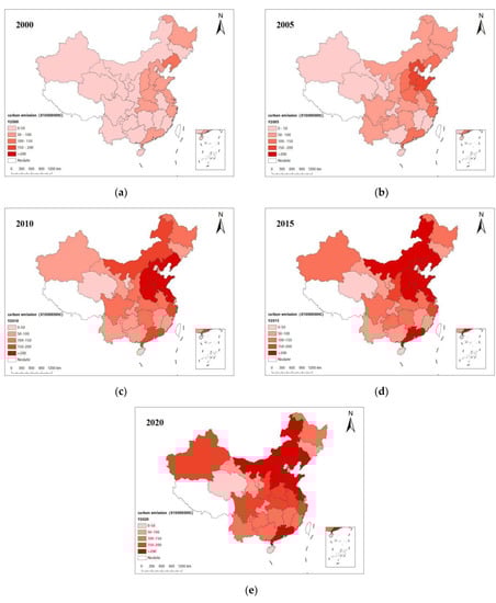
Figure 3.
Temporal and spatial dynamics of carbon emissions by province in China from 2000 to 2020. Among them, (a) represents the spatial distribution pattern of China’s carbon emissions in 2000, (b) represents the spatial distribution pattern of China’s carbon emissions in 2005, (c) represents the spatial distribution pattern of China’s carbon emissions in 2010. (d) represents the spatial distribution pattern of China’s carbon emissions in 2015. (e) represents the spatial distribution pattern of China’s carbon emissions in 2020.
3.4. China’s Carbon Emission Reduction Path
3.4.1. Analysis of Carbon Emission Reduction Potential Index of Provinces
The super-SBM model was used to solve the carbon emission efficiency, and regional carbon emission equity was measured by per capita carbon emission. In order to comprehensively and decently portray the inner flow of territorial carbon emission value and carbon outflow productivity in China, each province’s carbon emission potential index can be calculated by substituting the equity and efficiency weights of each province into Equation (5). This paper presents the carbon emission potential index results for 2000 and 2020, and the specific results are shown in Table 5.
Table 5.
Calculation of carbon emission reduction potential index of provinces in China from the perspective of coordination of carbon emission equity and efficiency.
As seen in Table 5, more than half of the provinces in China had a relatively high emission reduction potential by 2020. The carbon emission reduction potential index of Shanxi, Inner Mongolia, Ningxia, and Xinjiang exceeded 0.8, ranking in the forefront of the country, with a massive responsibility for emission reduction. Moreover, more than two thirds of the provinces in China have reduced their emission reduction potential compared with 2000, and the reduction was quite different. It indicated that most provinces had reached or will reach the peak; less than one third of provinces have improved their emission reduction potential, but the increase was slight, indicating that the emission reduction potential was relatively stable. On the other hand, from the perspective of equity and efficiency coordination, provinces with improved carbon emission reduction potential (i.e., positive difference) meant that their carbon emission reduction potential was mainly driven by carbon emission efficiency and conversely by carbon equity. Therefore, the emission reduction of most provinces in China should focus on improving the efficiency of carbon emissions. Provinces such as Inner Mongolia, Fujian, Ningxia, and Xinjiang should focus on improving carbon emission efficiency to reduce carbon emissions.
3.4.2. Carbon Emission Reduction Path
In order to further investigate more compelling ways to diminish emissions, this paper built a two-dimensional matrix scatter plot based on carbon outflow proficiency and normal per capita carbon emission levels and partitioned the carbon outflow lessening circumstance of different areas in China into districts. As the two-dimensional matrix of the scatter plot shown in Figure 4, the abscissa represents “carbon emission efficiency,” the ordinate represents “carbon emission equity (per capita carbon emission),” and the two dotted lines represent the overall median level of carbon emission per capita and carbon emission efficiency, respectively. Therefore, the 30 provincial administrative regions in mainland China can be divided into four regions: “low efficiency and low emission” type (from now on referred to as Region A), “high efficiency and low discharge” type (from now on referred to as Zone B); “high efficiency and high discharge” type (from now on referred to as Zone C); “low efficiency and high discharge” type (from now on referred to as Region D).
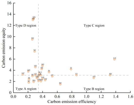
Figure 4.
“Equity-efficiency” path matrix of carbon emission reduction. In the picture, we use BJ to represent Beijing, and so on for the other cities.
Under the current carbon emission efficiency, the more carbon emission permits, the more space for economic development, the more beneficial to regional economic development, that is to say, the reduction of carbon emission permits is bound to limit economic development. Therefore, how to better allocate carbon rights has become a focus issue, which can also be understood as how to find a more effective carbon emission reduction path. For any region, how to accomplish regional carbon emission reduction tasks can be considered from two perspectives—improving carbon emission efficiency and reducing carbon emission rights (equity). These two perspectives can also be regarded as two types of resources so that the problem of carbon emission reduction can be transformed into a problem of allocating these two types of resources. Through analysis, this paper believes that the task focus of regional carbon emission reduction should be placed in region A; that is, region A should be taken care of. The government should increase the allocation of category I resources (the carbon emission efficiency) in Region A, such as increasing the support of environmental protection technology and new energy technology, to improve the carbon emission efficiency in Region A and achieve carbon emission reduction. This makes region A enter Region B, that is, realize the carbon emission reduction path from A to B.
Above all, the government should prioritize supporting Region A and improving the carbon emission efficiency of provinces in Region A (such as Sichuan, Jiangxi, Anhui, Henan, etc.). It can reduce carbon emissions from the viewpoint of focusing on efficiency, alleviate the current regional carbon emission efficiency and equity disharmony, and achieve dynamic coordination between efficiency and equity. In addition, for local governments, since significant differences in regional emissions determined the complexity of emission reduction paths, local governments can adopt flexible carbon emission reduction paths according to their conditions. As shown in Figure 4, the “low-efficiency and high-discharge” category D regions include Shanxi, Xinjiang, and Qinghai provinces, which are “low-efficiency and high-discharge” provinces due to backward production level, and Inner Mongolia, Shanxi and Ningxia provinces, which are “low-efficiency and high-discharge” provinces due to extensive utilization of resources. In addition to the “incentive path” of D→A→B, D→C→B can also be considered for “low-efficiency and medium discharge” provinces, which may be more feasible.
4. Conclusions and Policy Recommendation
4.1. Conclusions
It is of awesome importance to think about the advancement of the spatiotemporal design of carbon emissions and the outflow lessening method for directing carbon emission decrease. This paper embraces the IPCC outflows calculation model and generation of cement carbon emissions calculation model for the assurance of the whole carbon outflow of the territories. The spatial spillover impact of the amount of China’s urban carbon emissions is experimentally analyzed by developing conventional and spatial Markov chain exchange likelihood matrices, and the spatiotemporal energetic advancement characteristics of the amount of urban carbon emissions are determined. At the same time, utilizing the super-SBM model, counting the non-expected yield to calculate the carbon emission productivity of 30 territories in China from 2000 to 2020, this study measured territorial carbon emissions values based on per capita carbon emissions, calculated the emissions lessening potential of each area and strategy, and gives a logical basis for the government to define carbon emission diminishment measures. The particular research conclusions were as follows:
- In terms of the distribution of spatiotemporal patterns, the total carbon emissions of our provinces are rising steadily. The change in the total growth rate of carbon emissions in each province and city developed from high concentration to diffuse and median concentration distribution patterns. The total carbon emissions gradually spread outward, mainly in the Beijing–Tianjin–Hebei and Liaoning regions with high energy consumption as the core;
- From the point of view of the characteristics of time and space advancement, there is a phenomenon of “club joining” in carbon emissions from all territories and cities in China. It is not simple to attain “leapfrog” advancement in adjoining a long time. Beneath a distinctive topographical foundation, the likelihood of carbon outflow exchange in Chinese cities has essentially changed. When cities are adjoining to regions with higher total carbon outflows, the likelihood of an upward move in carbon outflows type increments. Due to the spillover impact of the neighborhood type, carbon outflows from different areas and cities in China show “club merging” tendencies inside particular geospaces;
- Based on the different characteristics of carbon emission equity and efficiency in each province, China’s provinces and regions can be divided into four categories: “high efficiency and high emission,” “low efficiency and low emission,” “high efficiency and low emission” and “low efficiency and high emission.” The carbon outflow lessening strategy proposes that areas that center on supporting “wasteful, low-emission” zones ought to be backed to progress carbon emission productivity in these regions and to realize energetic coordination of carbon emission value and proficiency.
4.2. Policy Suggestions
Based on the experimental conclusions, this paper puts forward some recommendations for China to decrease carbon outflows and accomplish “double carbon” objectives as follows:
To begin with, due to the characteristics of China’s energy resources, that is, “wealthy in coal, destitute in oil and small in gas,” its financial advancement depends exceedingly on coal with high carbon emissions, and its energy utilization structure is outlandish. In this manner, to attain the objective of “double carbon,” China must essentially diminish coordinate coal utilization (particularly bulk coal utilization), diminish the extent of coal in essential energy utilization. The fundamental solution is to gradually eliminate the high dependence on coal. Specifically, provinces such as Xinjiang, Ningxia, and Qinghai, which have seen the biggest energy consumption, should strictly control total energy consumption by reducing energy intensity. In contrast, areas such as Beijing and Shanghai, which have already experienced huge decreases in carbon emission rates, ought to fittingly unwind the reduction task and center on making strides yield execution. At the same time, power is China’s fundamental source of carbon emissions, and warm control accounts for the most elevated extent. In this manner, on the energy supply side, the whole scale of coal-fired power plants ought to be sensibly controlled to extend the extent of clean energy within the total energy sector. On the consumer side, the government ought to proceed to advance energy substitution ventures in transportation, heating, industry, and development.
Secondly, China ought to continue the advancement of energy innovation, which is the basic driving force for energy change and the key driving constraint and unavoidable choice for realizing the “dual carbon” objective. In this manner, long-standing plans must be backed by progressive and progressed mechanical breakthroughs and development, and the advancement and application of low-carbon innovations must be quickened. Specifically, China’s central and western provinces should introduce advanced clean and energy-saving production technologies from developed and eastern countries. At the same time, the Beijing–Tianjin–Hebei region and the southeastern coastal region should focus on developing carbon capture, utilization, and storage (CCUS) technology, strengthening R&D on energy storage and smart grid technology and expanding the scale of demonstrations. At the same time, territories also ought to speed up the arrangement of modern energy passenger and hydrogen fuel cell vehicles, consider carbon dioxide emission lessening advances in key businesses, and define a comprehensive greenhouse gas control innovation plan.
Finally, the advancement of renewable energy may be a key way to accomplishing energy alter and an imperative way to bargain with climate alter and diminish greenhouse gas emissions. China ought to proceed to effectively advance the development of renewable energy in order to realize the genuine energy transition and “double carbon” emission lessening targets. Specifically, the provinces should accelerate the implementation of renewable energy replacement actions in the power industry, and the eastern, central, and southern regions should promote the nearby development of wind and photovoltaic power. The “three North regions” should further accelerate the development of wind power and photovoltaic bases and accelerate the promotion of renewable energy generation technology. Coastal coal-consuming provinces such as Liaoning, Hebei, and Shandong should actively promote the development of offshore wind power clusters, focusing on the construction of clean energy utilization demonstration zones.
Author Contributions
Conceptualization, F.Q.; Data curation, W.S. and Z.S.; Formal analysis, W.S. and Z.S.; Investigation, C.L.; Methodology, W.T.; Visualization, Y.Z. and C.W.; Writing—review and editing, J.G. All authors have read and agreed to the published version of the manuscript.
Funding
This research was funded by the Gansu Provincial Natural Science Foundation, China (grant no. 22JR5RA155) and Key Laboratory of Resource Environment and Sustainable Development of Oasis, Gansu Province; Higher Education Innovation Fund Projects in Gansu Province, grant number 2021B–087, and Project of Improving Young Teachers’ Scientific Research Ability in Northwest Normal University, grant number NWNU–SKQN2021–22.
Institutional Review Board Statement
Not applicable.
Informed Consent Statement
Not applicable.
Data Availability Statement
Not applicable.
Conflicts of Interest
The authors declare no conflict of interest.
References
- Song, Y.; Huang, J.-B.; Feng, C. Decomposition of energy-related CO2 emissions in China’s iron and steel industry: A comprehensive decomposition framework. Resour. Policy 2018, 59, 103–116. [Google Scholar] [CrossRef]
- Hao, Y.; Chen, H.; Wei, Y.-M.; Li, Y.-M. The influence of climate change on CO 2 (carbon dioxide) emissions: An empirical estimation based on Chinese provincial panel data. J. Clean. Prod. 2016, 131, 667–677. [Google Scholar] [CrossRef]
- Li, B.; Gasser, T.; Ciais, P.; Piao, S.; Tao, S.; Balkanski, Y.; Hauglustaine, D.; Boisier, J.-P.; Chen, Z.; Huang, M.; et al. The contribution of China’s emissions to global climate forcing. Nature 2016, 531, 357–361. [Google Scholar] [CrossRef]
- Liu, Z.; Guan, D.; Crawford-Brown, D.; Zhang, Q.; He, K.; Liu, J. A low-carbon road map for China. Nature 2013, 500, 143–145. [Google Scholar] [CrossRef]
- Li, K.; Lin, B. Economic growth model, structural transformation, and green productivity in China. Appl. Energy 2017, 187, 489–500. [Google Scholar] [CrossRef]
- Lai, L.; Huang, X.; Yang, H.; Chuai, X.; Zhang, M.; Zhong, T.; Chen, Z.; Chen, Y.; Wang, X.; Thompson, J.R. Carbon emissions from land-use change and management in China between 1990 and 2010. Sci. Adv. 2016, 2, e1601063. [Google Scholar] [CrossRef] [PubMed]
- Zhang, W.; Li, K.; Zhou, D.; Zhang, W.; Gao, H. Decomposition of intensity of energy-related CO2 emission in Chinese provinces using the LMDI method. Energy Policy 2016, 92, 369–381. [Google Scholar] [CrossRef]
- Su, B.; Ang, B. Structural decomposition analysis applied to energy and emissions: Some methodological developments. Energy Econ. 2012, 34, 177–188. [Google Scholar] [CrossRef]
- Ang, B.; Su, B. Carbon emission intensity in electricity production: A global analysis. Energy Policy 2016, 94, 56–63. [Google Scholar] [CrossRef]
- Radonjič, G.; Tompa, S. Carbon footprint calculation in telecommunications companies–The importance and relevance of scope 3 greenhouse gases emissions. Renew. Sustain. Energy Rev. 2018, 98, 361–375. [Google Scholar] [CrossRef]
- Kai, W.; Xiaohui, T.; Chang, G.; Haolong, L. Temporal-spatial evolution and influencing factors of carbon emission intensity of China’s service industry. China Popul. Resour. Environ. 2021, 31, 23–31. [Google Scholar] [CrossRef]
- Gallo, M.; Del Borghi, A.; Strazza, C. Analysis of potential GHG emissions reductions from methane recovery in livestock farming. Int. J. Glob. Warm. 2015, 8, 516–533. [Google Scholar] [CrossRef]
- Si, Y.; Yuan, Z.; Xin, X.; Qi, W.; Pan, P.; Wen, M. Regional differences, temporal and spatial patterns and dynamic evolution of China’s agricultural carbon emission intensity in the past 20 years Resour. Environ. Yangtze Basin 2020, 29, 596–608. [Google Scholar] [CrossRef]
- Liu, H.; Song, Y. Financial development and carbon emissions in China since the recent world financial crisis: Evidence from a spatial-temporal analysis and a spatial Durbin model. Sci. Total. Environ. 2020, 715, 136771. [Google Scholar] [CrossRef]
- Wang, Y.; Yang, H.; Sun, R. Effectiveness of China’s provincial industrial carbon emission reduction and optimization of carbon emission reduction paths in "lagging regions": Efficiency-cost analysis-ScienceDirect. J. Environ. Manag. 2020, 275, 111221. [Google Scholar] [CrossRef] [PubMed]
- Peng, S.; Zhang, W.; Sun, C. China’s Production-Based and Consumption-Based Carbon Emissions and Their Determinants. Econ. Res. J. 2015, 50, 168–182, (In Chinese with English Summary). [Google Scholar]
- Yuquan, Z.; Huang, Y.; Wang, S. Spatial spillover effect and driving forces of carbon emission intensity at the city level in China. J. Geogr. Sci. 2019, 74, 231–252. [Google Scholar] [CrossRef]
- Song, G.; Wang, Y.; Jiang, Y. Carbon emission control policy design based on the targets of carbon peak and carbon neutrality. China Popul. Resour. Environ. 2021, 31, 55–63. [Google Scholar] [CrossRef]
- Schipper, L.; Murtishaw, S.; Khrushch, M.; Ting, M.; Karbuz, S.; Unander, F. Carbon emissions from manufacturing energy use in 13 IEA countries: Long-term trends through 1995. Energy Policy 2001, 29, 667–688. [Google Scholar] [CrossRef]
- Casler, S.D.; Rose, A. Carbon Dioxide Emissions in the U.S. Economy: A Structural Decomposition Analysis. Environ. Resour. Econ. 1998, 11, 349–363. [Google Scholar] [CrossRef]
- Zhao, F.; Yao, Y. Analysis on space-time difference and influencing factors of carbon emission efficiency in Hunan Province based on SBM-DEA model. Sci. Geogr. Sin. 2019, 39, 797–806. [Google Scholar] [CrossRef]
- Wang, S.; Fang, C.; Wang, Y. Spatiotemporal variations of energy-related CO 2 emissions in China and its influencing factors: An empirical analysis based on provincial panel data. Renew. Sustain. Energy Rev. 2016, 55, 505–515. [Google Scholar] [CrossRef]
- Yang, W.Y.; Cao, X.S. The influence mechanism of travel-related CO2 emissions from the perspective of residential self-selection: A case study of Guangzhou. Acta Geogr. Sin. 2018, 73, 346–361. [Google Scholar] [CrossRef]
- Ming, G.; Hong, Y. Spatial Convergence and Differentiation of China’s Agricultural Carbon Emission Performance: An Empirical Analysis Based on Malmquist luenberger Index and Spatial Measurement. Econ. Geogr. 2015, 35, 142–148, 185. [Google Scholar] [CrossRef]
- Han, M.; Yao, Q.; Lao, J.; Tang, Z.; Liu, W. China’s intra- and inter-national carbon emission transfers by province: A nested network perspective. Sci. China Earth Sci. 2020, 63, 852–864. [Google Scholar] [CrossRef]
- Xiao, G.; Yao, H. Influence factors and Environmental Kuznets Curve relink effect of Chinese industry’s carbon dioxide emission: Eempirical research based on STIRPAT model with industrial dynamic panel data. China Ind. Econ. 2012, 1, 26–35. [Google Scholar] [CrossRef]
- Zhipeng, T.; Weidong, L. Peiping, G. Measuring of Chinese regional carbon emission spatial effects induced by exports based on Chinese multi-regional input-output table during 1997–2007. Acta Geogr. Sin. 2014, 69, 1403–1413. [Google Scholar] [CrossRef]
- Wang, S.; Fang, C.; Wang, Y. Review of energy- related CO2 emission in response to climate change. Prog. Geogr. 2015, 34, 151–164. [Google Scholar] [CrossRef]
- Liu, S.; Xiao, Q. An empirical analysis on spatial correlation investigation of industrial carbon emissions using SNA-ICE model. Energy 2021, 224, 120183. [Google Scholar] [CrossRef]
- Wang, B.; Yu, M.; Zhu, Y.; Bao, P. Unveiling the driving factors of carbon emissions from industrial resource allocation in China: A spatial econometric perspective. Energy Policy 2021, 158, 112557. [Google Scholar] [CrossRef]
- Lu, H.; Liu, G. Spatial effects of carbon dioxide emissions from residential energy consumption: A county-level study using enhanced nocturnal lighting. Appl. Energy 2014, 131, 297–306. [Google Scholar] [CrossRef]
- Rong, P.; Zhang, Y.; Qin, Y.; Liu, G.; Liu, R. Spatial differentiation of carbon emissions from residential energy consumption: A case study in Kaifeng, China-ScienceDirect. J. Environ. Manag. 2020, 271, 110895. [Google Scholar] [CrossRef] [PubMed]
- Yue, J.; Zhu, H.; Yao, F. Does Industrial Transfer Change the Spatial Structure of CO2 Emissions?—Evidence from Beijing-Tianjin-Hebei Region in China. Int. J. Environ. Res. Public Health 2021, 19, 322. [Google Scholar] [CrossRef] [PubMed]
- Heil, M.T.; Wodon, Q.T. Inequality in CO2 Emissions Between Poor and Rich Countries. J. Environ. Dev. 1997, 6, 426–452. [Google Scholar] [CrossRef]
- Guo, Q.; Zhu, C.; Shi, W. A Study on the Temporal and Spatial Differences of Carbon Emissions and Their Influencing Factors Based on the Two stage LMDI Model—A Case Study of Jiangsu Province. Soft Sci. 2021, 35, 107–113. [Google Scholar] [CrossRef]
- Cheng, Y.; Wang, Z.; Ye, X.; Wei, Y.D. Spatiotemporal dynamics of carbon intensity from energy consumption in China. J. Geogr. Sci. 2014, 24, 631–650. [Google Scholar] [CrossRef]
- Mirza, F.M.; Kanwal, A. Energy consumption, carbon emissions and economic growth in Pakistan: Dynamic causality analysis. Renew. Sustain. Energy Rev. 2017, 72, 1233–1240. [Google Scholar] [CrossRef]
- Shi, K.; Yu, B.; Zhou, Y.; Chen, Y.; Yang, C.; Chen, Z.; Wu, J. Spatiotemporal variations of CO2 emissions and their impact factors in China: A comparative analysis between the provincial and prefectural levels. Appl. Energy 2019, 233–234, 170–181. [Google Scholar] [CrossRef]
- Wang, Y.; He, X. Spatial economic dependency in the Environmental Kuznets Curve of carbon dioxide: The case of China. J. Clean. Prod. 2019, 218, 498–510. [Google Scholar] [CrossRef]
- Kai, W.; Shu, W.; Chang, G.; Ya, P.; Hao, L. Spatial correlation of carbon emissions from tourism in China and its impact factors. Sci. Geogr. Sin. 2019, 32, 938–947. [Google Scholar] [CrossRef]
- Guan, Y.; Kang, L.; Shao, C.; Wang, P.; Ju, M. Measuring county-level heterogeneity of CO2 emissions attributed to energy consumption: A case study in Ningxia Hui Autonomous Region, China. J. Clean. Prod. 2017, 142, 3471–3481. [Google Scholar] [CrossRef]
- Cai, B.; Zhang, L. Urban CO2 emissions in China: Spatial boundary and performance comparison. Energy Policy 2014, 66, 557–567. [Google Scholar] [CrossRef]
- Zhe, X.; Qin, Z.R. Impacts of Population Dynamics and Consumption Pattern on Carbon Emission in China. Popul. Res. 2010, 34, 48–58. [Google Scholar]
- Huang, J.; Fang, C. Analysis of coupling mechanism and rules between urbanization and eco-environment. Geogr. Res. 2003. [CrossRef]
- Chao, J.; Hong, O.; Ye, Y.; Yong, X.; Lian, W. Analysis on the Impact Mechanism of Energy Consumption and Carbon Emission in Guangdong Province-Based on IO-SDA Model. Trop. Geogr. 2017, 37, 10–18. [Google Scholar] [CrossRef]
- Nguyen, D.K.; Huynh, T.L.D.; Nasir, M.A. Carbon emissions determinants and forecasting: Evidence from G6 countries. J. Environ. Manag. 2021, 285, 111988. [Google Scholar] [CrossRef]
- Alam, M.J.; Begum, I.A.; Buysse, J.; Van Huylenbroeck, G. Energy consumption, carbon emissions and economic growth nexus in Bangladesh: Cointegration and dynamic causality analysis. Energy Policy 2012, 45, 217–225. [Google Scholar] [CrossRef]
- Padilla, E.; Serrano, A. Inequality in CO2 emissions across countries and its relationship with income inequality: A distributive approach. Energy Policy 2006, 34, 1762–1772. [Google Scholar] [CrossRef]
- Zhou, K.; Yang, J.; Yang, T.; Ding, T. Spatial and temporal evolution characteristics and spillover effects of China’s regional carbon emissions. J. Environ. Manag. 2023, 325, 116423. [Google Scholar] [CrossRef] [PubMed]
- Chen, J.; Dong, X. Carbon efficiency and carbon abatement costs of coal-fired power enterprises: A case of Shanghai, China. J. Clean. Prod. 2019, 206, 452–459. [Google Scholar] [CrossRef]
- Zhu, B.; Jiang, M.; Wang, K.; Chevallier, J.; Wang, P.; Wei, Y.-M. On the road to China’s 2020 carbon intensity target from the perspective of “double control”. Energy Policy 2018, 119, 377–387. [Google Scholar] [CrossRef]
- Zhang, Y.; Liu, C.; Chen, L.; Wang, X.; Song, X.; Li, K. Energy-related CO2 emission peaking target and pathways for China’s city: A case study of Baoding City. J. Clean. Prod. 2019, 226, 471–481. [Google Scholar] [CrossRef]
- Fang, K.; Tang, Y.; Zhang, Q.; Song, J.; Wen, Q.; Sun, H.; Ji, C.; Xu, A. Will China peak its energy-related carbon emissions by 2030? Lessons from 30 Chinese provinces. Appl. Energy 2019, 255, 113852. [Google Scholar] [CrossRef]
- Ma, H.; Sun, W.; Wang, S.; Kang, L. Structural contribution and scenario simulation of highway passenger transit carbon emissions in the Beijing-Tianjin-Hebei metropolitan region, China. Resour. Conserv. Recycl. 2018, 140, 209–215. [Google Scholar] [CrossRef]
- Wang, D.; He, W.; Shi, R. How to achieve the dual-control targets of China’s CO2 emission reduction in 2030? Future trends and prospective decomposition. J. Clean. Prod. 2018, 213, 1251–1263. [Google Scholar] [CrossRef]
- Paustian, K.; Ravindranath, N.H.; van Amstel, A.R. 2006 IPCC Guidelines for National Greenhouse Gas Inventories; IPCC: Geneva, Switzerland, 2006. [Google Scholar]


Disclaimer/Publisher’s Note: The statements, opinions and data contained in all publications are solely those of the individual author(s) and contributor(s) and not of MDPI and/or the editor(s). MDPI and/or the editor(s) disclaim responsibility for any injury to people or property resulting from any ideas, methods, instructions or products referred to in the content. |
© 2023 by the authors. Licensee MDPI, Basel, Switzerland. This article is an open access article distributed under the terms and conditions of the Creative Commons Attribution (CC BY) license (https://creativecommons.org/licenses/by/4.0/).