Overview of Common Thermophysical Property Modelling Approaches for Cryogenic Fluid Simulations at Supercritical Conditions

Abstract

Computational Fluid Dynamics (CFD) frameworks of supercritical cryogenic fluids need to employ Real Fluid models such as cubic Equations of State (EoS) to account for thermal and inertial driven mechanisms of fluid evolution and disintegration. Accurate estimation of the non-linear variation in density, thermodynamic and transport properties is required to computationally replicate the relevant thermo and fluid dynamics involved. This article reviews the availability, performance and the implementation of common Real Fluid EoS and data-based models in CFD studies of supercritical cryogenic fluids. A systematic analysis of supercritical cryogenic fluid (N₂, O₂ and CH₄) thermophysical property predictions by cubic (PR and SRK) and non-cubic (SBWR) Real Fluid EoS, along with Chung’s model, reveal that: (a) SRK EoS is much more accurate than PR at low temperatures of liquid phase, whereas PR is more accurate at the pseudoboiling region and (b) SBWR EoS is more accurate than PR and SRK despite requiring the same input parameters; however, it is limited by the complexity in thermodynamic property estimation. Alternative data-based models, such as tabulation and polynomial methods, have also been shown to be reliably employed in CFD. At the end, a brief discussion on the thermophysical modelling of cryogenic fluids affected by quantum effects is included, in which the unsuitability of the common real fluid EoS models for the liquid phase of such fluids is presented.

1. Introduction

Cryogenic fluids are gases in atmospheric conditions which transition to liquid phase usually below 120 K. Common cryogenic fluids include liquid nitrogen (LN${}_2$), liquid oxygen (LO${}_X$), liquified natural gas (LNG), liquid air, liquid helium (LHe) and liquid hydrogen (LH${}_2$). At present, cryogenic fluids are used in a range of application including MRI (Magnetic Resonance Imaging), NMR (Nuclear Magnetic Resonance), cryogenic rocket engines, LTS (low temperature superconductors) [1] as well as in propulsion systems such as the case of high efficiency Internal Combustion Engines-Cryopower RSCE [2,3,4] and `methalox’ cryogenic rocket engines [5,6].

Cryogenic fluids exist as liquids at very low temperatures even at atmospheric pressures, although in practice their transportation and storage requires compression at high pressures as well. When they are used in a real life applications they will transition from their liquid state that are maintained during storage back to their natural gaseous state after being exposed to a high pressure and temperature operating environment. Here we refer as “high” operating conditions above their critical point (see Table 1) which results in complex phase change phenomena taking place. For instance, in cryogenic rocket engines while the fuel (liquid hydrogen) and oxidiser (liquid oxygen) are stored in their liquid phase at low temperatures and high pressures, the prevailing environment inside the combustion chamber that they are injected is approximately 10 to 15 MPa and 3000 K which is a supercritical environment for both hydrogen and oxygen. The same is the case of methane that is used as fuel in methalox cryogenic rocket engines. Another example is the compression chamber of Cryopower RSCE Internal Combustion Engine, where liquid nitrogen is utilised as a coolant in the compression chamber [2,4]. The maximum pressure in the chamber can reach up to 7 MPa and the temperature exceeds 300 K, which is again supercritical for nitrogen.

At subcritical pressures, the cryogenic liquids behave similarly to atmospheric liquids. When injected into high temperature environments, they break into droplets and ligaments before vaporisation [7,8]. In our previous work we have shown that cryogenic fluids obey primary atomisation/breakup regimes traditionally utilised for the categorisation of atmospheric liquids [4]. On the contrary, at supercritical pressures, the injected cryogenic liquid diffuses into the ambient environment more like a turbulent gas jet without exhibiting the traditional primary and secondary breakup characteristics. This unique behaviour of cryogenic liquids injected into supercritical environment has been extensively experimented and examined by Mayer et al. [7,9,10,11,12], Oschwald et al. [13,14,15] and Chehroudi et al. [8,16,17].

Table 1. Table of respective fluid critical properties of five cryogenic fluids (N${}_2$, O${}_2$, H${}_2$, He and CH${}_4$). Data obtained from NIST webbook database [18].

Fluid	Critical	Critical
	Pressure	Temperature
	${\mathit{P}}_{\mathit{c}}$ (MPa)	${\mathit{T}}_{\mathit{c}}$ (K)
Nitrogen-N${}_2$	3.3958	126.192
Oxygen-O${}_2$	5.0430	154.581
Methane-CH${}_4$	4.5992	190.564
Hydrogen-H${}_2$	1.2964	33.145
Helium-He	0.22832	5.1953

Table 1. Table of respective fluid critical properties of five cryogenic fluids (N${}_2$, O${}_2$, H${}_2$, He and CH${}_4$). Data obtained from NIST webbook database [18].

Fluid	Critical	Critical
	Pressure	Temperature
	${\mathit{P}}_{\mathit{c}}$ (MPa)	${\mathit{T}}_{\mathit{c}}$ (K)
Nitrogen-N${}_2$	3.3958	126.192
Oxygen-O${}_2$	5.0430	154.581
Methane-CH${}_4$	4.5992	190.564
Hydrogen-H${}_2$	1.2964	33.145
Helium-He	0.22832	5.1953

An additional peculiarity of these fluids is that while for liquid sprays and gas jets at atmospheric and subcritical pressures the thermophysical properties of the fluid (both liquid and gas) can be assumed to be constant or having a linear dependency to temperature, at supercritical pressure conditions these assumptions are not valid. The continuous yet non-linear behaviour of cryogenic fluids and the associated thermophysical properties at supercritical pressures around the critical temperature has been discussed for isolated supercritical pressures under consideration by various researchers [10,19,20,21,22,23,24,25] and expanded in a systematic manner for a wider range of supercritical pressures by some of them [4,5]. To elaborate, the steep drop in density and drastic spikes in specific heat capacity of nitrogen around the critical temperature at supercritical pressures of 4 and 6 MPa were presented by Mayer et al. [10], corresponding to his liquid nitrogen injection experiments and later on by Kim et al. [19] for numerical simulation of Mayer et al.’s experiments. However, it is not only the density which undergoes this steep transition, even the viscosity and thermal conductivity of nitrogen were observed to transition steeply at these pressures [21,22,23,24]. In [4,5] the variations of all these properties for a range of supercritical (from low to high supercritical) pressures of nitrogen (4 to 10 MPa) are shown. This non-linearity in the properties and behaviour of the fluids at supercritical conditions is referred to as real fluid behaviour, and is common for all fluids at supercritical pressures around the critical temperature. In the case of most applications of cryogenic fluids where the pressure is supercritical, the large temperature difference between the storage and operating conditions makes them go through the critical temperature while transitioning from injection state towards the operating state, which makes these fluids highly sensitive to the thermal influence in addition to the flow dynamics. In other words, the evolution of such injected cryogenic fluids/jets is controlled by both thermal and inertia phenomena. The thermal influence on the cryogenic jet evolution known as ’thermal disintegration mechanism’ has been first analysed in significant detail by Banuti [26], who focused on the liquid nitrogen injection into supercritical pressure and temperature environment corresponding to the experiments of Mayer et al. [10]. He demonstrated that the decay of such nitrogen jets were strongly influenced by the thermodynamic state (and properties) of the fluid. More recently, in [4,5] the interplay of the thermal and the mechanical disintegration mechanisms (including turbulence) was also investigated.

One of the primary requirements for Computational Fluid Dynamics (CFD) approaches in order to accurately simulate the evolution dynamics of cryogenic fluids at supercritical pressures is the implementation of numerical models that are able to estimate thermodynamic properties—enthalpy/specific heat capacity and thermal conductivity (to account for the thermal interactions), in addition to density and viscosity (to account for inertial and mechanical effects) adequately as they vary with temperature. The National Institute of Standards and Technology (NIST) Reference Fluid Thermodynamic and Transport Properties Database (REFPROP) [27] is considered to be one of the most accurate databases for the thermophysical properties of single-component cryogenic and supercritical fluids. However, it should be noted that the database is in reality built upon several individual models including, but not limited to, Modified Benedict Webb Rubin (MBWR) [28,29], Helmholtz-energy equation of state and Extended Corresponding States (ECS) each having their applicability limitations. Another alternative is the CoolProp [30] built upon Helmholtz-energy equation of state. Although several exclusive Equations of State (EoS) have been specifically developed for natural gas and natural gas mixtures such as Perturbed Chain-Statistical Associating Fluid Theory (PC-SAFT) [31] and Groupe Européen de Recherches Gazières (GERG-2004) [32] and its subsequent expansion to GERG-2008 [33] EoS, none such EoS or thermophysical models exist specifically for cryogenic fluids. While Liquified Natural Gas (LNG) and liquid CH${}_4$, being cryogenic could make use of natural gas/gas-mixture specific EoS mentioned above, Cubic EoS such as Peng–Robinson (PR) [34] and Soave-Redlich-Kwong (SRK) [35] are still the most preferred EoS for non-hydrocarbon single-component and multi-component cryogenic fluid simulations.

One point that needs to be highlighted is that, although there are several more complex real fluid EoS models—than the ones mentioned above–available in the literature, the focus in this paper would be specifically on common EoS which do not require extensive fluid-specific parameters. The reason is that when CFD frameworks are developed they need to be general to model a wide range of fluids and conditions. Implementation of case specific thermophysical models limits the applicability of the numerical approaches although in some case might be beneficial in terms of accuracy. The cubic EoS are a good fit to be coupled with CFD approaches as they only require as input the critical parameters of the fluid under consideration. This enables these EoS to be utilised for several different cryogenic fluids in CFD simulations, without the need to model them according to specific fluids. Although the cubic EoS only relates the state variables from which the density can be obtained directly, the thermodynamic properties can be obtained from the use of departure functions and ideal gas values. However for the prediction of the transport properties-viscosity and thermal conductivity, additional models that provide coupling with the EoS exist. See for example the work presented in a range of publications [36,37,38,39,40]. In this paper the applicability of these EoS and of the supplementary models will be limited to commonly used cryogenic fluids (such as for example N${}_2$). Hydrogen and helium are excluded because quantum effects come in to play. Only a brief discussion will be included in the end of the paper for completeness.

The paper is structured as follows: After introducing (above) the need for real fluid thermophysical/EoS models in CFD simulations of cryogenic fluids at supercritical pressure environments, a brief overview of the variation in thermophysical properties from cryogenic temperatures to high temperatures at supercritical pressures of nitrogen (N${}_2$) is presented using NIST data [18]. This introductory analysis of N${}_2$ is included in order to provide a better understanding of the drastic yet continuous variation around the temperatures of phase transition at supercritical pressures. Then, starting with a review of the real fluid EoS commonly utilised in numerical simulations, specific cubic and non-cubic EoS (PR, SRK and SBWR) are discussed. This is also followed by a brief demonstration of how to obtain thermodynamic and transport properties from these EoS. The performance of these EoS models in the estimation of the thermophysical properties of cryogenic N${}_2$, O${}_2$, and CH${}_4$ at supercritical pressures are presented and compared against NIST data. This is then followed by a review of past CFD approaches and the real fluid EoS utilised in them to simulate cryogenic fluids introduced into supercritical pressure environments. For completeness, alternative data based thermophysical models-polynomial fitting of NIST data and tabulated thermophysical properties- used in some numerical simulation studies to mitigate the complexities in using real fluid EoS are also discussed. Lastly, the peculiarities associated with modelling cryogenic fluids influenced by quantum effects are discussed briefly along with the deficiencies of utilising common real fluid EoS for such fluids. Finally, the important conclusions summarise the current state of common real fluid EoS and other thermophysical models used in CFD simulations of cryogenic fluids in supercritical environments.

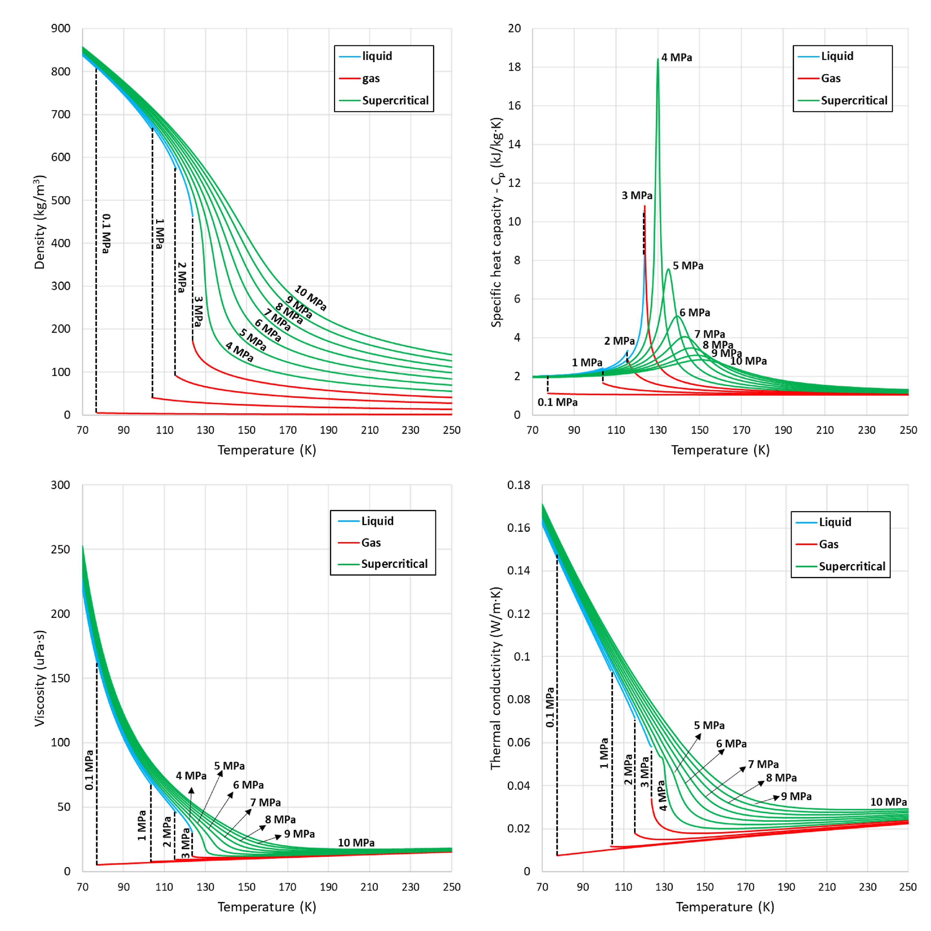
2. Peculiarities of Thermophysical Properties at Supercritical Pressure Conditions

To understand the thermophysical transition of cryogenic fluids at supercritical conditions, the NIST isobaric thermophysical properties (density, specific heat capacity at constant pressure, viscosity and thermal conductivity) of N${}_2$ chosen as the case fluid are presented for various pressures, starting from a low subcritical pressure of 0.1 MPa and up to a high supercritical pressure of 10 MPa (see Figure 1 adapted from [4]). The reason that N${}_2$ is chosen is because it is well studied and experimented due to its inertness, abundance, cost and safety, and furthermore LN${}_2$ has been often used as surrogate for other cryogenic fluids in experiments [7,9,10]. The plots presented here for a series of 10 isobaric pressures (from low subcritical to high supercritical) shed light on the thermophysical property variation with increase/decrease in pressures as well as the isobaric conditions that are representative of many of its applications.

From the plots in Figure 1, it can be seen that at subcritical pressures from a very low temperature of 70 K with increase in temperature the LN${}_2$ eventually reaches the boiling temperature where phase transition from liquid to gas takes place. The thermophysical properties instantly change from that of a liquid to that of a gas. In the figure, the phase change corresponding to the discontinuity in the thermophysical properties at subcritical pressures of 0.1 MPa to 3 MPa is denoted by dashed lines. Above the boiling point, for subcritical pressures the gas phase density, specific heat capacity, viscosity, and thermal conductivity can be assumed constant or linear. While at near-critical subcritical pressures ($P_c$ = 3.396 MPa for N${}_2$) gradients start to appear near the boiling temperature, the boiling point discontinuity still persists. Whereas above the critical pressure the discontinuity ceases and the transition from liquid to supercritical fluid occurs without any associated thermophysical property discontinuity.

Although beyond the critical point the fluid is generally known as a supercritical fluid, with increase in temperature at supercritical pressures, around the critical temperature the thermophysical properties-density, viscosity and thermal conductivity, transform from properties of liquid to that of something like a gas phase as in the case of N${}_2$ from the figure. The difference to subcritical pressures is that the phase change occurs in a continuous manner over a temperature range. In terms of heat capacity, as the temperature of the fluid approaches this temperature, there is a distinct rise in isobaric specific heat capacity which peaks at a particular temperature before falling back, and this can be seen in Figure 1 for supercritical pressures (4 to 10 MPa). This particular temperature where the peak of specific heat capacity is located is known as the pseudoboiling temperature and is always greater than the critical temperature of N${}_2$ (126.192 K). With increase in pressure above the critical pressure the peaks of specific heat capacity fall and flatten out. Simultaneously, the respective pseudoboiling temperature progressively shifts to higher temperatures and the steep curves of other thermophysical properties around the pseudoboiling temperature expand and smooth out as the pressure increases. In a P-T diagram the line connecting the pseudoboiling temperatures of respective supercritical pressures forms the Widom line, which is the line separating supercritical fluids into liquid-like and gas-like fluids [41,42,43,44]. The transition region around the Widom line where major transition in thermophysical properties take place is also sometimes known as the pseudoboiling region.

3. Real Fluid Equation of State (EoS)

Most fluids in their gaseous phase at subcritical pressures behave like ideal gases and obey the ideal gas law. Hence, the well-known ideal gas EoS is sufficient to determine the properties of the fluid. Supercritical fluids do not obey the ideal gas law and are named “real fluids”. Hence to estimate the rapidly yet continuously changing thermophysical properties of these fluids at supercritical pressure conditions (described in the previous section), a real fluid EoS needs to be employed in CFD frameworks. The cubic EoS are commonly used to model real fluids and have been further improved through corrections based on empirical data to increase their accuracy. These cubic EoS require input data only relevant to the critical parameters and fundamental properties of the fluid, which enhances their applicability to a wide range of fluids. A second category of EoS, known as empirical EoS, utilise empirical parameters specific to the fluid of interest which are derived from empirical data/experiments of that fluid. Although the accuracy of the empirical EoS might be even better than the cubic EoS, a large number of parameters are usually required as input for the empirical EoS to be accurate around the transcritical/near-critical and supercritical regions.

3.1. Cubic Equations of State

The cubic EoS were originally introduced by Van der Waals [45] in 1873, for which he was awarded the Noble Prize in 1910. The Van der Waals (VdW) EoS relates the state parameters, pressure, molar volume (volume of 1 mole of substance) and temperature (P, v and T), taking into account the size of molecules and the attraction and repulsion forces which exist due to molecular interaction. This is a significant advancement with respect to the ideal gas law (and ideal gas EoS) which considers the gas molecules to be point masses and the collision between these point masses as perfectly elastic. The VdW EoS is however not appropriate for modelling fluids at supercritical conditions, as it fails at the liquid and transcritical regions. For example, in the work of Hickey et al. [46], the author shows that the VdW EoS under-predicts the liquid density of CO${}_2$ to a large extent up to the critical temperature at supercritical pressures.

In the original VdW EoS, the attraction parameter a and repulsion parameter b depend purely upon the critical parameters of the fluid. Since the initial derivation of the equation, several modifications to the attraction and repulsion parameters have been suggested based on empirical data to improve the accuracy of the respective proposed EoS. Two of the most widely used such cubic EoS, Peng–Robinson (PR) by Peng [34] and Soave–Redlich–Kwong (SRK) by Soave [35] are given in Equations (1) and (3) respectively where R is the universal gas constant in addition to the defined parameters. Both PR and SRK determine the attraction parameter $a\alpha$ as dependant on temperature experienced and acentric factor $\omega$, in addition to the critical parameters (critical pressure $P_c$ and critical temperature $T_c$) of the fluid. These EoS can also be rewritten as cubic equations of the compressibility factor Z according to the classification of the cubic EoS (see Equations (2) and (4)). Although numerous other improved/adapted EoS based on PR and SRK can be found in the literature, they are used mostly to improve the accuracy of the prediction of the vapor–liquid phase equilibrium (VLE) calculations encountered at subcritical pressure conditions [47,48] rather than addressing the modelling issues of supercritical conditions.

The Peng–Robinson (PR) EoS is given as [34]:

$$P=\frac{RT}{v-b}-\frac{a\alpha }{v(v+b)+b(v-b)}$$

(1)

where

$$a=0.45724\frac{{\left(R{T}_c\right)}^2}{P_c}\mathrm{and}b=0.07780\frac{R{T}_c}{P_c}$$

$$\alpha ={(1+m(1-T_r^{0.5}))}^2{T}_r=T/T_c$$

$$m=0.37464+1.54226\omega -0.26992{\omega }^2$$

The cubic form of PR EoS in terms of compressibility factor Z is given as [34]:

$$Z^3-(1-B)Z^2+Z(A-3B^2-2B)-(AB-B^2-B^3)=0,$$

(2)

where

$$Z=\frac{Pv}{RT}A=\frac{\alpha aP}{{\left(RT\right)}^2}B=\frac{bP}{RT}$$

The notations a, b and the temperature dependent function—$\alpha$ are the same as in the PR EoS (Equation (1)).

The Soave–Redlich–Kwong (SRK) EoS is given as [35]:

$$P=\frac{RT}{v-b}-\frac{a\alpha }{v(v+b)}$$

(3)

where

$$a=0.42747\frac{{\left(R{T}_c\right)}^2}{P_c}\mathrm{and}b=0.08664\frac{R{T}_c}{P_c}$$

$$\alpha ={(1+m(1-T_r^{0.5}))}^2{T}_r=T/T_c$$

$$m=0.480+1.574\omega -0.176{\omega }^2$$

The cubic form of SRK EoS in terms of compressibility factor Z is given as [35]:

$$Z^3-Z^2+Z(A-B-B^2)-AB=0,$$

(4)

where

$$Z=\frac{Pv}{RT}A=\frac{\alpha aP}{{\left(RT\right)}^2}B=\frac{bP}{RT}$$

The notations a, b and $\alpha$ are the same as in the SRK EoS (Equation (3)).

3.2. Non-Cubic Equations of State

Apart from the cubic EoS, which trace their foundations in molecular dynamics (molecular interaction and size of molecules) equation of VdW [45], numerous other theoretical and empirical non-cubic EoS models can be found across the literature. Among these non-cubic EoS, those modelled around principle/law of corresponding states employ the similarity of all fluids in their reduced state (i.e., with respect to their critical state) [49,50,51,52], whereas others are based on purely empirical data based on fluid specific isotherm fits such as Benedict-Webb-Rubin (BWR) EoS [53]. The empirical data based EoS models usually require a large number of input parameters specific to the fluid of interest. For example, BWR EoS requires 8 parameters, specific to each fluid for which the state variables need to be related. Several modified EoS based on BWR can also be found in the literature which require even more fluid-specific parameters, such as the Younglove’s Modified Benedict–Webb–Rubin (MBWR) [28,29] EoS which requires 32 parameters. Most of the empirical EoS and even the cubic EoS, although not convenient to apply can be recast into virial form, and hence in their virial form can also be grouped under virial EoS [50,54,55]. The virial expansion which expresses pressure or compressibility of a particle system as an infinite power series was proposed by Kamerlingh Onnes [56].

SBWR

Another empirical EoS which is of significant interest is the Soave modification of BWR (SBWR) EoS by Soave [57,58]. Soave modified the BWR by eliminating the terms with minimum influence and by correlating the empirical parameters with the critical values of the respective fluids, SBWR utilises no more parameters than PR and SRK and has a better accuracy than the cubic EoS at near critical regions [57,58]. The parameters required for SBWR EoS are just the critical properties (P${}_c$, T${}_c$) and the acentric factor $\omega$ which significantly enhances the applicability of SBWR for a wide range of fluids.

The Soave modified BWR (SBWR) EoS in terms of compressibility factor is given as [58]:

$$Z=\frac{P}{RT\rho }=1+B\rho +C{\rho }^2+D{\rho }^4+E{\rho }^2(1+F{\rho }^2)exp(-F{\rho }^2),$$

(5)

where

$$B=\frac{R{T}_c}{P_c}\left[{\beta }_c+0.422\left(1-\frac{1}{T_r^{1.6}}\right)+0.234\omega \left(1-\frac{1}{T_r^3}\right)\right]$$

$$D={\left(\frac{R{T}_c}{P_C}\right)}^4{\delta }_c\left[1+d_1\left(\frac{1}{T_r}-1\right)+d_2{\left(\frac{1}{T_r}-1\right)}^2\right]$$

$$E={\left(\frac{R{T}_c}{P_c}\right)}^4\left[{ϵ}_c+e_1\left(\frac{1}{T_r}-1\right)+e_2{\left(\frac{1}{T_r}-1\right)}^2+e_3{\left(\frac{1}{T_r}-1\right)}^2\right]$$

$$F={\left(\frac{R{T}_c}{P_c}\right)}^{2}f{Z}_c^2{T}_r=\frac{T}{T_c}{Z}_c=0.2908-0.099\omega +0.04{\omega }^2$$

$$d_1=0.4912+0.6478\omega d_2=0.3000+0.3619\omega$$

$$e_1=0.0841+0.1318\omega +0.0018{\omega }^2{e}_2=0.0750+0.2408\omega -0.0140{\omega }^2$$

$$e_3=-0.0065+0.1798\omega -0.0078{\omega }^{2}f=0.77$$

$${\beta }_c=b{Z}_c{\delta }_c=d{Z_c}^4{ϵ}_c=e{Z_c}^2$$

$$e=\frac{2-5Z_c}{(1+f+3f^2-2f^3)exp(-f)}d=\frac{1-2Z_c-e(1+f-2f^2)exp(-f)}{3}$$

$$b=Z_c-1-d-e(1+f)exp(-f)$$

4. Thermophysical Property Derivation Based on EoS

4.1. Density

As the EoS relates the state variables of a fluid i.e., pressure, volume and temperature for a fixed mole of the fluid, the density can be obtained directly from the relation $\rho =M/v$ or in terms of compressibility factor as $\rho =P\times M/(Z\times R\times T)$, where M is the molar weight of the fluid.

4.2. Thermodynamic Properties-Enthalpy and Specific Heat Capacity

Thermodynamic properties, such as enthalpy, entropy and Gibbs free energy, are estimated using departure functions and ideal gas values, and cannot be calculated directly from the EoS as is the case for density. This is also known as dense fluid correction [19,59]. These departure functions are derived from fundamental thermodynamic relations based on the basic laws of thermodynamics [54]. In general, to estimate any real fluid property, the following relations hold:

$$Propert{y}_{realfluid}=Propert{y}_{idealgas}+Propert{y}_{departure}.$$

(6)

The ideal gas values of enthalpy and specific heat capacity can be obtained straightforwardly through well known models [60,61,62]. The departure enthalpy and specific heat capacity from real EoS such as PR and SRK can be obtained through the simplification of enthalpy departure function [34,54]. The reader is referred to the Appendix A for departure enthalpy and specific heat capacity functions associated with PR and SRK as well as the estimation of real fluid enthalpy and specific heat capacity values from the ideal gas values and departure values. For the case of SBWR EoS, this method of estimating the enthalpies from departure functions is more complex due to the equation being a higher order polynomial and having an exponential function in it. Soave [58] has stated that the thermodynamic properties derived from SBWR are expected to be accurate however there is lack of any clear method to derive the departure functions from SBWR available in the literature.

4.3. Transport Properties-Viscosity and Thermal Conductivity

The transport properties that complement density and thermodynamic properties estimations are derived through additional models such as the Chung et al.’s [36] method. The Chung et al.’s method has its origins in the Boltzmann equation. While the Chapman–Enskog Theory (CET) mathematically derives the equations for viscosity and thermal conductivity from the Boltzmann equation for a simple molecular, non polar and non associating (non hydrogen bonding) dilute gas [63], the applicability of the equation for viscosity and thermal conductivity from CET is extended to all dilute gases including polar and associating gases through empirical correlations [36]. The applicability of these equations is further extended to dense gases through further empirical correlations by Chung et al. [36]. Other methods to estimate the transport properties—viscosity and thermal conductivity along with EoS exist [37,38,39,40,64], though most of them have limitations in applicability or restricted to one property. Chung et al.’s method on the other hand requires only density as input (which can be obtained from EoS) to estimate dilute and dense gas transport properties in a unified manner. Chung et al.’s method is detailed in the Appendix A and the equations there have been rewritten from Chung et al.’s [36] to obtain and return values in SI units.

5. Predictions of Real Fluid EoS for Various Cryogenic Supercritical Fluids Investigated in CFD Studies

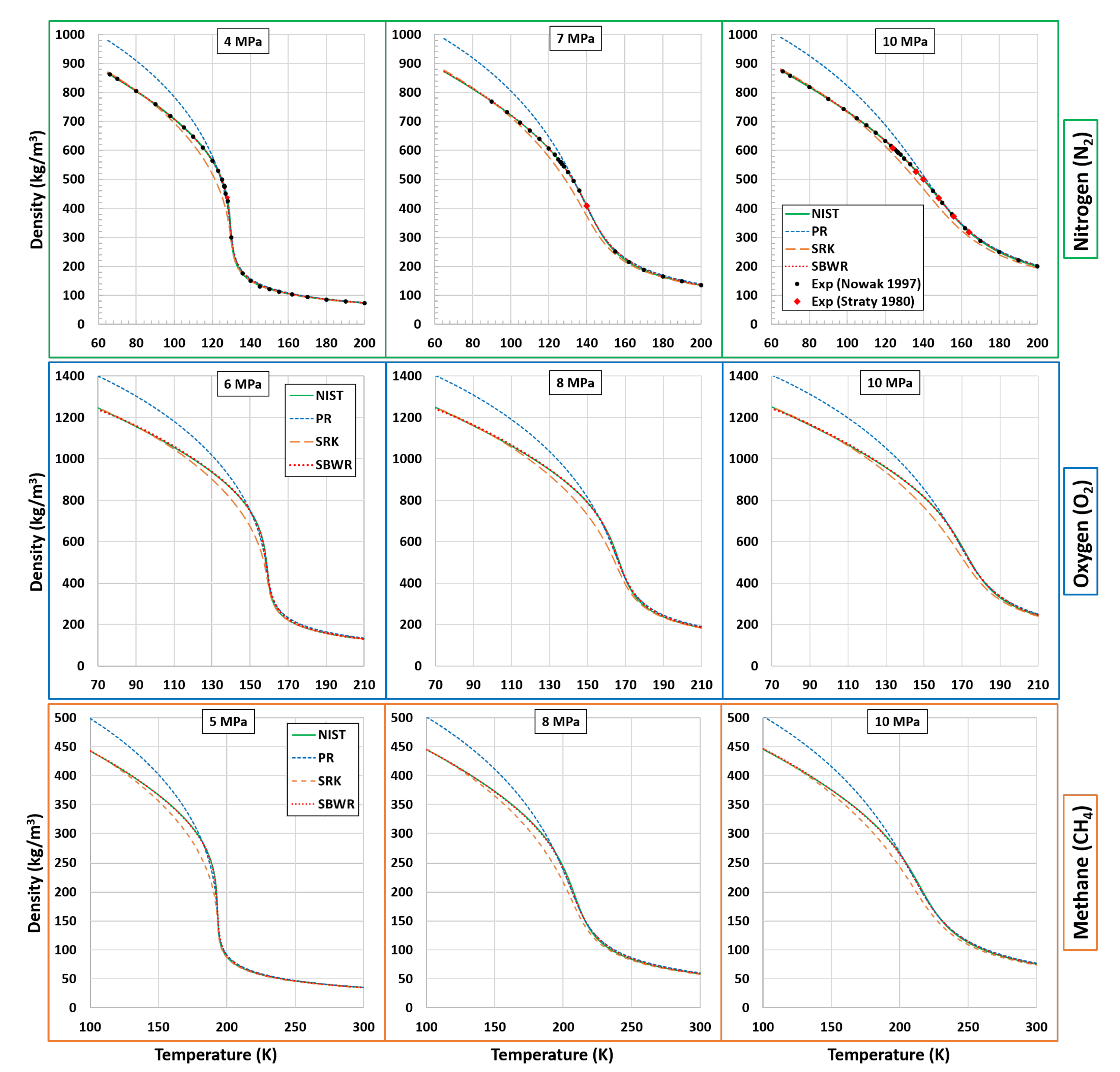
While at subcritical pressures the EoS can return up to 3 roots (consisting of both real and imaginary) in the regions of VLE (vapour-liquid equilibrium) where the minimum root corresponds to liquid phase and the maximum root corresponds to the vapour/gas phase, at supercritical pressures only one positive real root exists for the cubic EoS due to the existence of singular liquid phase below and supercritical phase above the critical temperature. To assess the performance of the real fluid EoS (PR, SRK and SBWR) along with Chung et al.’s method, their estimation of isobaric thermophysical properties for popular cryogenic fluids (N${}_2$, O${}_2$ and CH${}_4$) are presented below at a near-critical supercritical pressure, intermediate supercritical pressure and a high supercritical pressure ($>=$2$P_c$) and compared against the accurate NIST thermophysical property database [18].

Table 2. Table of respective supercritical pressures of three cryogenic fluids (N${}_2$, O${}_2$ and CH${}_4$) for which the thermophysical properties were estimated using EoS and the EoS–Chung model, where $P_c$ is the critical pressure and $P_r$ is the reduced pressure of the respective fluid.

Fluid	Near-Critical		Super-Critical		High		${\mathit{P}}_{\mathit{c}}$
	P (MPa)	${\mathit{P}}_{\mathit{r}}$ ( P/${\mathit{P}}_{\mathit{c}}$)	P (MPa)	${\mathit{P}}_{\mathit{r}}$ (P/${\mathit{P}}_{\mathit{c}}$)	P (MPa)	${\mathit{P}}_{\mathit{r}}$ (P/${\mathit{P}}_{\mathit{c}}$)	(MPa)
N${}_2$	4	1.2	7	2.1	3	2.9	3.396
O${}_2$	6	1.2	8	1.6	10	2	5.043
CH${}_4$	5	1.1	8	1.7	10	2.2	4.599

shows the absolute pressure values examined and their correspondence with the critical values.

5.1. Density

Density estimations at supercritical pressures by PR, SRK and SBWR compared against NIST data for the three cryogenic fluids—nitrogen (N${}_2$), oxygen (O${}_2$) and methane (CH${}_4$) are presented in Figure 2, where the density estimates for N${}_2$ are compared with experimental data by Nowak [65] and Straty [66] as well. Although PR significantly overestimates low temperature liquid densities, it is very accurate in estimating the liquid phase density at temperatures around the pseudoboiling temperature. The entire supercritical phase density is estimated accurately by PR. While SRK is accurate for the most part in estimating the liquid and supercritical phase densities at supercritical pressures, It slightly underestimates their densities around the pseudoboiling temperature. On the other hand, SBWR estimates the liquid and supercritical phase density of all the three cryogenic fluids—N${}_2$, O${}_2$ and CH${}_4$ accurately at all temperatures including around the pseudoboiling temperature at supercritical pressures.

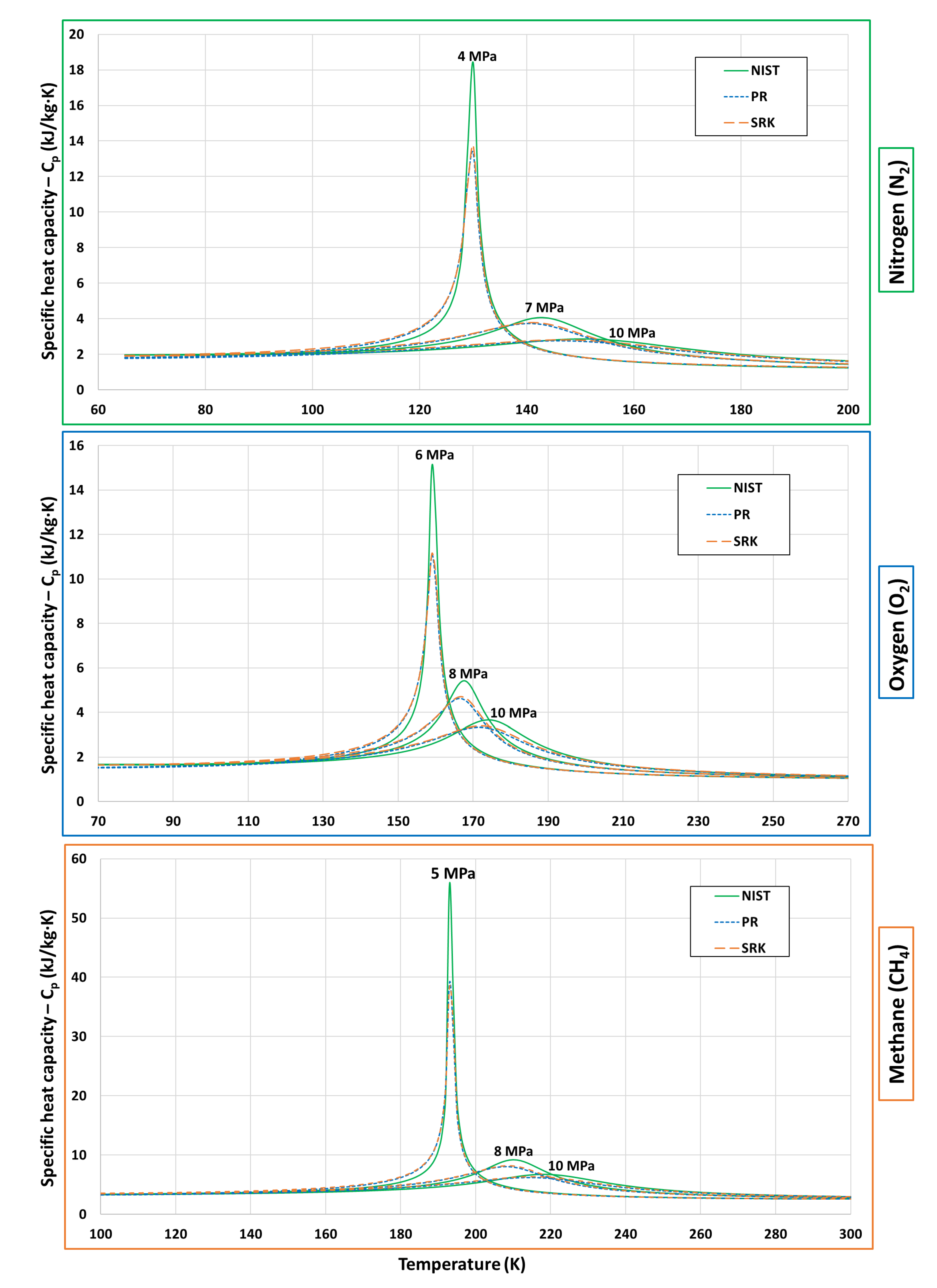
5.2. Thermodynamic Properties-Enthalpy and Specific Heat Capacity

As mentioned earlier, due to the lack of available methods for thermodynamic property derivations from SBWR EoS, only PR and SRK EoS are presented and compared against NIST data. The thermodynamic properties—enthalpy and specific heat capacity of nitrogen (N${}_2$), oxygen (O${}_2$) and methane (CH${}_4$)—estimated by the PR and SRK at supercritical pressures are presented in Figure 3 and Figure 4. The enthalpy estimates by both PR and SRK at supercritical pressures are very accurate when compared against NIST. Though upon taking a closer look at Figure 3, one can find small deviations in PR and SRK around the pseudoboiling temperature where steep changes in enthalpy occur. This is particularly more noticeable for the low supercritical pressures, i.e., just above $P_c$. On the other hand, although the liquid and supercritical phase specific heat capacities of all the three cryogenic fluids are estimated accurately by both PR and SRK for most of the temperature range, there is considerable underestimation around the specific heat capacity peaks located at the pseudoboiling temperature, particularly at low supercritical pressures just above $P_c$.

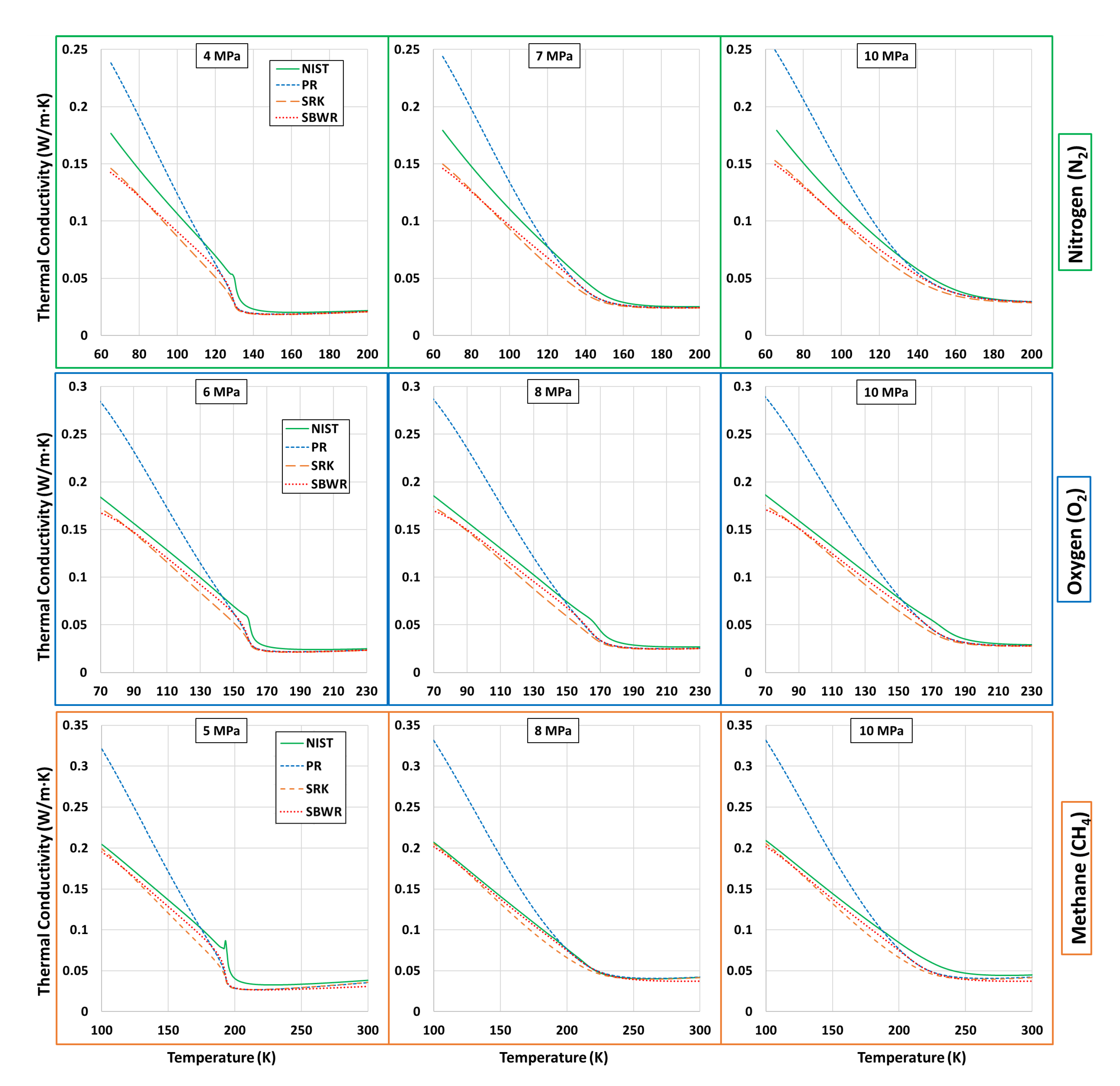
5.3. Transport Properties-Viscosity and Thermal Conductivity

The transport properties—viscosity and thermal conductivity—estimated by Chung et al.’s transport model along with all the EoS-PR, SRK and SBWR for the cryogenic fluids - nitrogen (N${}_2$), oxygen (O${}_2$) and methane (CH${}_4$) at supercritical pressures are presented in Figure 5 and Figure 6 respectively. PR (along with Chung et al.’s model) considerably overestimates low temperature liquid phase viscosity for all the three cryogenic fluids as seen in the Figure 5. Though, the entire supercritical phase viscosity and liquid phase viscosity close to the pseudoboiling point temperature are estimated accurately by PR. SRK (along with Chung et al.’s model) on the other hand manages to estimate the entire liquid and supercritical phase viscosities accurately. SBWR presents with similar excellent accuracy as that of SRK in estimating the viscosities. Similar to its viscosity predictions, PR (along with Chung et al.’s model) considerably overestimates low temperature liquid phase thermal conductivity for all the three cryogenic fluids as seen in the Figure 6. While SRK and SBWR are relatively more accurate in predicting the liquid phase thermal conductivity, at very low temperatures SRK estimates are relatively more accurate whereas around the pseudoboiling temperature SBWR estimates are more accurate. The high temperature supercritical phase thermal conductivity on the other hand is relatively better estimated by all the EoS in a similar manner, though the drastic changes around the pseudoboiling temperature particularly at near critical pressures is not captured by any of the EoS accurately.

5.4. Summary

In general, for the entire range of temperatures and supercritical pressures SRK is more accurate than PR in predicting all the thermophysical properties. However, if lower temperature liquid phase is not of interest, then PR is a better choice than SRK in estimating thermophysical properties of liquid phases and supercritical phase very close to $T_c$, i.e., the pseudoboiling region, whereas the non-cubic SBWR is more accurate than the cubic EoS (PR and SRK explored in this research) in estimating fluid’s density and even the transport properties throughout all supercritical pressures and temperatures. However, since the formulation to estimate thermodynamic properties using SBWR does not exist in the literature, It would be of much interest to cryogenics that thermodynamic property derivations from SBWR is formulated to estimate all the required thermophysical properties. The deviations in transport properties (thermal conductivity in particular) by SBWR-Chung reveals that these are limitations of Chung et al.’s model in itself, as the SBWR density estimates are very accurate.

6. CFD Simulations of Cryogenic Fluids at Supercritical Pressures

In CFD, complex fluid flows are predicted through the solution of the governing equations, i.e., conservation of mass, momentum and energy. With respect to the Finite Volume Method (FVM)—the most popular discretisation method in CFD—the partial differential of these governing equations in the conservative form are solved over discrete control volumes. The partial differential of these conservation equations are given in Equations (7)–(9).

The mass conservation as continuity equation:

$$\frac{\partial \rho }{\partial t}+\nabla ·\left(\rho \mathbf{U}\right)=0,$$

(7)

where $\rho$ is density, t is time and $\mathbf{U}$ is the velocity vector.

The momentum conservation as momentum equation is:

$$\frac{\partial \rho \mathbf{U}}{\partial t}+\nabla ·\left(\rho \mathbf{UU}\right)=-\nabla p+\nabla ·\tau +{\mathbf{f}}_{\mathbf{b}},$$

(8)

where, in addition to the previously defined, $\tau$ denotes the viscous stress tensor and ${\mathbf{f}}_{\mathbf{b}}$ accounts for the body forces.

The energy conservation as energy equation in terms of total energy is:

$$\frac{\partial }{\partial t}\left(\rho E\right)+\nabla ·\left(\rho \mathbf{U}E\right)=-\nabla ·q-\nabla ·\left(p\mathbf{U}\right)+\nabla ·(\tau ·\mathbf{U})+Q+{\mathbf{f}}_{\mathbf{b}}·\mathbf{U},$$

(9)

where, in addition to the previously defined, E is total energy, q is heat flux and Q represents heat sources and sinks

In the above momentum equation, the viscous stress tensor $\tau$ requires as input the viscosity $\mu$. Whereas the total energy E in the energy equation can be constituted in terms of internal energy e and kinetic energy K as $E=e+K$ or in terms of enthalpy h and kinetic energy as $E=h-p/\rho +K$, where the kinetic energy term can be further expanded to $K=u^2/2$. The enthalpy h can also be further expanded in terms of specific heat capacity $C_p$ and temperature T to obtain energy equation in terms of temperature [67]. The thermal conductivity is utilised to determine the heat flux q according to Fourier’s law as $q=-k\nabla T$ where k is the thermal conductivity and T is the temperature. As a result, it can be seen that the various different thermophysical properties have their respective role in these conservation equations.

In many CFD simulations of fluids at atmospheric and subcritical pressures, simplified forms based on constant fluid property assumptions are usually utilised. For CFD studies of cryogenic fluids at supercritical pressures, even at isobaric conditions, the conservation equations are solved in general form without simplifications (apart from the body forces and heat sources/sinks), to account for the continuously varying thermophysical properties [5,21,23,24,59,68,69,70]. These equations are then required to be coupled with real fluid thermophysical models such as real fluid EoS, such that based on the local temperature or state of the fluid, the thermophysical properties are updated at each time step. However to mitigate the stability and deviation issues arising due to the non linearity in thermophysical properties estimated by real fluid EoS, multiple updates (within the same time-step) of thermophysical properties before and after the solution of governing equations are suggested [22,24,59].

In the case of cryogenic fluids at supercritical pressures, the absence of discontinuity between liquid and supercritical fluid phases (seen earlier in Section 2) dictates the treatment of the phases. Even if there are two phases present (liquid and supercritical phase) in reality only one specie is involved. Characteristic of this scenario are the experiments of liquid nitrogen injection into supercritical nitrogen (although referred as GN${}_2$) by Mayer et al. [10]. For these cases, a single set of mass, momentum and energy equation with no additional transport equations is sufficient to simulate the flow and is referred as single-specie approach [23,24,69,71]. However, when more than one cryogenic fluids at supercritical pressures are involved such as liquid oxygen injected coaxially with methane in [21] or liquid oxygen with hydrogen in [72], it is necessary to solve additional equation/s for specie continuity. This method where two different fluids or phases are approximated as a single fluid for mass, momentum and energy continuity with separate treatment for fluid continuity is known as the one-fluid (or single-fluid) approach [5,19,20,21,70]. The main advantage of one-fluid approach for cryogenic fluids at supercritical pressures is that it can be used for multi-specie cases as well as single-specie cases. In the one-fluid approach although single set of mass, momentum and energy equations are solved for the mixture, additional continuity equations in terms of mass fraction [21,70] or mixture fraction [19,20] or even volume fraction [5] with inter-diffusion are solved for fluid continuity. Here, the injected and the ambient/chamber fluid are considered separately whether they are of the same or different species, and the properties of the mixture constituting both injected and chamber fluid are calculated through various mixing or averaging rules/methods such as Van der Waals mixing rules [21], mole fraction weighted average [70], volume fraction weighted average [5], etc. Regardless of the variations across single-fluid approaches they have all shown to perform well against experimental data such as the case in [10] of single-specie cryogenic fluid injection of liquid nitrogen into supercritical nitrogen at supercritical pressures, when coupled with an appropriate real fluid thermophysical model [5,19,20,21,70]. It should be pointed out that the one(single)-fluid’s approach’s accuracy in simulation of multi-specie cryogenic fluid cases is largely unknown due to the unavailability of detailed quantitative experimental data to compare.

7. Real Fluid EoS in CFD Simulations of Cryogenic Fluids at Supercritical Pressures

Among the recent CFD studies of cryogenic fluids at supercritical pressures [19,20,21,22,24,46,59,69,70,73], cubic EoS—especially PR and SRK—remain the most popular choice for numerical simulations. Their relative simplicity and their applicability to various fluids in addition to their ability to predict mixture properties is a significant advantage. While the cubic EoS are simple and perform well at all regions including the vapour-liquid equilibrium and transcritical regions, they still have their respective shortcoming. Although SRK and PR both predict the density of the gas and high temperature supercritical phases accurately, the PR deviates largely around low temperature liquid phase, whereas the SRK’s accuracy decreases around the critical and pseudoboiling points, as usually previewed by researchers simulating cryogenic fluids [19,20,21,23] and also as shown by our analysis above. While the volume translation methods [74,75] have been shown to increase the accuracy of PR estimations significantly, the associated complexity in obtaining analytical solutions of departure functions for thermodynamic properties has limited its applicability in CFD [22]. Both PR and SRK have also been found to significantly underestimate the specific heat capacity peaks at supercritical pressures [76]. Other non cubic, empirical EoS such as Younglove’s [28,29] Modified Benedict Webb Rubin (MBWR) EoS have also been used but on a more limited basis (see for example [77]) due to the associated complexity. Unlike the cubic EoS, the MBWR EoS as mentioned earlier requires a large number of empirical parameters specific to each fluid, which significantly limits its applicability to CFD codes since they need to be imported a priori.

Table 3 summarises various EoS and thermophysical models used by researchers for CFD simulations of cryogenic injection at supercritical pressures which are compared against cryogenic injection experiments. Referring to the table, the notation the thermophysical properties column as “PR or SRK derived” represents that the thermodynamic properties were obtained from the departure functions and the respective EoS, whereas the transport properties are obtained through the mentioned supplemented models. As already mentioned while the cubic EoS on their own cannot estimate the transport properties, some EoS such as the MBWR have independent equations and empirical parameters to estimate transport properties. Regardless, the Chung et al.’s [36] method along with cubic EoS is the most popular choice as seen in the table.

The density measurements from experiments of single-specie cases of liquid nitrogen injected into supercritical nitrogen at supercritical pressures by Mayer [10] is a popular choice for validation of the CFD studies, where the injected liquid transitions into a supercritical fluid and then diffuses into the supercritical environment. With respect to the performance of PR and SRK in these CFD studies, although some researchers prefer SRK over PR for their simulations [24,69] and vice-versa [46,70,73], many of the earlier researchers have performed simulations utilising both PR and SRK to compare their respective effects on the simulations of cryogenic jets in supercritical environment [19,20,21,59]. Both PR and SRK when used in CFD studies were able to predict the density variations associated with pseudo-boiling behaviour of the injected liquid as it transitions and the flow develops into a jet. It was observed that the difference between PR and SRK in simulation of such cryogenic jets were insignificant and both of them were in good agreement with experiments. Some differences are observed in centreline density predictions of liquid nitrogen by PR and SRK EoS, [19,20,21]. Kim et al. [19] has further highlighted the differences of PR and SRK on turbulent transport properties in CFD where PR predicts a higher turbulent viscosity for the jet at the pseudoboiling regions, whereas SRK results in a higher turbulent kinetic energy. However, there is almost no difference between CFD results utilising PR and SRK in estimating the spreading rate [20] or the density decay of the jet further down [19,20,21]. The comparison of PR and SRK EoS in these CFD studies against experiments led some researchers to state the superiority of one EoS over the other. These conclusions should be taken with caution because of the large uncertainties in the experimental measurements themselves. Very few simulations utilise ideal gas EoS alongside PR and/or SRK for simulations. They were used to mostly demonstrate that the real fluid behaviour associated with the transition of fluid properties around the pseudo-boiling regions cannot be predicted by the ideal EoS [19,20,24].

Table 3. Table summarising the EoS and thermo-physical models used in some past numerical simulation of cryogenic fluids. The last column refers to the experiments against which the predicted behaviour of the cryogenic jets is compared.

Simulation	EoS	Thermodynamic	Transport	Experiment
		Properties	Model	Simulated
Mayer et al. [10] (2003)	Lee-Kesler		Chung et al. [36]	Mayer et al. [10]
Zong et al. [68] (2004)	SRK	SRK derived	32 term BWR [37,38]	Chehroudi et al. [78]
Schmitt et al. [71] (2010)	PR	PR derived	Chung et al. [36]	Mayer et al. [10]
Kim et al. [19] (2011)	PR and SRK	PR and SRK	Chung et al. [36]	Telaar et al. [11]
		derived		Oschwald et al. [15]
Park [20] (2012)	PR and SRK	PR and SRK	Chung et al. [36]	Telaar et al. [11]
		derived		Oschwald et al [15]
Petite et al. [21] (2013)	PR and SRK	PR and SRK	Chung et al. [36]	Mayer et al. [10]
		derived
Pfitzner et al. [73] (2013)	PR	PR derived	Chung et al. [36]	Telaar et al. [11]
				Mayer et al. [10]
Hickey [46] (2014)	PR	PR derived	Chung et al. [36]	Braman et al. [12]
Muller et al. [22] (2016)	PR	PR derived	Chung et al. [36]	Mayer et al. [10]
Banuti et al. [77] (2016)	MBWR based	MBWR based	MBWR based	Mayer et al. [10]
	data tabulation	data tabulation	data tabulation [28,29]	Branam et al. [79]
Li et al. [24] (2018)	SRK	SRK derived	Viscosity-	Telaar et al. [11]
			Zéberg-Mikkelsen et al. [40]	Mayer et al. [10]
			Thermal conductivity
			-Vasserman et al. [39]
Lagarza-Cortés et al. [69] (2019)	SRK	SRK derived	Chung et al. [36]	Mayer et al. [10]
Ningegowda et al. [70] (2020)	PR	PR derived	Chung et al. [36]	Mayer et al. [10]
Ma et al. [59] (2021)	PR and SRK	PR and SRK	Viscosity-
		derived	Zéberg-Mikkelsen et al. [40]	Mayer et al. [10]
			Thermal conductivity
			-Vasserman et al. [39]

Table 3. Table summarising the EoS and thermo-physical models used in some past numerical simulation of cryogenic fluids. The last column refers to the experiments against which the predicted behaviour of the cryogenic jets is compared.

Simulation	EoS	Thermodynamic	Transport	Experiment
		Properties	Model	Simulated
Mayer et al. [10] (2003)	Lee-Kesler		Chung et al. [36]	Mayer et al. [10]
Zong et al. [68] (2004)	SRK	SRK derived	32 term BWR [37,38]	Chehroudi et al. [78]
Schmitt et al. [71] (2010)	PR	PR derived	Chung et al. [36]	Mayer et al. [10]
Kim et al. [19] (2011)	PR and SRK	PR and SRK	Chung et al. [36]	Telaar et al. [11]
		derived		Oschwald et al. [15]
Park [20] (2012)	PR and SRK	PR and SRK	Chung et al. [36]	Telaar et al. [11]
		derived		Oschwald et al [15]
Petite et al. [21] (2013)	PR and SRK	PR and SRK	Chung et al. [36]	Mayer et al. [10]
		derived
Pfitzner et al. [73] (2013)	PR	PR derived	Chung et al. [36]	Telaar et al. [11]
				Mayer et al. [10]
Hickey [46] (2014)	PR	PR derived	Chung et al. [36]	Braman et al. [12]
Muller et al. [22] (2016)	PR	PR derived	Chung et al. [36]	Mayer et al. [10]
Banuti et al. [77] (2016)	MBWR based	MBWR based	MBWR based	Mayer et al. [10]
	data tabulation	data tabulation	data tabulation [28,29]	Branam et al. [79]
Li et al. [24] (2018)	SRK	SRK derived	Viscosity-	Telaar et al. [11]
			Zéberg-Mikkelsen et al. [40]	Mayer et al. [10]
			Thermal conductivity
			-Vasserman et al. [39]
Lagarza-Cortés et al. [69] (2019)	SRK	SRK derived	Chung et al. [36]	Mayer et al. [10]
Ningegowda et al. [70] (2020)	PR	PR derived	Chung et al. [36]	Mayer et al. [10]
Ma et al. [59] (2021)	PR and SRK	PR and SRK	Viscosity-
		derived	Zéberg-Mikkelsen et al. [40]	Mayer et al. [10]
			Thermal conductivity
			-Vasserman et al. [39]

8. Alternative Approaches of Modelling Thermophysical Properties

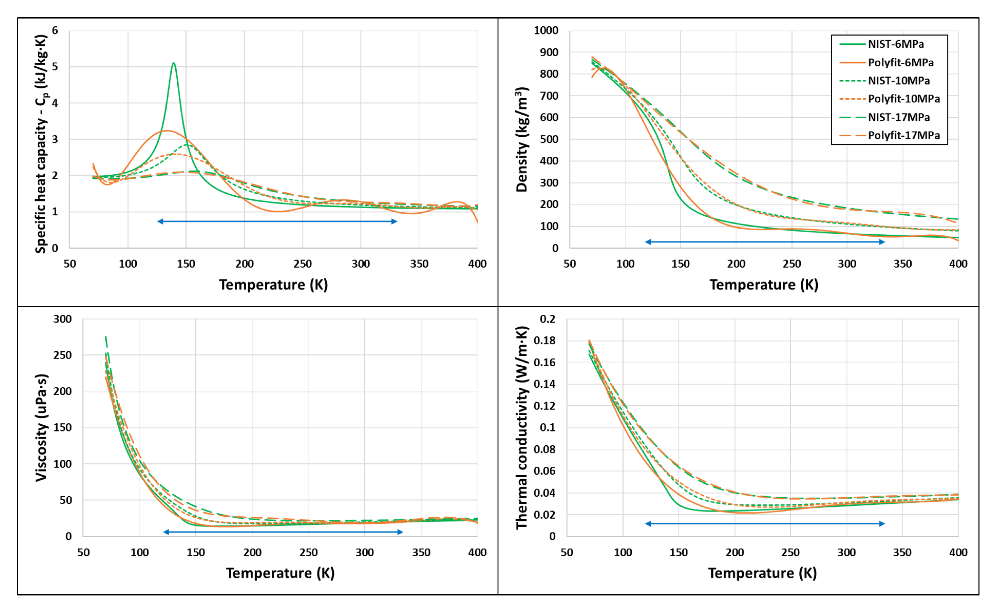
8.1. Polynomial Fitting of Data

While other EoS models require extensive coding to implement in numerical simulations, the ease of access to NIST data [18] as well as CoolProp [30] containing accurate thermophysical properties of various cryogenic fluids enables methods based on polynomial fitting to be used with sufficient accuracy. The isobaric, isochoric or isothermal thermophysical properties from NIST can be regressed into polynomial form of any degree. The accuracy of the polynomial fit to the data increases with the increase in the degree of the polynomial. Care should be taken to include sufficient significant figures in the coefficients of the polynomial to return accurate estimates. These polynomials can then be used as “equations” for thermophysical properties in numerical simulations. For example one of the most popular current softwares for CFD, OpenFOAM [80] has a built-in thermophysical model which allows the use of up to 8th order polynomials. It should be noted that high order polynomials might deviate from the fitted data outside of the fit domain, however this can be counterbalanced by fitting the polynomials over a larger range than that used for simulation. Figure 7 shows the polynomial fitting of NIST data of N${}_2$ from [4], used in supercritical cryogenic simulations [5]. These supercritical cryogenic simulations also include Mayer et al. [10] `case 9’ where cryogenic N${}_2$ was injected into an isobaric chamber maintained at 6 MPa supercritical pressure. The injection temperature is more than 120 K and the chamber temperature is 298 K. By using NIST data for an extended range of 70 K–400 K sufficient accuracy was ensured. Although the specific heat capacity at constant pressure deviates by around 40% at the pseudo-boiling point for 6 MPa, for higher supercritical pressures the peak is lower and a better polynomial fit is observed. Excluding the specific heat capacity, other thermophysical properties utilising the polynomial fitting model show sufficient accuracy even at near critical pressures where a steep change in these thermophysical properties is present (see Figure 7).

8.2. Tabulation

Tabulated properties are another alternative to EoS in numerical simulations to accurately model the thermophysical properties of the fluid under consideration. The NIST thermophysical property database [18] and data from CoolProp [30] can be used as dataset for the base of tabulation of common cryogenic fluids at wide range of pressure and temperature conditions. It should be pointed though that the tabulation method is not limited to these databases alone. Any EoS estimates can be tabulated to reduce the computational time. For example, a two-dimensional tabulation model of Temperature and (required) Thermophysical properties obtained from a multi-EoS real fluid model has been demonstrated recently by Jafari et al. [81] to simulate isobaric cryogenic and supercritical conditions with increased computational efficiency while avoiding a loss in effective accuracy, when compared to the respective EoS. These simulations by Jafari et al. demonstrated the capability to capture the condensation of H${}_2$ in the case of binary fluid case of LO${}_X$ injected with coaxial H${}_2$ at supercritical pressures of LO${}_X$. The local reduction in the critical point as the LO${}_X$ forms a mixture with H${}_2$, denoting local subcritical mixing regimes within an overall supercritical environment condition was also reflected in the simulation results, providing evidence for detailed capture of thermodynamic phenomena while using tabulation models. In contrast, Yang et al. [82] utilised a pre-built 2D tabulation model corresponding to the case, based solely on thermophysical property data from experiments in simulation of LO${}_X$ and CH${}_4$ mixing at supercritical conditions. Yang et al. demonstrated that such tabulation models can accelerate the computational simulation by a factor of 2, and evaluation of the properties by a factor of 10, while demonstrating excellent accuracy against the chosen benchmark case.

Though the recent simulations by other researchers have been limited to 2D tabulation models of (Temperature-Thermophysical property) for isobaric cases, it is viable to even utilise a 3D tabulation model of (Pressure–Temperature–Thermophysical property) for non-isobaric (and non-isothermal) cases such as when applied to the simulation of compression chambers in RSCE mentioned in the introduction. Such 3D tabulation models should also result in considerable computational acceleration (with respect to EoS), although with increase in dimensions of the tabulation model the advantage in computational acceleration will decrease. Another advantage of the tabulation model is that it can be utilised for any fluid, through tabulation of thermophysical property from other complex EoS or databases, while avoiding the extensive coupling necessary for the EoS to be implemented effectively in simulations. Correspondingly for simulations consisting of different type of fluids, it also provides leverage to select specific EoS for each fluid in simulation depending on the accuracy requirements. Nevertheless, additional research is necessary to understand the impact of interpolation method and discretisation of the tabulated data on simulations.

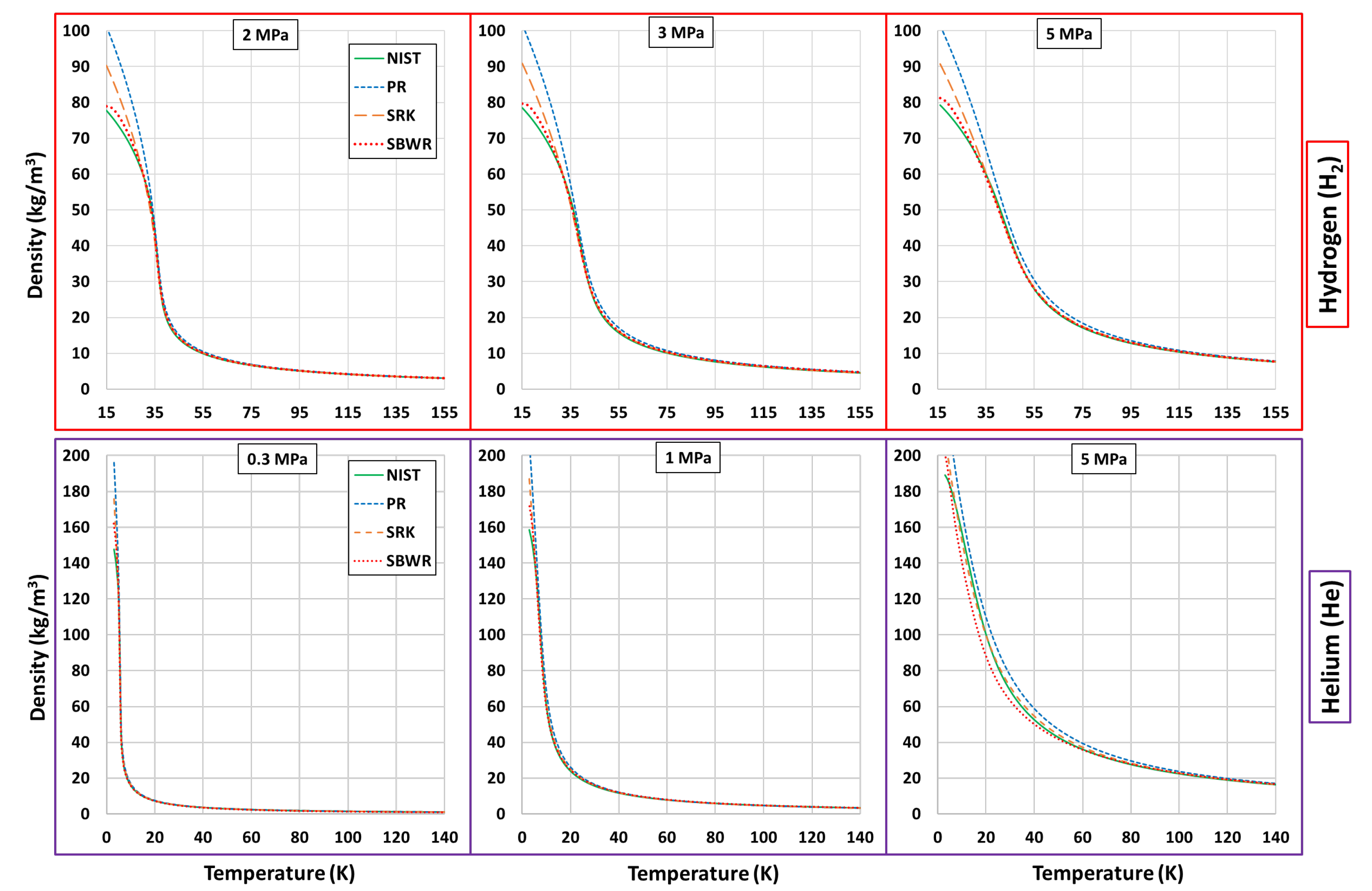
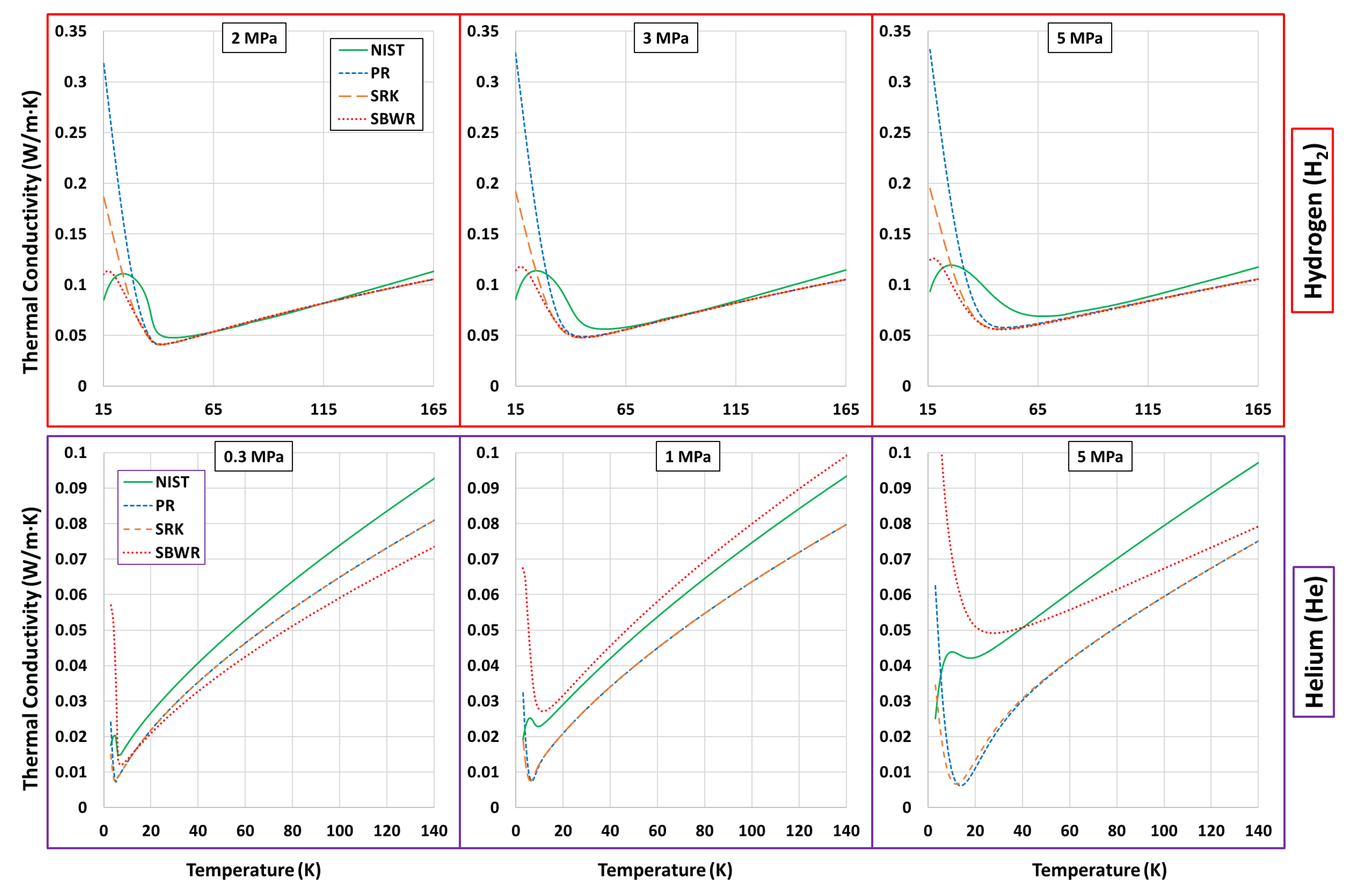
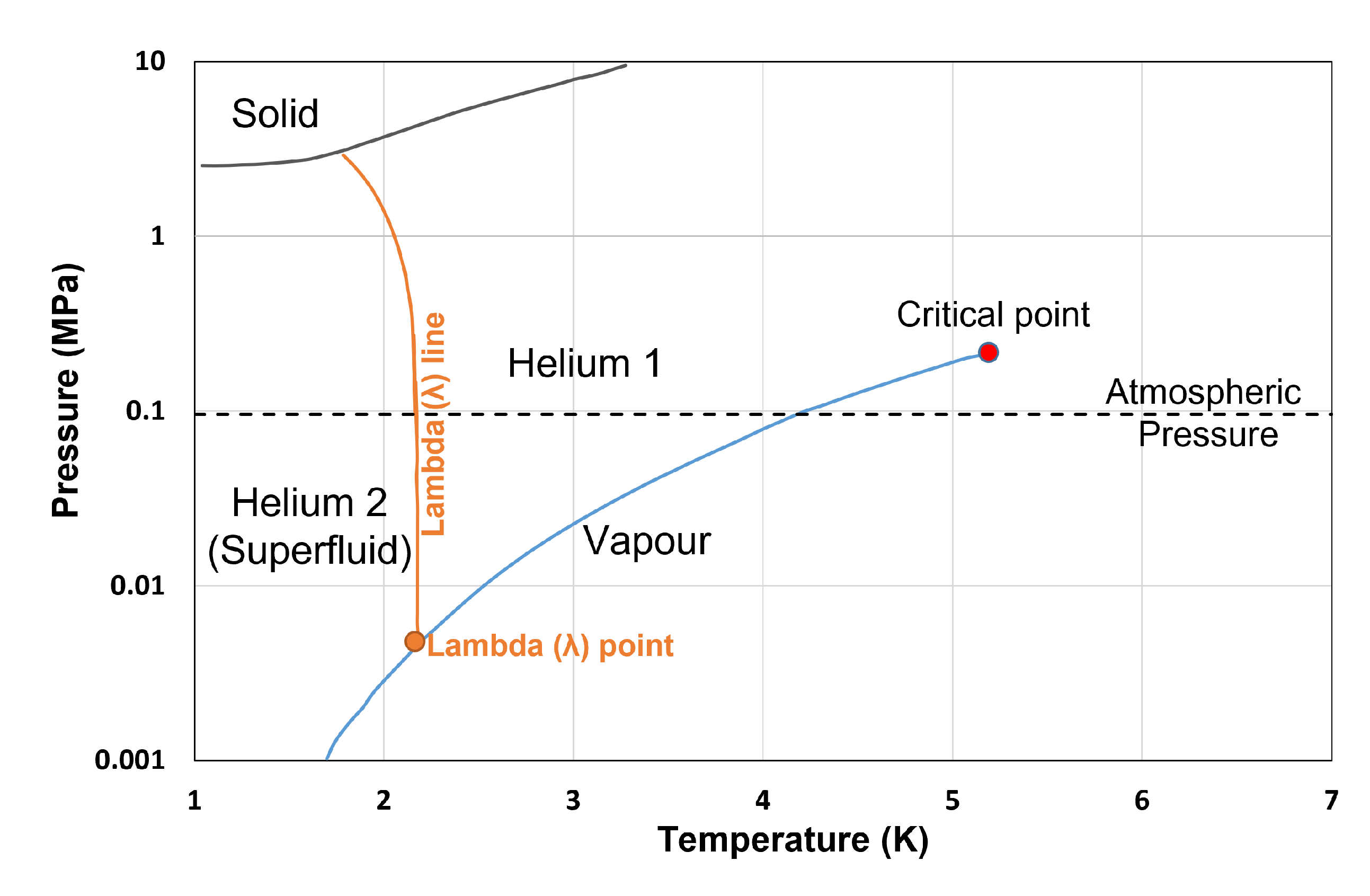
9. Discussion on Cryogenic Fluids with Quantum Effects

While the above presented thermophysical properties trends are common across most cryogenic fluids and their transition at supercritical pressures, due to quantum effects at low temperatures, there are exceptions that will be discussed briefly here. Specifically, helium-4, the prevalent isotope of helium and hydrogen show significant deviations from the general trends. Helium (i.e., helium-4) is unique as it exists as a superfluid (zero viscosity) liquid phase at a very narrow range of very low temperatures. The phase diagram of helium (Figure 8) shows the superfluid liquid phase (helium 2) and the general liquid phase (helium 1) existence regions, along with the lambda($\lambda$)-curve (also known as the lambda-line). Instead of the triple point, the lambda ($\lambda$) point is considered the lower limit of thermodynamic functions and EoS for helium (He) [83], as quantum effects tend to be significant at very low temperatures (below the $\lambda$-point temperature) [1] where it also exhibits superfluidity.

In the case of hydrogen (H${}_2$), the quantum effects are observed through its spin isomers and the much higher characteristic rotational temperature. Any amount of H${}_2$ consists of both of its molecular isomers: ortho- and para-hydrogen, whose composition depends on the equilibrium temperature. Ortho- and para-spin isomers having different nuclear spin configuration, have different ground state energy levels [85]. As a result, the thermodynamic properties of ortho- and para-hydrogen deviate significantly (up to 30%) at temperatures up to 300 K [83]. While at low temperatures (below 77 K) the composition is dominated by para-hydrogen, at higher temperatures (above 77 K) the composition is dominated by ortho-spin isomer of hydrogen. The transition from ortho- to para-hydrogen and vice-versa is not spontaneous. Increase/decrease in temperature slowly drives the ortho- to para- (and vice-versa) transition over time (which can even take many days) to achieve a new equilibrium composition. This variance in composition of para:ortho from 100:0 at 0 K, to 25:75 at higher temperatures requires the properties to be calculated according to the equilibrium composition of ortho- and para-hydrogen with respect to temperature. (At 77 K the ortho to para composition is exactly 50:50). Normal hydrogen, considered as a pure fluid for practical purposes, is a mixture of ortho- and para-hydrogen in 25:75 composition [86]. Another interesting feature underlining the influence of quantum effects in H${}_2$ is the rotational contribution to internal energy of diatomic molecules. Unlike other single-component diatomic molecules such as N${}_2$ and O${}_2$ whose rotational temperature is much lower at 2–3 K, the characteristic rotational temperature of H${}_2$ is 87.6 K, above which the rotational excitation starts to contribute to the internal energy of diatomic molecules [55]. The maximum rotational energy for diatomic H${}_2$ though, is only attained at even higher temperatures (around 200 K) after the complete actuation of rotation. As a result, the internal energy of H${}_2$ lies between that of monoatomic and diatomic at temperatures within this range. Thus, the thermodynamic properties of hydrogen are also observed to deviate significantly at lower temperatures from the ones expected for diatomic fluids.

Thermophysical Property Estimation of Hydrogen (H${}_2$) and Helium (He) Using Common Real Fluid EoS

The density estimations of hydrogen (H${}_2$) and helium (He) through PR, SRK and SBWR provide sufficient accuracy for most of the supercritical range. However, the liquid phase and lower temperature supercritical phase estimations are affected by the quantum effects and show significant deviations (see Appendix B). These inaccuracies in density are expected to also affect the thermodynamic properties since the thermodynamic properties are in reality obtained from EoS. The transport properties estimations of H${}_2$ and He by these EoS also show large deviations and are not able to capture the trends in the curve at the liquid phase. As a result, those few CFD simulations involving hydrogen (H${}_2$) at supercritical pressures which although employ PR or SRK EoS for the high temperature (well above critical temperature) supercritical phase [87,88], the deviations due to quantum influence at liquid phase are unlikely to be significant.

10. Conclusions

The continuous variation in thermophysical properties associated with the phase transition of cryogenic fluids at supercritical pressures and the thermal as well as inertial influence in the evolution of such fluids in a supercritical environment requires appropriate real fluid thermophysical property models for density as well as thermodynamic and transport properties, to be able to simulate the evolution of such fluids adequately.

While the cubic EoS—particularly PR and SRK—are able to estimate density and thermodynamic properties—enthalpy and specific heat capacity—additional models are required for the estimation of transport properties—thermal conductivity and viscosity. When used along with Chung et al.’s model for transport properties, although SRK is more accurate than PR in predicting these thermophysical properties for a wider range of liquid to supercritical phases at supercritical pressures, PR is more accurate around the pseudoboiling region. The non cubic EoS SBWR, on the other hand, although being more accurate than PR and SRK for the entire range of temperatures and phases at supercritical pressures, is limited by the complexity in obtaining thermodynamic properties.

From the review of past single-specie and one-fluid CFD approaches to simulating cryogenic fluids at supercritical pressure conditions, both PR and SRK along with Chung et al.’s transport properties model are commonly utilised due to the requirement of minimal fluid specific parameters (only critical properties are needed) and are deemed to be sufficiently accurate for predicting the evolution of cryogenic fluids in CFD studies. Although there are other, more complex non cubic EoS available in the literature, due to the high cost of implementation associated with the requirement of several fluid specific parameters, they are scarcely utilised in CFD simulation of cryogenic fluids. On the other hand, data-based alternate thermophysical models such as polynomial fitting and tabulation are easier to implement and also reduce the computational cost and perform on a par with, or even better than, EoS when utilised within their limitations. It is also worth noting that the uncertainty in the few available experiments to compare the simulation with makes it hard to ascertain which of these real fluid EoS are more accurate for CFD simulations, especially considering that other sources of error (grid accuracy, discretisation etc) affect the final predictions. Regardless, it is clear that an appropriate real fluid model needs to be utilised for meaningful simulations of cryogenic fluids at supercritical pressures that can accurately reproduce the fluid properties that are characterised by steep gradients, sharp peaks, and which are non-monotonous. While the cubic EoS models can be reliably utilised for several common cryogenic fluids, these models are rendered inadequate to estimate the liquid phase thermophysical properties of cryogenic fluids in which quantum effects are important, such as hydrogen and helium.

References

1. Radebaugh, R.; Bar-Cohen, Y. Low Temperature Materials and Mechanisms: Applications and Challenges. In Low Temperature Materials and Mechanisms, 1st ed.; Bar-Cohen, Y., Ed.; CRC Press: Boca Raton, FL, USA, 2016; Chapter 14. [Google Scholar] [CrossRef]
2. Owen, N.; Treccarichi, F.; Atkins, A.; Selvaraj, A.; Barnes, D.; Besant, T.; Morgan, R. A Practical Recuperated Split Cycle Engine for Low Emissions and High Efficiency. In Proceedings of the 14th International Conference on Engines & Vehicles, Naples, Italy, 15–19 September 2019. [Google Scholar] [CrossRef]
3. Jaya Vignesh, M.; Harvey, S.; Atkins, A.; Atkins, P.; De Sercey, G.; Heikal, M.; Morgan, R.; Vogiatzaki, K. Use of cryogenic fluids for zero toxic emission hybrid engines. In Internal Combustion Engines and Powertrain Systems for Future Transport 2019, 1st ed.; CRC Press: London, UK, 2020; pp. 117–130. Available online: https://www.taylorfrancis.com/books/oa-edit/10.1201/9781003023982/internal-combustion-engines-powertrain-systems-future-transport-2019-imeche (accessed on 15 October 2022). [CrossRef]
4. Jaya Vignesh, M.; Tretola, G.; Morgan, R.; Sercey, G.d.; Atkins, A.; Vogiatzaki, K. Understanding Sub and Supercritical Cryogenic Fluid Dynamics in Conditions Relevant to Novel Ultra Low Emission Engines. Energies 2020, 13, 3038. [Google Scholar] [CrossRef]
5. Madana Gopal, J.V.; Tretola, G.; Morgan, R.; Sercey, G.d.; Lamanna, G.; Vogiatzaki, K. Unpicking the interplay of turbulence, diffusion, and thermophysics in cryogenic jets at supercritical pressures. Phys. Fluids 2021, 33, 077106. [Google Scholar] [CrossRef]
6. Starship. Available online: https://www.spacex.com/vehicles/starship (accessed on 15 October 2022).
7. Mayer, W.O.H.; Schik, A.H.A.; Vielle, B.; Chauveau, C.; Gokalp, I.; Talley, D.G.; Woodward, R.D. Atomization and Breakup of Cryogenic Propellants Under High-Pressure Subcritical and Supercritical Conditions. J. Propuls. Power 1998, 14, 835–842. [Google Scholar] [CrossRef]
8. Chehroudi, B.; Talley, D.; Coy, E. Visual characteristics and initial growth rates of round cryogenic jets at subcritical and supercritical pressures. Phys. Fluids 2002, 14, 850–861. [Google Scholar] [CrossRef]
9. Mayer, W.; Schik, A.; Schweitzer, C.; Schaeffler, M. Injection and mixing processes in high pressure LOX/GH2 rocket combustors. In Proceedings of the 32nd Joint Propulsion Conference and Exhibit, Lake Buena Vista, FL, USA, 1–3 July 1996. [Google Scholar] [CrossRef]
10. Mayer, W.; Telaar, J.; Branam, R.; Schneider, G.; Hussong, J. Raman Measurements of Cryogenic Injection at Supercritical Pressure. Heat Mass Transf. 2003, 39, 709–719. [Google Scholar] [CrossRef]
11. Telaar, J.; Schneider, G.; Hussong, J.; Mayer, W. Cryogenic Jet Injection: Description of Test Case RCM 1. In Proceedings of the 2nd International Workshop on Rocket Combustion Modeling: Atomization, Combustion and Heat Transfer, Lampoldshausen, Germany, 25–27 March 2001. [Google Scholar]
12. Branam, R.; Mayer, W. Length scales in cryogenic injection at supercritical pressure. Exp. Fluids 2002, 33, 422–428. [Google Scholar] [CrossRef]
13. Oschwald, M.; Schik, A. Supercritical nitrogen free jet investigated by spontaneous Raman scattering. Exp. Fluids 1999, 27, 497–506. [Google Scholar] [CrossRef]
14. Oschwald, M.; Schik, A.; Klar, M.; Mayer, W. Investigation of coaxial LN2/GH2-injection at supercritical pressure by spontaneous Raman scattering. In Proceedings of the 35th Joint Propulsion Conference and Exhibit, Los Angeles, CA, USA, 20–24 June 1999. [Google Scholar] [CrossRef]
15. Oschwald, M.; Smith, J.J.; Branam, R.; Hussong, J.; Schik, A.; Chehroudi, B.; Talley, D. Injection of fluids into supercritical environments. Combust. Sci. Technol. 2006, 178, 49–100. [Google Scholar] [CrossRef]
16. Chehroudi, B.; Talley, D.; Coy, E. Initial growth rate and visual characteristics of a round jet into a sub- to supercritical environment of relevance to rocket, gas turbine, and diesel engines. In Proceedings of the 37th Aerospace Sciences Meeting and Exhibit, Hampton, VA, USA, 11–14 January 1999. [Google Scholar] [CrossRef] [Green Version]
17. Chehroudi, B. Recent Experimental Efforts on High-Pressure Supercritical Injection for Liquid Rockets and Their Implications. Int. J. Aerosp. Eng. 2012, 2012, 121802. [Google Scholar] [CrossRef] [Green Version]
18. Lemmon, E.W.; Bell, I.H.; Huber, M.L.; McLinden, M.O. Thermophysical Properties of Fluid Systems. In NIST Chemistry WebBook, NIST Standard Reference Database Number 69; Linstrom, P.J., Mallard, W.G., Eds.; National Institute of Standards and Technology: Gaithersburg, MD, USA, 2022. Available online: https://webbook.nist.gov/chemistry/fluid (accessed on 15 October 2022). [CrossRef]
19. Kim, T.; Kim, Y.; Kim, S.K. Numerical study of cryogenic liquid nitrogen jets at supercritical pressures. J. Supercrit. Fluids 2011, 56, 152–163. [Google Scholar] [CrossRef]
20. Park, T.S. LES and RANS simulations of cryogenic liquid nitrogen jets. J. Supercrit. Fluids 2012, 72, 232–247. [Google Scholar] [CrossRef]
21. Petit, X.; Ribert, G.; Lartigue, G.; Domingo, P. Large-eddy simulation of supercritical fluid injection. J. Supercrit. Fluids 2013, 84, 61–73. [Google Scholar] [CrossRef]
22. Müller, H.; Niedermeier, C.A.; Matheis, J.; Pfitzner, M.; Hickel, S. Large-eddy simulation of nitrogen injection at trans- and supercritical conditions. Phys. Fluids 2016, 28, 015102. [Google Scholar] [CrossRef]
23. Wei, W.; Xie, M.; Jia, M. Large eddy simulation of fluid injection under transcritical and supercritical conditions. Numer. Heat Transf. Part A Appl. 2016, 70, 870–886. [Google Scholar] [CrossRef]
24. Li, L.; Xie, M.; Wei, W.; Jia, M.; Liu, H. Numerical investigation on cryogenic liquid jet under transcritical and supercritical conditions. Cryogenics 2018, 89, 16–28. [Google Scholar] [CrossRef]
25. Magalhães, L.; Carvalho, F.; Silva, A.; Barata, J. Turbulence Modeling Insights into Supercritical Nitrogen Mixing Layers. Energies 2020, 13, 1586. [Google Scholar] [CrossRef] [Green Version]
26. Banuti, D. Thermodynamic Analysis and Numerical Modeling of Supercritical Injection. Ph.D. Thesis, University of Stuttgart, Stuttgart, Germany, 2015. [Google Scholar] [CrossRef]
27. Lemmon, E.W.; Bell, I.; Huber, M.L.; McLinden, M.O. NIST Standard Reference Database 23: Reference Fluid Thermodynamic and Transport Properties-REFPROP, Version 10.0; National Institute of Standards and Technology: Gaithersburg, MD, USA, 2018. [Google Scholar] [CrossRef]
28. Younglove, B.A. Erratum: Thermophysical Properties of Fluids. I. Argon, Ethylene, Parahydrogen, Nitrogen, Nitrogen Trifluoride, and Oxygen. J. Phys. Chem. Ref. Data 1985, 14, 619. [Google Scholar] [CrossRef] [Green Version]
29. Younglove, B.A.; Ely, J.F. Thermophysical Properties of Fluids. II. Methane, Ethane, Propane, Isobutane, and Normal Butane. J. Phys. Chem. Ref. Data 1987, 16, 577–798. [Google Scholar] [CrossRef]
30. Bell, I.H.; Wronski, J.; Quoilin, S.; Lemort, V. Pure and Pseudo-pure Fluid Thermophysical Property Evaluation and the Open-Source Thermophysical Property Library CoolProp. Ind. Eng. Chem. Res. 2014, 53, 2498–2508. [Google Scholar] [CrossRef] [PubMed] [Green Version]
31. Gross, J.; Sadowski, G. Perturbed-Chain SAFT: An Equation of State Based on a Perturbation Theory for Chain Molecules. Ind. Eng. Chem. Res. 2001, 40, 1244–1260. [Google Scholar] [CrossRef]
32. Kunz, O.; Group, E.G.R. The GERG-2004 Wide Range Equation of State for Natural Gases and Other Mixtures: GERG TM15 2007. In Fortschrittberichte VDI/6: Energietechnik; VDI-Verlag: Düsseldorf, Germany, 2007. [Google Scholar]
33. Kunz, O.; Wagner, W. The GERG-2008 Wide-Range Equation of State for Natural Gases and Other Mixtures: An Expansion of GERG-2004. J. Chem. Eng. Data 2012, 57, 3032–3091. [Google Scholar] [CrossRef]
34. Peng, D.Y.; Robinson, D.B. A New Two-Constant Equation of State. Ind. Eng. Chem. Fundam. 1976, 15, 59–64. [Google Scholar] [CrossRef]
35. Soave, G. Equilibrium constants from a modified Redlich-Kwong equation of state. Chem. Eng. Sci. 1972, 27, 1197–1203. [Google Scholar] [CrossRef]
36. Chung, T.H.; Ajlan, M.; Lee, L.L.; Starling, K.E. Generalized multiparameter correlation for nonpolar and polar fluid transport properties. Ind. Eng. Chem. Res. 1988, 27, 671–679. [Google Scholar] [CrossRef]
37. Ely, J.F.; Hanley, H.J.M. Prediction of transport properties. 1. Viscosity of fluids and mixtures. Ind. Eng. Chem. Fundam. 1981, 20, 323–332. [Google Scholar] [CrossRef]
38. Ely, J.F.; Hanley, H.J.M. Prediction of transport properties. 2. Thermal conductivity of pure fluids and mixtures. Ind. Eng. Chem. Fundam. 1983, 22, 90–97. [Google Scholar] [CrossRef]
39. Vasserman, A.; Nedostup, V. An equation for calculation of the thermal conductivity of gases and liquids. J. Eng. Phys. Thermophys. 1971, 20, 89–92. [Google Scholar] [CrossRef]
40. Zéberg-Mikkelsen, C.K.; Quiñones-Cisneros, S.E.; Stenby, E.H. Viscosity Modeling of Light Gases at Supercritical Conditions Using the Friction Theory. Ind. Eng. Chem. Res. 2001, 40, 3848–3854. [Google Scholar] [CrossRef]
41. Xu, L.; Kumar, P.; Buldyrev, S.V.; Chen, S.H.; Poole, P.H.; Sciortino, F.; Stanley, H.E. Relation between the Widom line and the dynamic crossover in systems with a liquid–liquid phase transition. Proc. Natl. Acad. Sci. USA 2005, 102, 16558–16562. [Google Scholar] [CrossRef] [Green Version]
42. Banuti, D. Crossing the Widom-line—Supercritical pseudo-boiling. J. Supercrit. Fluids 2015, 98, 12–16. [Google Scholar] [CrossRef]
43. Banuti, D. The Latent Heat of Supercritical Fluids. Period. Polytech. Chem. Eng. 2019, 63, 270–275. [Google Scholar] [CrossRef]
44. Banuti, D.; Raju, M.; Ihme, M. Between supercritical liquids and gases—Reconciling dynamic and thermodynamic state transitions. J. Supercrit. Fluids 2020, 165, 104895. [Google Scholar] [CrossRef]
45. Van der Waals, J. Nobel Lectures. Physics 1901–1921; Elsevier Publishing Company: Amsterdam, The Netherlands, 1967. [Google Scholar]
46. Hickey, B.J.; Ihme, M. Supercritical mixing and combustion in rocket propulsion. In Annual Research Briefs; Center for Turbulence Research, Stanford University: Stanford, CA, USA, 2013; Available online: https://ctr.stanford.edu/publications/annual-research-briefs/annual-research-briefs-2013 (accessed on 15 October 2022).
47. Valderrama, J.O. The State of the Cubic Equations of State. Ind. Eng. Chem. Res. 2003, 42, 1603–1618. [Google Scholar] [CrossRef]
48. Lopez-Echeverry, J.S.; Reif-Acherman, S.; Araujo-Lopez, E. Peng–Robinson equation of state: 40 years through cubics. Fluid Phase Equilibria 2017, 447, 39–71. [Google Scholar] [CrossRef]
49. Rowlinson, J.; Swinton, F.; Swinton, F. Liquids and Liquid Mixtures, 3rd ed.; Butterworth’s Monographs in Chemistry; Butterworth-Heinemann: Oxford, UK, 1982. [Google Scholar] [CrossRef]
50. Hsieh, J. Principles of Thermodynamics; McGraw-Hill Engineering Thermodynamic Book; Scripta Book Company: Fort Worth, TX, USA, 1975. [Google Scholar]
51. Tosun, I. Thermodynamics: Principles and Applications, 2nd ed.; World Scientific Publishing Company: Singapore, 2020. [Google Scholar]
52. Winterbone, D.E. 7 - Equations of State. In Advanced Thermodynamics for Engineers; Winterbone, D.E., Ed.; Butterworth-Heinemann: Oxford, UK, 1997; pp. 121–134. [Google Scholar] [CrossRef]
53. Benedict, M.; Webb, G.B.; Rubin, L.C. An empirical equation for thermodynamic properties of light hydrocarbons and their mixtures I. Methane, ethane, propane and n-butane. J. Chem. Phys. 1940, 8, 334–345. [Google Scholar] [CrossRef]
54. Reid, R.C.; Prausnitz, J.M.; Poling, B.E. The Properties of Gases and Liquids; McGraw Hill Book Co.: New York, NY, USA, 1987. [Google Scholar]
55. Atkins, P.; De Paula, J.; Keeler, J. Atkins’ Physical Chemistry; Oxford University Press: Oxford, UK, 2018. [Google Scholar]
56. Onnes, H.K. Expression of the equation of state of gases and liquids by means of series. In Through Measurement to Knowledge: The Selected Papers of Heike Kamerlingh Onnes 1853–1926; Gavroglu, K., Goudaroulis, Y., Eds.; Springer: Dordrecht, The Netherlands, 1991; pp. 146–163. [Google Scholar]
57. Soave, G.S. A noncubic equation of state for the treatment of hydrocarbon fluids at reservoir conditions. Ind. Eng. Chem. Res. 1995, 34, 3981–3994. [Google Scholar] [CrossRef]
58. Soave, G.S. An effective modification of the Benedict–Webb–Rubin equation of state. Fluid Phase Equilibria 1999, 164, 157–172. [Google Scholar] [CrossRef]
59. Ma, J.; Liu, H.; Liu, L.; Xie, M. Simulation study on the cryogenic liquid nitrogen jets: Effects of equations of state and turbulence models. Cryogenics 2021, 117, 103330. [Google Scholar] [CrossRef]
60. McBride, B.J. NASA Glenn Coefficients for Calculating Thermodynamic Properties of Individual Species; National Aeronautics and Space Administration, John H. Glenn Research Center: Cleveland, OH, USA, 2002. Available online: https://ntrs.nasa.gov/citations/19940013151 (accessed on 15 October 2022).
61. Chase, M.W. National Information Standards Organization (US). In NIST-JANAF Thermochemical Tables; American Chemical Society: Washington, DC, USA, 1998; Volume 9. Available online: https://janaf.nist.gov (accessed on 15 October 2022). [CrossRef]
62. Aly, F.A.; Lee, L.L. Self-consistent equations for calculating the ideal gas heat capacity, enthalpy, and entropy. Fluid Phase Equilibria 1981, 6, 169–179. [Google Scholar] [CrossRef]
63. Chapman, S.; Cowling, T.G.; Burnett, D. The Mathematical Theory of Non-Uniform Gases: An Account of the Kinetic Theory of Viscosity, Thermal Conduction and Diffusion in Gases; Cambridge university press: Cambridge, UK, 1990. [Google Scholar]
64. Guo, X.Q.; Sun, C.Y.; Rong, S.X.; Chen, G.J.; Guo, T.M. Equation of state analog correlations for the viscosity and thermal conductivity of hydrocarbons and reservoir fluids. J. Pet. Sci. Eng. 2001, 30, 15–27. [Google Scholar] [CrossRef]
65. Nowak, P.; Kleinrahm, R.; Wagner, W. Measurement and correlation of the (p, ρ, T) relation of nitrogen. I. The homogeneous gas and liquid regions in the temperature range from 66 K to 340 K at pressures up to 12 MPa. J. Chem. Thermodyn. 1997, 29, 1137–1156. [Google Scholar] [CrossRef]
66. Straty, G.; Diller, D. (p, V, T) of saturated and compressed fluid nitrogen. J. Chem. Thermodyn. 1980, 12, 927–936. [Google Scholar] [CrossRef]
67. Moukalled, F.; Mangani, L.; Darwish, M. Mathematical Description of Physical Phenomena. In The Finite Volume Method in Computational Fluid Dynamics: An Advanced Introduction with OpenFOAM® and Matlab; Springer International Publishing: Cham, Switzerland, 2016; pp. 43–83. [Google Scholar] [CrossRef]
68. Zong, N.; Meng, H.; Hsieh, S.Y.; Yang, V. A numerical study of cryogenic fluid injection and mixing under supercritical conditions. Phys. Fluids 2004, 16, 4248–4261. [Google Scholar] [CrossRef] [Green Version]
69. Lagarza-Cortés, C.; Ramírez-Cruz, J.; Salinas-Vázquez, M.; Vicente-Rodríguez, W.; Cubos-Ramírez, J.M. Large-eddy simulation of transcritical and supercritical jets immersed in a quiescent environment. Phys. Fluids 2019, 31, 025104. [Google Scholar] [CrossRef]
70. Ningegowda, B.M.; Rahantamialisoa, F.N.Z.; Pandal, A.; Jasak, H.; Im, H.G.; Battistoni, M. Numerical Modeling of Transcritical and Supercritical Fuel Injections Using a Multi-Component Two-Phase Flow Model. Energies 2020, 13, 5676. [Google Scholar] [CrossRef]
71. Schmitt, T.; Selle, L.; Ruiz, A.; Benedicte, C. Large-Eddy Simulation of Supercritical-Pressure Round Jets. AIAA J. 2010, 48, 2133–2144. [Google Scholar] [CrossRef]
72. Zeinivand, H.; Farshchi, M. Numerical study of the pseudo-boiling phenomenon in the transcritical liquid oxygen/gaseous hydrogen flame. Proc. Inst. Mech. Eng. Part G J. Aerosp. Eng. 2021, 235, 893–911. [Google Scholar] [CrossRef]
73. Pfitzner, M.; Müller, H.; Niedermeier, C.; Jarczyk, M.; Hickel, S.; Adams, N. Large Eddy Simulations of Trans- and Supercritical Injection Processes. Prog. Propuls. Phys. 2013, 8, 5–24. [Google Scholar] [CrossRef] [Green Version]
74. Harstad, K.G.; Miller, R.S.; Bellan, J. Efficient high-pressure state equations. AIChE J. 1997, 43, 1605–1610. [Google Scholar] [CrossRef]
75. Abudour, A.M.; Mohammad, S.A.; Robinson, R.L., Jr.; Gasem, K.A. Volume-translated Peng–Robinson equation of state for saturated and single-phase liquid densities. Fluid Phase Equilibria 2012, 335, 74–87. [Google Scholar] [CrossRef]
76. Longmire, N.P.; Banuti, D.T. Limits of Fluid Modeling for High Pressure Flow Simulations. Aerospace 2022, 9, 643. [Google Scholar] [CrossRef]
77. Banuti, D.T.; Hannemann, K. The absence of a dense potential core in supercritical injection: A thermal break-up mechanism. Phys. Fluids 2016, 28, 035103. [Google Scholar] [CrossRef]
78. Chehroudi, B.; Cohn, R.; Talley, D. Cryogenic shear layers: Experiments and phenomenological modeling of the initial growth rate under subcritical and supercritical conditions. Int. J. Heat Fluid Flow 2002, 23, 554–563. [Google Scholar] [CrossRef]
79. Branam, R.; Mayer, W. Characterization of Cryogenic Injection at Supercritical Pressure. J. Propuls. Power 2003, 19, 342–355. [Google Scholar] [CrossRef]
80. Jasak, H.; Jemcov, A.; Tukovic, Z. OpenFOAM: A C++ library for complex physics simulations. In Proceedings of the International Workshop on Coupled Methods in Numerical Dynamics, Dubrovnik, Croatia, 19–21 September 2007; Volume 1000, pp. 1–20. [Google Scholar]
81. Jafari, S.; Gaballa, H.; Habchi, C.; de Hemptinne, J.C. Towards Understanding the Structure of Subcritical and Transcritical Liquid–Gas Interfaces Using a Tabulated Real Fluid Modeling Approach. Energies 2021, 14, 5621. [Google Scholar] [CrossRef]
82. Yang, S.; Li, Y.; Wang, X.; Unnikrishnan, U.; Yang, V.; Sun, W. Comparison of Tabulation and Correlated Dynamic Evaluation of Real Fluid Properties for Supercritical Mixing. In Proceedings of the 53rd AIAA/SAE/ASEE Joint Propulsion Conference, Atlanta, GA, USA, 10–12 July 2017. [Google Scholar] [CrossRef]
83. Leachman, J.; Jacobsen, R.; Lemmon, E.; Penoncello, S. Thermodynamic Properties of Cryogenic Fluids, 2nd ed.; Springer International Publishing AG: Cham, Switzerland, 2017. [Google Scholar] [CrossRef]
84. Lebrun, P. Superfluid helium as a technical coolant; LHC-Project-Report-125; CERN: Geneva, Switzerland, 1997; Available online: https://cds.cern.ch/record/330851 (accessed on 15 October 2022).
85. Rogers, D.W. Concise Physical Chemistry; John Wiley & Sons: Hoboken, NJ, USA, 2011. [Google Scholar]
86. Leachman, J.W.; Jacobsen, R.T.; Penoncello, S.G.; Lemmon, E.W. Fundamental Equations of State for Parahydrogen, Normal Hydrogen, and Orthohydrogen. J. Phys. Chem. Ref. Data 2009, 38, 721–748. [Google Scholar] [CrossRef]
87. Kim, T.; Kim, Y.; Kim, S.K. Numerical analysis of gaseous hydrogen/liquid oxygen flamelet at supercritical pressures. Int. J. Hydrog. Energy 2011, 36, 6303–6316. [Google Scholar] [CrossRef]
88. Pohl, S.; Jarczyk, M.; Pfitzner, M.; Rogg, B. Real gas CFD simulations of hydrogen/oxygen supercritical combustion. EUCASS Proc. Ser. 2013, 4, 583–614. [Google Scholar] [CrossRef]
Figure 1. NIST data of density (top-left), specific heat capacity at constant pressure (top-right), viscosity (bottom-left) and thermal conductivity (bottom-right) for nitrogen at pressures from 0.1 MPa to 10 MPa, against temperature. Adapted from [4].
Energies 16 00885 g001
Figure 2. Plots of estimated density using PR, SRK and SBWR EoS compared with NIST and experimental data by Nowak [65] and Straty [66] for cryogenic fluids (N2, O2 and CH4) at three supercritical pressures.
Energies 16 00885 g002
Figure 3. Plots of estimated enthalpy using density from PR and SRK compared against NIST for cryogenic fluids (N 2 , O 2 and CH4) at three supercritical pressures.
Energies 16 00885 g003
Figure 4. Plots of estimated enthalpy using density from PR and SRK compared against NIST for cryogenic fluids (N 2 , O 2 and CH 4 ) at three supercritical pressures.
Energies 16 00885 g004
Figure 5. Plots of estimated viscosity using Chung et al.’s model and density from PR, SRK and SBWR compared against NIST for cryogenic fluids (N 2 , O 2 and CH 4 ) at three supercritical pressures.
Energies 16 00885 g005
Figure 6. Plots of estimated thermal conductivity using Chung et al.’s model and density from PR, SRK and SBWR compared against NIST for cryogenic fluids (N 2 , O 2 and CH 4 ) at three supercritical pressures.
Energies 16 00885 g006
Figure 7. Polynomial fitting of NIST data for isobaric thermophysical properties of N 2 —specific heat capacity at constant pressure, density, viscosity and thermal conductivity at 6, 10 and 17 MPa. Adapted from [4].
Energies 16 00885 g007
Figure 8. Phase diagram of helium with pressure in log scale. Adapted from [84].
Energies 16 00885 g008