Abstract
Under the background of the normalization of COVID-19 prevention and control and the rapid development of e-commerce, community group buying has occupied the market by providing low-priced, fast, and green consumer goods, but with it, the logistics and distribution volume of goods has also increased sharply. In order to reduce environmental pollution and the carbon emissions caused by transportation in the community group buying logistics distribution, it is necessary to investigate a suitable method to optimize vehicle distribution routes and reduce carbon emissions. Taking the lowest total costs of logistics and distribution and the smallest carbon emissions, this article introduces soft time window function and carbon emissions parameters, takes the delivery of goods from the community group buying distribution center in Wu’an Town, Hebei Province to customer points in 14 townships as an example, an optimization model for the distribution route of low carbon vehicles for community group buying based on improved genetic algorithm was constructed, AHP-EW fusion technology was used to calculate carbon emissions and cost weights, and compared with the traditional genetic algorithm and ant colony algorithm two typical heuristic algorithms, the feasibility of the proposed model and the advantages of the improved algorithm are verified, and the research results showed that it can reduce the costs and carbon emissions of vehicle distribution, provide decision-making reference for community group buying logistics enterprise distribution, and promote energy conservation and environmental sustainable development.
1. Introduction
As global climate change poses a major threat to human society, more and more countries have elevated “carbon neutrality” to a national strategy and put forward a vision of a carbon-free future. In 2020, China announced its vision of carbon peaking and “carbon neutrality” based on its responsibilities to solve outstanding problems of resource and environmental constraints, promote sustainable development, and build a community with a shared future for mankind. However, in recent years, with the increasing demand for logistics and distribution, the lack of scientific and reasonable planning of vehicle driving routes has caused problems such as traffic congestion, energy consumption, and carbon emissions, which has affected the green economy and ecologically sustainable development. Therefore, how to reasonably arrange the vehicle distribution routes and reduce energy consumption and carbon emissions has become an urgent problem to be solved.
Under the normalization of pandemic prevention and control, community group buying has gradually become a transaction mode that consumers use more in their daily lives. Community group buying is a kind of group buying through the Internet for group buying and delivery of goods in the community, which provides community residents with daily needs for commodity consumption [1]. The process is as follows: community leaders release various publicity activities to community residents through a combination of online and offline methods. At this stage, the platform covers a wide range of products, including leisure snacks, grain and oil seasoning, fresh fruit, and so on [2]. After residents place orders, the platform enterprises will arrange inventory to designated communities in time. However, due to the frequent logistics activities and changes in logistics management brought about by explosive growth, fuel consumption, aggravated air pollution, and wasted pollution will increase, which will have a certain negative impact on the sustainable development of the social economy. Therefore, this article takes community group buying as an example of using scientific methods to optimize vehicle distribution routes and reduce total distribution costs, energy consumption, and greenhouse gas emissions, thereby improving the ecological environment and achieving sustainable development.
Due to the wide utility of the vehicle routing problem, it has been widely studied, and the vehicle routing problem with a time window is one of them. Baradaran and Keskin [3,4] discussed the establishment of mathematical models of vehicle routing problems with time windows. The current methods for solving such problems mainly include the genetic algorithm [5] and particle swarm algorithm [6]. However, when a certain algorithm is used to solve the problem, precocious and local optimal problems are prone to occur, and these algorithms need to be effectively combined to better solve the VRP problem. In addition, under the background of the new business model of community group buying, there is relatively little research on vehicle route optimization, and it mainly focuses on the economic benefit goals of enterprises, ignoring environmental benefits. On the other hand, The VRP solution revolves around lookup a route plan, that is, a set of routes associated with a fleet, which means low costs associated with time, fuel, total distance traveled, and labor costs. These solutions are obtained by optimizing the problem and may not produce the best solution. Different changes in VRP in recent decades can lead to different optimization goals [7]. For example, based on the customer’s soft time window, Lai et al. [8] constructed a vehicle route optimization model with the lowest delivery cost as the goal. With the goal of minimizing carbon emissions and transportation costs, Xiao et al. [9] constructed a multi-energy and multi-vehicle route optimization model.
To sum up, not only economic benefits but also environmental benefits should be considered in the distribution process of community group buying logistics. Therefore, this article needs to study how to establish a vehicle distribution route optimization model that takes cost and carbon emissions into consideration comprehensively. Compared to existing research, the contribution of this article is summarized as follows. Firstly, take the total cost and carbon emissions as the optimization goals and comprehensively consider the relevant stakeholders of community group buying and distribution. Secondly, the climbing operator is introduced, the traditional genetic algorithm is improved, and the large-scale neighborhood search algorithm is combined to improve the local search ability. Finally, the improved genetic algorithm and common algorithms are used to solve practical problems, which further verifies the superiority of the improved algorithm.
The research contents are as follows: firstly, the significance of the research on the optimization of the distribution route of community group buying vehicles is expounded comprehensively; secondly, the literature review mainly includes the research content and methods related to this article; thirdly, the distribution route optimization model of community group buying low carbon vehicles is constructed considering carbon emissions and total costs; fourthly, weight calculation and improved genetic algorithm for multi-objective distribution routing problem are designed; fifthly, empirical analysis; finally, draw conclusions.
2. Literature Review
2.1. Research on Community Group Buying
Community group buying, as a new business model, is currently popular mainly in China. The traditional community group buying model, based on community, has a strong territoriality [10]. Therefore, more and more e-commerce platforms have started to integrate the advantages of O2O omnichannel retailing and online group buying. At the same time, some scholars focus on offline residential communities and start to build a new convenient community-based group buying model based on residential communities [11]. This model has a positive role in responding to market demand and meeting consumers’ individual needs. By summarizing the research objects, it can be found that community group buying has the characteristics of interactivity, closeness, convenience, and economy. In recent years, scholars have conducted some research on community group buying distribution. Peng [12] conducted research on the problems of high logistics pressure and weak supply chain foundation of the community group buying model and proposed to optimize supply chain services and introduce smart cabinets to alleviate pressure. Jing et al. [13] found that convenience and speed are the main reasons for users choosing community group buying. Hsu et al. [14] studied the technical features and the impact of trust on whether consumers consume and found that emotional trust and cognitive trust promote consumers’ buying decisions. In this article, we address the timeliness problem of community group buying, construct a low-carbon vehicles distribution route optimization model for community group buying, explore the solution, and discuss how to complete the logistics and distribution of community group buying with the lowest total costs and carbon footprint.
2.2. Research on Low Carbon Logistics
The low-carbon development of the logistics industry is highly valued by various countries and governments. McKinnon et al., Hoen et al., and Tacken [15,16,17] studied the practical problems and costs brought by the classification of greenhouse gas emissions in the supply chain, explored the impact of carbon emissions policies on the selection of transportation modes, and evaluated these proposals. However, there are few studies on a comprehensive solution to distribution costs. Li et al. [18] established the distribution logistics route optimization model within the carbon trading mechanism and analyzed the impact of carbon trading, carbon price, and carbon credit on distribution strategy, carbon emissions, and overall costs. Leng et al. and Tao et al. [19,20] considered carbon emissions as one of the optimization objectives for the location-routing problem and vehicle-routing problem, respectively. The route optimization problem considering carbon emissions is studied, but no solution is given for specific examples. For the establishment of a model to reduce carbon emissions, Costa and Ghane [21,22] established the VRP model to reduce carbon emissions, to minimize construction costs and transportation costs with the goal of optimizing the logistics network, adding vehicle speed, slope, and other variables in the case of additional operating costs, to achieve carbon reduction. Agatz [23] proposed that low-carbon cold chain logistics requires horizontal enterprise cooperation and benign competition to achieve win-win cooperation, to achieve the overall purpose of reducing carbon emissions. Ren et al. and Tao et al. [24,25] considered the carbon emissions costs and customer satisfaction of cold chain distribution under the background of a low-carbon economy and proposed a multi-objective route optimization model to ensure customer level, reduce carbon emissions and optimize distribution cost. They used a particle swarm optimization algorithm to solve the problem and improve customer satisfaction. Turkenstein [26] tested the traditional fuel consumption and carbon emissions calculation model in the variable speed vehicle route optimization and found that compared with the fixed speed calculation method, the fuel consumption during speed fluctuation can be increased by up to 80%. Mak et al. [27] detailed typical solutions such as green procurement, green packaging, green transportation, and green storage for the challenges faced by the logistics industry. Ziółkowski [28] proposed a model that takes delivery time minimization into account while estimating the values of fuel consumption and CO2 emissions for the variants considered. At present, the theoretical research and practical application of low-carbon logistics have achieved certain results, but the research on the consideration of low-carbon vehicle distribution routes is not sufficient, and there are few studies that comprehensively consider time factors, customer satisfaction factors, and total costs.
2.3. Distribution Route Optimization Algorithm
The Vehicle Routing Problem (VRP) was first proposed by Dantzig and Ramser in 1959. The distribution center delivers goods to customers, which determines the distribution scheme to minimize the cost [29]. Fan and Guerriero [30,31] believed that customer satisfaction is positively correlated with delivery time and proposed that customer satisfaction does not need to be based on a fixed time. The later the customer receives the product, the worse the effect on service satisfaction. A soft time window should be used to study customer satisfaction. At present, the methods for solving such problems mainly include a simulated annealing algorithm, ant colony algorithm, tabu search method, etc. Among them, the genetic algorithm is an effective global search algorithm for solving such problems. However, the traditional genetic algorithm has poor local search ability and is difficult to find the optimal solution, which has become the focus of relevant scholars [32]. For the improvement of the genetic algorithm, Baker et al. [33] took the shortcomings of the genetic algorithm into consideration and combined the genetic algorithm with the neighborhood search algorithm to obtain a better solution than a single algorithm. On the basis of previous studies, Paksoy et al., Sahar et al., and Teimoury et al. [34,35,36] developed a fuzzy multi-objective linear programming model. The best import quota policy for determining supply chains for fruits and vegetables aims to minimize carbon dioxide emissions during transport and the total costs of product distribution. Liu et al. and Özceylan et al. [37,38] developed a multi-objective mixed integer linear programming method to solve the design problem of fuzzy dual-objective reverse logistics network by optimizing the total costs, circulation time, and sales loss and considered minimizing the total costs of the system and total delivery time is two objectives. Bozorgi et al. and Bortolini et al. [39,40] used an accurate algorithm to solve the model and verified the feasibility of the model by solving the example with the developed optimization system. Jaramillo [41] used the genetic algorithm in the study of the optimal distribution route of cold chain logistics and found that this algorithm was very efficient in solving the optimal distribution route. Syarif and Wee-kit [42,43] proposed a three-stage vehicle routing optimization method and a new hybrid tabu-genetic search algorithm, which effectively made up for their shortcomings and greatly improved computational efficiency. Hsiao et al. [44] extended the research on VRP, provided VRP with time windows, and designed solutions to deal with complex problems. Dias Santos [45] introduced an Improved Harmony Search (IHS) algorithm to solve the DSR problem. The main novelty is that it includes a relinking route phase that accelerates the convergence of DSR problems.
The above summary shows that scholars at home and abroad have made in-depth explorations on the VRP problem, but under the current rapid development of community group buying, most of the existing literature follows the research methods of traditional VRP problems, and without fully considering the costs and carbon emissions of customers under the constraints of community group buying delivery time. Based on this, under the constraints of delivery time and customer satisfaction, this article constructs a community group buying low-carbon vehicle distribution route optimization model considering the dual goals of total distribution costs and carbon emissions and tests the feasibility of the model through empirical analysis.
3. Establishment of Optimization Model of the Vehicles Distribution Route for Community Group Buying Considering Carbon Emissions and Total Costs
3.1. Problem Description and Variable Description
The problem is described as follows: a distribution center with delivery vehicles with a load of distributes goods to community leaders according to the buying information provided by the group buying customer service on the previous day, and the number of goods to be received by each community leader is , and the earliest delivery time that each group leader can accept is , and the latest time is , early or delay will produce the corresponding penalty cost. In order to meet time requirements and customer satisfaction, considering the actual situation, temporarily ignore the additional driving distance of vehicle refueling and vehicle maintenance in the distribution process, low carbon vehicles distribution route optimization modeling for community group buying should follow the following assumptions: each route has and has only one vehicle service; on each route, the total sum of goods received by all the heads shall not exceed the weight of the vehicle; the agreed delivery time shall not be exceeded; each vehicle shall deliver for the heads of at least two locations; all the vehicles must be within the economic driving range; there is no change in the demand for distribution goods occurring in the distribution process; the fuel consumption of the vehicle is not only related to the transportation distance but also related to the cargo load and vehicle speed; the vehicle travel distance shall not exceed the maximum travel distance. Thus, vehicle route planning is carried out to minimize the cost of distribution transportation and the total transportation distance and achieve the lowest total carbon emissions. Table 1 shows the symbols and meanings of mathematical model variables.

Table 1.
Mathematical model variable symbols and meanings.
3.2. Target Analysis
3.2.1. Cost Analysis
In this article, the distribution vehicle travel route is optimized and studied to minimize the cost by considering various costs. It can be summarized as the fixed cost , transportation cost , and penalty cost , and the costing target formula is as follows:
- (1)
- Fixed Costs
Fixed cost refers to the vehicle usage cost, driver cost, loading and unloading cost, and other labor costs incurred in distributing goods from the distribution center to each community head, which will not change with the change in driving distance and load weight. Therefore, the expression of fixed cost is as follows:
- (2)
- Transportation Costs
Transportation cost refers to the fuel consumption costs incurred in the transportation process; the farther the transportation vehicle travels, the higher the fuel consumption cost. The expression of transportation costs is as follows:
- (3)
- Penalty Costs
With the addition of customer satisfaction as a constraint, a constraint on delivery time is required. Penalty cost is incurred if the delivery is not delivered within the specified time frame. Assume that the specified delivery time is and the time that the customer is allowed to accept is . The relationship between the delivery time and the penalty cost can be divided into three cases.
The delivery time is delivered within the range of , and the penalty cost is 0.
The delivery time is delivered within the allowed acceptance time, but the goods are delivered outside the range of and within the range of , when penalty cost is incurred.
The delivery time is outside the range of , and the penalty cost at this time is infinite.
In summary, the function of distribution time and penalty cost is as follows:
represents the time when the vehicle arrives at the collection point of the chief, represents the acceptable time range for the customer, are the penalty coefficients.
Therefore, the penalty costs incurred in the distribution process are as follow:
3.2.2. Carbon Emissions Analysis
There are many factors that affect vehicle fuel consumption in real life, including the vehicle’s own structure, road conditions, driving distance, climatic environment, load, driving techniques, and other factors [46]. In this article, we ignore other factors for the time being and only consider the influencing factors such as vehicle weight, load, driving distance, and driving speed.
- (1)
- Vehicle deadweight. The vehicle’s own weight is proportional to the fuel consumption relationship.
- (2)
- Vehicle load. The same type of truck vehicle weight and fuel consumption is directly proportional.
- (3)
- Vehicle travel distance. The same type of truck, the same weight, the longer the distance traveled, the greater the fuel consumption.
- (4)
- Driving speed. Different models have different speeds and different fuel consumption. According to the scholar Zhou Yufeng’s research, its speed, and fuel consumption relationship, as shown in Figure 1.
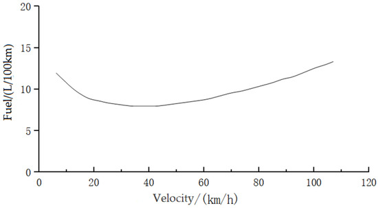 Figure 1. Relationship between vehicle speed and fuel consumption (Medium light vehicle).
Referring to the references [47], the relationship between fuel consumption and vehicle speed of different models listed in Table 2 is obtained.
Table 2.
The relationship between fuel consumption and vehicle speed of different models.
According to the available literature, the relationship between vehicle fuel consumption per unit distance and cargo capacity is linear when road conditions, driving techniques, vehicle speed, and other relevant factors are kept constant [48]. Its linear function can be expressed by the following equation.
where is the fuel consumption at full load. is the fuel consumption when unladen. is the amount of cargo carried by the transport vehicle. is the amount of full load of the transport vehicle.
In summary, the CO2 emissions are calculated based on the vehicle fuel consumption in the transportation and distribution process, and the expression is calculated as:
where is the carbon emissions from fuel consumption. is the fuel consumption of the vehicle. is the carbon dioxide emission factor. CO2 emission factors for different fuel types [49] are shown in Table 3.
Table 3.
CO2 emission factors for different fuel types.
According to China Carbon Trading Network, CO2 emission factor = average low-level heat generation * carbon content per unit calorific value * carbon oxidation rate * 44/12. By calculation, it can be concluded that the carbon emissions of ordinary trucks mentioned in this article are 22.3 kg per 100 km.
3.2.3. Satisfaction Analysis
In this article, we use a linear continuous time satisfaction function under a vehicle service time window to quantify customer time satisfaction (), and in practical applications, customers not only receive dispatch within the desired time window In practical applications, in addition to accepting dispatch within the desired time window, customers can also accept early or delayed arrival of vehicles for a period of time, which constitutes a maximum time window range However, customer satisfaction will gradually decrease with the early or late arrival of vehicles [50]. Assuming that customer time satisfaction is a linear function, as shown in Figure 2.
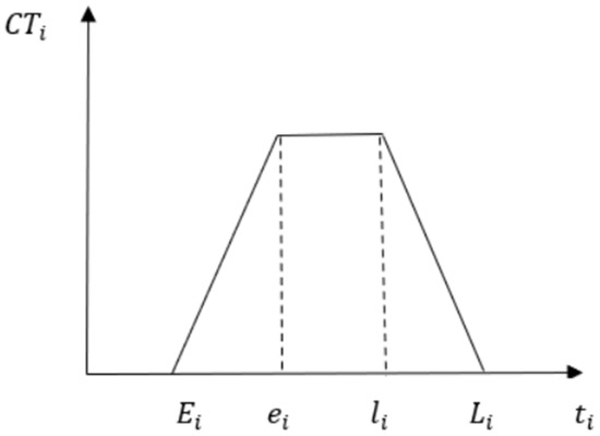
Figure 2.
Customer time satisfaction.
The expression of the customer time satisfaction function is as follows.
3.3. Model Building
In this article, the total costs and carbon emissions are minimized as the optimization objective, and the vehicle’s distribution route optimization model is established with time, satisfaction, and carrying capacity as constraints. In summary, the following is the objective function of the low-carbon vehicles distribution route optimization model for community group buying is as follows.
The constraints are:
Constraint (9) represents the objective function; Constraint (10) indicates that the cumulative driving time of the driver must not exceed the fatigue driving time; Constraint (11) indicates that the service time is within the specified time; Constraint (12) indicates that the average satisfaction for customer demand cannot be lower than the maximum satisfaction; Constraints (13) and (14) indicate that each demand point is served by only one vehicle and only once; Constraint (15) indicates the number of vehicles reserved, and trucks, assigned ; Constraint (16) indicates that the number of called distribution vehicles shall not exceed the number of vehicles owned by the distribution center; Constraint (17) indicates that each vehicle starts from the distribution center and finally returns to the distribution center; Constraint (18) indicates that the total amount of customer demand on the distribution route is not greater than the maximum capacity of the distribution vehicle; Constraint (19) indicates that the total route distance traveled by the distribution vehicle in the distribution process is not greater than the maximum driving mileage; Constraint (20) indicates that the speed of each distribution vehicle in the distribution process is not greater than the fastest driving speed of the vehicle; Constraints (21) and (22) are the decision variable functions.
4. Weight Calculation and Design of Improved Genetic Algorithm for Multi-Objective Distribution Route Problem
4.1. Weight Calculation
This article involves the calculation of multiple objective functions, and the weight calculation adopts a calculation method combining the analytic hierarchy method (AHP) and entropy weight method (EW), namely AHP-EW method; the steps are:
- (1)
- Starting from the economic and social benefits of the distribution center in Wu’an Town, a hierarchical model is established, with multi-objective optimization processing as Target layer A, and multi-objective factors as Criterion layer B, including economic benefits ( ), social benefits (), and cost () and carbon emissions () at the Scheme layer.
- (2)
- The middle and senior management of the distribution center scores the indicators and determines the judgment matrix, as shown in Table 4, Table 5 and Table 6, and obtains the weights of layer B relative to layer A and layer C relative to layer B, respectively.
Table 4. Matrix relationship between layer B and layer A.
Table 5. Matrix relationship between layer C and layer .
Table 6. Matrix relationship between layer C and layer .
It is calculated that CR(A) = 0, CR() = 0, and CR() = 0, so the consistency test holds. Furthermore, the weights of layer B relative to layer A are 0.76 and 0.24, and the weights of layer C relative to layer are 0.67 and 0.33, and the weights of layer C relative to layer are 0.33 and 0.67, respectively, so the cost weight is calculated as 0.5884, and the weight of carbon emissions is 0.4116, and the target weight is calculated by the entropy weight method. Through the survey of middle and senior managers, the comprehensive scoring results of each indicator are shown in Table 7. Thus, the initial matrix is obtained First, the data are dimensionless to obtain a matrix Then calculate the entropy , the entropy weight is . Therefore, the comprehensive weight of cost is 0.115, and the comprehensive weight of carbon emissions is 0.885.
Table 7.
Composite scores for each indicator.
- (3)
- The AHP-EW fusion technology is used to calculate the weight, and the comprehensive weight is obtained: the cost weight is 0.16, and the carbon emissions weight is 0.84.
4.2. Improved Algorithm Procedure
- (1)
- Chromosome Encoding
In the genetic algorithm, the fitness function indicates the superiority of chromosomes, so this article uses the genetic algorithm to solve the problem of the community group buying vehicle distribution route and uses a concise coding method to encode chromosomes [51]. However, the above encoding method cannot guarantee that all the decoded distribution routes meet the load constraint and time window constraint, and in order to solve the problem of violation of constraint, the penalty function is used as the constraint condition to solve.
- (2)
- Adaptation Function Design
The selection of the fitness function directly affects the convergence speed of the genetic algorithm, and the fitness function is established to find the excellent chromosome [52]. The larger the value of the fitness function, the better the fitness, representing the better the chromosome; that is, the greater the probability that the distribution solution will be selected in the actual problem to be solved.
Considering that the problem has a soft time window property, the fitness function for the problem should be
- (3)
- Introduce a Climbing Operator
The hill-climbing operator is a hill-climbing algorithm executed once for individuals in a subpopulation based on a certain probability before the subpopulation executes the genetic algorithm. Furthermore, the golden partition based on the contraction interval needs to be introduced during the execution of the hill-climbing algorithm [53]. Therefore, this article assumes that the initial population search interval is , denotes the population, denotes the population with dimension and is the contraction interval ratio, is the population size, and denotes the initial population dimension. The new search interval is solved as follows.
The mathematical definition of the climbing operator is as follows: assume that the population is
Step 1:;
Step 2: Based on the search interval of the previous body and the shrinkage ratio , to determine the new contraction range ;
Step 3: Perform the golden mean (0.618 method) for each individual in the population in the corresponding search interval, thus finding a new contraction interval on a new, better individual;
Step 4: Replace the old population with a population consisting of the resulting new individuals and perform the the operation;
Step 5: If , then return to step 2; otherwise, the algorithm stops executing.
- (4)
- Selection, Crossover, and Variation Operator Operations
According to the principle of traditional genetic algorithm, the selection operation uses the roulette wheel selection method; although this method is practical, it is prone to the premature phenomenon that as the number of iterations increases, the proportion of individuals with high fitness becomes larger and larger, falling into the local optimum, and thus cannot continue to search for the global optimal solution [54]. In studying the route planning problem, the natural number encoding is used, so the crossover process is improved with the variation process by having the chromosomes of n individuals undergo a transformation operation so that even if the individuals are all genetically identical, they can continue to reproduce iteratively until the global optimal solution is found. The transformation process means that the random gene segments of each group of n/m individuals selected are subjected to the inversion operation, a certain two random gene positions are subjected to the swap operation, and the random positions of genes are subjected to the flip operation twice, and the probability of transformation is set to [55].
- (5)
- Local Search Operation
The local search operation adopts the idea of destruction and recovery in a large-scale neighborhood search algorithm (LNS), that is, using the destruction operator to delete several customers in the current solution and then inserting the deleted customers back into the damaged solution through the recovery operator [56]. According to the similarity calculation formula, several customers with the same number are removed. On the premise of meeting the constraints of bearing capacity and time window, the removed customers are inserted back into the position where the total driving distance of the vehicle is minimized. The specific operation is as follows.
Symbol indicates the current solution; denotes the removed client, denotes the set of removed clients, denotes the number of removed clients, and denotes the number of clients removed from from the remaining part of the solution after the removal of customers. The specific procedure is as follows.
First, randomly take the customers from the set to as the set the first element of the set. The rest of the elements are selected as follows: one at a time from the set one customer is randomly selected from the set and the rest of the customers are arranged in the order of relevance from smallest to largest. From , the customers with the are selected, the most relevant customer is , and from select and add them to and repeat the process times until the remaining elements [57]. The correlation is defined as follows.
where denotes the value that will be the standardized value between [0, 1] and express and Euclidean distance.
indicates with whether they are on the same route and whether they are served by the same vehicle. It is 0 when on the same route and 1 otherwise. However, there is no perfect correlation function in real situations. If too much reliance is placed on the choice of the correlation function, various situations may arise for the eliminated customers. In order to avoid this situation, a random element is added to the algorithm. Namely its result is a customer in the correlation size sequence, that is, the hypothesis in accordance with the . The order of association is from largest to smallest, and the sorted sequence is then the result of the above process is []. It is concluded that when is 1, the removed customers are chosen completely randomly, and approaching positive infinity, the closer to the customer with the greatest association. The larger the value is, the more favorable the customers with large associations. In this article, we use the improved genetic algorithm to make up for the deficiencies, such as premature convergence of the traditional genetic algorithm, increase the local search ability, and then derive the best distribution route. The algorithm procedure is shown in Figure 3.
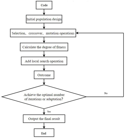
Figure 3.
Improved algorithm procedure.
5. Empirical Analysis
5.1. Data Sources
Wu’an Town, Wu’an City, Hebei Province, with a jurisdiction area of 41.5 square kilometers and a permanent population of about 200,000, is located in the east-central part of Wu’an City. Wu’an Town Community Group Buying Distribution Center sales categories are mainly fruits and vegetables, fresh food, rice flour, oil grain, and services, once a day to the surrounding 14 township customer points to deliver goods, vehicles unified from the distribution center, assuming that the time to the first customer is customer satisfaction of one time, then the route needs to meet the time window requirements, so as to obtain the best number of vehicles used and the optimal distribution route, the specific relevant parameters are shown in Table 8, the location of 14 township distribution points is shown in Figure 4.
Table 8.
Distribution Center and Customer Point Information Sheets.
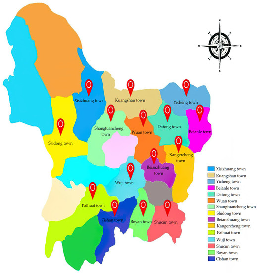
Figure 4.
The location of 14 township distribution points in Wu’an town.
5.2. Parameter Setting
In order to verify the effectiveness of the algorithm designed in this article, the traditional genetic algorithm, the traditional ant colony algorithm, and the improved genetic algorithm are compared. Let the distribution center number be 0, have five trains of the same type, the load capacity of the truck is 3000 kg, the transportation cost is 0.86 RMB/km, the fixed cost is 300 RMB/day, the average speed of the vehicle is 60 km/h, the carbon emissions are 0.223 kg/km, and the penalty cost is 1.5.
5.3. Model Application
Through the Matlab programming simulation operation, the route in the study has been optimized by using the traditional genetic algorithm, the traditional ant colony algorithm, and the improved genetic algorithm, and the results and effects of the model after optimization processing by three different algorithms are shown in Figure 5, Figure 6 and Figure 7.
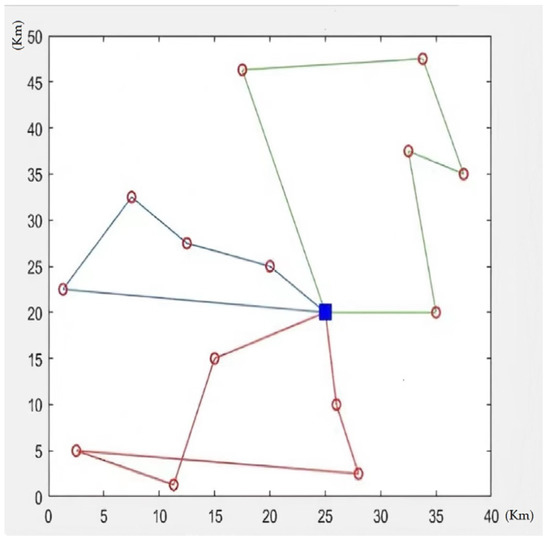
Figure 5.
Traditional genetic algorithm distribution route.
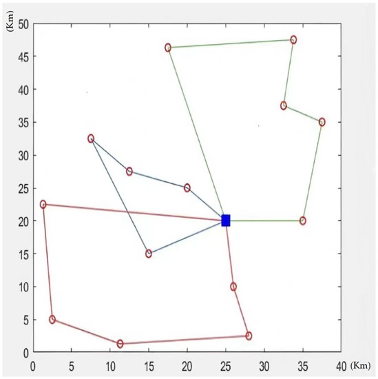
Figure 6.
Traditional ant colony algorithm distribution route.
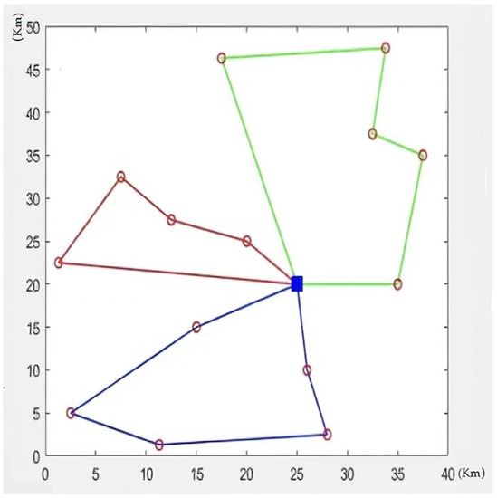
Figure 7.
Improved genetic algorithm distribution route.
After 1000 iterations, the total target optimization fitness obtained by the three optimization algorithms is shown in Figure 8. In the process of 1000 iterations, the improved genetic algorithm always has the lowest adaptation value and the highest optimization quality, which effectively avoids the blind search at the beginning of the iteration and the problem of excessive search time and local optimization of the simple algorithm, and obtains a high-quality solution for the optimization of the distribution route of the community group buying logistics. The improved genetic algorithm has strong global optimization ability, and the total costs and carbon emissions are the lowest based on considering time, penalty cost, and customer satisfaction. The distribution routing scheme determined in this way enables just-in-time delivery, which improves the quality of delivery services.
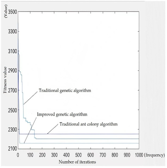
Figure 8.
Comparison of fitness values of three algorithms.
5.4. Analysis of Optimization Results
A comparison of the calculated results of the three algorithms is shown in Table 9.
Table 9.
Comparison of calculation results.
It can be seen from Table 9 that under the premise of meeting customer needs, by comparing the mileage of the three distribution routes, the distribution route determined by the improved genetic algorithm is reduced by 9.57% compared with the other two algorithms, and the total costs are reduced by 1.62% compared with the traditional genetic algorithm. Compared with the traditional ant colony algorithm, the carbon emissions are reduced by 5.84%, and the total costs are reduced by 1%. It can be seen that optimizing the distribution scheme of distribution vehicles and reducing the total distance of vehicle distribution can directly reduce carbon emissions and fuel consumption costs, which is of positive significance for reducing the total costs of enterprises and improving their efficiency.
6. Conclusions
Under the dual-carbon goal, there are many distribution modes for community group buying, but no matter what kind of logistics distribution mode is chosen, having a high-efficiency and low-cost vehicles distribution route is not only in line with the theme of the times but also an important factor for enterprises to gain a place in the fierce competition and long-term development. Under the premise of taking into account economic benefits and environmental benefits, this article is based on actual considerations; for the problem of community group buying and distribution, the best scheme of vehicle scheduling is found by using improved genetic algorithms so as to shorten the total distance of the logistics and distribution process, reduce carbon emissions, total costs, and air pollution, and take the road of combining with nature.
- (1)
- In terms of algorithm improvement, this article models and analyzes the distribution problem in community group buying, studies the solution principle of traditional genetic algorithm, introduces mountain climbing operators, improves the crossover and mutation process in traditional genetic algorithm, adopts the idea of destruction and recovery in large-scale neighborhood search algorithm (LNS), improves local search ability, and verifies that the model can effectively improve distribution efficiency, reduce the costs and carbon emissions generated during distribution.
- (2)
- In terms of model improvement, comprehensively considering the total costs of distribution and carbon emissions as the optimization goals, the analytic hierarchy method (AHP) and entropy weight method (EW) were used to calculate the carbon emissions and cost weights, and five main costs were analyzed according to the characteristics of community group buying distribution routes, under the constraints of delivery time and customer satisfaction. Then the improved genetic algorithm was designed to solve them, and the effectiveness of the proposed model and the advantages of the improved algorithm were verified by examples.
- (3)
- In terms of optimization results, taking the 14 township customer points served by the community group buying distribution center in Wu’an Town, Hebei Province, as an example, without changing the number of dispatched vehicles, the improved genetic algorithm is better than the other two algorithms in terms of convergence and optimal solution, and the quality of the results was higher, indicating the use value of the algorithm and model and the effectiveness of reducing carbon emissions.
In this article, the optimization of vehicle distribution routes under the community group buying mode is studied, and although certain research results have been achieved, there are still some limitations due to the complexity of vehicle route optimization problems, and further research is needed in the future. Due to the current logistics distribution using fuel vehicles, the limitation of this article is the distribution business only considers fuel vehicles, but in the actual situation, more and more logistics companies distribute goods by fuel vehicles and electric logistics vehicles to complete together, this article does not involve the mixing of the two. In the future, a comprehensive and in-depth study can be carried out on the vehicle routing optimization problem of the joint distribution of fuel vehicles and electric vehicles.
In the route optimization problem, considering carbon emissions and total costs of distribution is a worthy research problem, which helps to reduce the energy consumption of the whole transportation. In today’s booming e-commerce, this method can be extended to more logistics fields through continuous improvement in the future, which has positive significance to further reduce the carbon emissions of the whole logistics industry and improve the economic efficiency of enterprises. At the same time, it responds to China’s concept of low-carbon environmental protection and promotes the transformation of the world economy to a green economy and sustainable economic situation.
Author Contributions
Conceptualization, Z.L. and C.G.; data curation, Y.N.; formal analysis, S.J.; investigation, Y.N.; methodology, Y.N.; supervision, Z.L.; validation, S.J.; writing-original draft, Y.N. and Z.L.; writing-review and editing, C.G. and S.J. All authors have read and agreed to the published version of the manuscript.
Funding
This research received no external funding.
Institutional Review Board Statement
Not applicable.
Informed Consent Statement
Not applicable.
Data Availability Statement
Data are available upon request from the corresponding author.
Conflicts of Interest
The authors declare no conflict of interest.
References
- Song, W.; Yuan, S.; Yang, Y.; He, C. A Study of Community Group Purchasing Vehicle Routing Problems Considering Service Time Windows. Sustainability 2022, 14, 6968. [Google Scholar] [CrossRef]
- Li, L.L. Research on the Development of Community Group Buying Based on the Perspective of New Retail. Mod. Mark. (First Issue) 2022, 12, 88–90. [Google Scholar]
- Baradaran, V.; Shafaei, A.; Hosseinian, A.H. Stochastic vehicle routing problem with heterogeneous vehicles and multiple prioritized time windows: Mathematical modeling and solution approach. Comput. Ind. Eng. 2019, 131, 187–199. [Google Scholar] [CrossRef]
- Keskin, M.; Catay, B. A matheuristic method for the electric vehicle routing problem with time windows and fast chargers. Comput. Oper. Res. 2018, 100, 172. [Google Scholar] [CrossRef]
- Ghoseiri, K.; Ghannadpour, S.F. Multi-objective vehicle routing problem with time windows using goal programming and genetic algorithm. Appl. Soft Comput. 2010, 10, 1096–1107. [Google Scholar] [CrossRef]
- Zhang, H.; Zhang, Q.; Ma, L.; Zhang, Z.; Liu, Y. A hybrid ant colony optimization algorithm for a multi-objective vehicle routing problem with flexible time windows. Inf. Sci. 2019, 490, 166–190. [Google Scholar] [CrossRef]
- Nobre, A.V.; Oliveira, C.C.R.; de Lucena Nunes, D.R.; Silva Melo, A.C.; Guimarães, G.E.; Anholon, R.; Martins, V.W.B. Analysis of Decision Parameters for Route Plans and Their Importance for Sustainability: An Exploratory Study Using the TOPSIS Technique. Logistics 2022, 6, 32. [Google Scholar] [CrossRef]
- Lai, P.Z.; Tang, Y.; Yang, Z.H.; Jin, Z.H. Distribution optimization considering traffic control of urban freight vehicles. J. Dalian Marit. Univ. 2015, 41, 59–66. [Google Scholar]
- Xiao, J.H.; Wang, C.W.; Chen, P.; Niu, Y.Y. Multi-energy multi-vehicle route optimization based on urban road control. Syst. Eng. Theory Pract. 2017, 37, 1339–1348. [Google Scholar]
- Li, J.; Ren, L.; Sun, M. Is There a Spatial Heterogeneous Effect of Willingness to Pay for Ecological Consumption? An Environ-mental Cognitive Perspective. J. Clean. Prod. 2020, 245, 118259. [Google Scholar] [CrossRef]
- Liu, L.; Zhang, F.; Li, H.; Wen, C. Research on the Community Group Buying Marketing Model of Fresh Agricultural Products in Jilin Province from the Perspective of Internet Marketing and Retail. IOP Conf. Ser. Earth Environ. Sci. 2021, 769, 022054. [Google Scholar] [CrossRef]
- Peng, B.T. Challenges and countermeasures of community group buying mode under the background of new retail. Shopp. Mall Mod. 2020, 914, 65–67. [Google Scholar]
- Jing, R.; Yu, Y.; Lin, Z. How Service-Related Factors Affect the Survival of B2T Providers: A Sentiment Analysis Approach. J. Organ. Comput. Electron. Commer. 2015, 25, 316–336. [Google Scholar] [CrossRef]
- Hsu, M.H.; Chuang, L.W.; Hsu, C.S. Understanding Online Shopping Intention: The Roles of Four Types of Trust and Their Antecedents. Internet Res. 2014, 24, 332–352. [Google Scholar] [CrossRef]
- McKinnon, A.C. Product-level carbon auditing of supply chains. Int. J. Phys. Distrib. Logist. Manag. 2010, 40, 42–60. [Google Scholar] [CrossRef]
- Hoen, K.M.R.; Tan, T.; Fransoo, J.C.; Houtum, G.J. Effect of carbon emissions regulations on transport mode selection under stochastic demand. Flex. Serv. Manuf. J. 2014, 26, 170–195. [Google Scholar] [CrossRef]
- Tacken, J.; Rodrigues, V.S.; Mason, R. Examining CO2e reduction within the German logistics sector. Int. J. Logist. Manag. 2014, 25, 54–84. [Google Scholar] [CrossRef]
- Li, J.; Zhang, J.H. Research on the Influence of Carbon Trading Mechanism on Logistics Distribution Path Decision. Syst. Eng. Theory Pract. 2014, 7, 1779–1787. [Google Scholar]
- Leng, L.; Zhang, J.; Zhang, C.; Zhao, Y.; Wang, W.; Li, G. A novel bi-objective model of cold chain logistics considering location-routing decision and environmental effects. PLoS ONE 2020, 15, e0230867. [Google Scholar] [CrossRef]
- Tao, D.H.; Liu, R.; Lei, Y.J.; Zhang, Q.X. Cold chain logistics distribution path optimization based on green supply chain. Ind. Eng. 2019, 22, 89–95. [Google Scholar]
- da Costa PR, D.O.; Mauceri, S.; Carroll, P.; Pallonetto, F. A Genetic Algorithm for a Green Vehicle Routing Problem. Electron. Notes Discret. Math. 2018, 64, 65–74. [Google Scholar] [CrossRef]
- Ghane, E.M.; Vergara, H.A. Decomposition approach for integrated intermodal logistics network design. Transp. Res. Part E Logist. Transp. Rev. 2016, 89, 53–69. [Google Scholar] [CrossRef]
- Agatz, N.; Campbell, A.M.; Fleischmann, M. Challenges and Opportunities in Attended Home Delivery. Oper. Res./Comput. Sci. Interfaces Ser. 2007, 43, 28. [Google Scholar]
- Ren, T.; Chen, Y.; Xiang, Y.C.; Xing, L.N.; Li, S.D. Low carbon cold chain vehicle routing optimization considering customer satisfaction. Comput. Integr. Manuf. Syst. 2020, 26, 1108–1117. [Google Scholar]
- Tao, Z.W.; Zhang, Z.Y.; Shi, Y.; Zhang, Y.W.; Shi, Y.Q. Multi-objective cold chain logistics distribution path optimization under carbon tax system. J. Wuhan Univ. Technol. (Inf. Manag. Eng. Ed.) 2019, 41, 51–56. [Google Scholar]
- Turkenstein, M. The accuracy of carbon emissions and fuel consumption computations in green vehicle routing. Eur. J. Oper. Res. 2017, 262, 647–659. [Google Scholar] [CrossRef]
- Mak, S.L.; Wong, Y.M.; Ho, K.C.; Lee, C.C. Contemporary Green Solutions for the Logistics and Transportation Industry—With Case Illustration of a Leading Global 3PL Based in Hong Kong. Sustainability 2022, 14, 8777. [Google Scholar] [CrossRef]
- Ziółkowski, J.; Lęgas, A.; Szymczyk, E.; Małachowski, J.; Oszczypała, M.; Szkutnik-Rogoż, J. Optimization of the Delivery Time within the Distribution Network, Taking into Account Fuel Consumption and the Level of Carbon Dioxide Emissions into the Atmosphere. Energies 2022, 15, 5198. [Google Scholar] [CrossRef]
- Dantzig, G.; Ramser, J. The Truck Dispatching Problem. Manag. Sci. 1958, 6, 80–91. [Google Scholar] [CrossRef]
- Fan, J. The Vehicle Routing Problem with Simultaneous Pickup and Delivery Based on Customer Satisfaction. Procedia Eng. 2011, 15, 5284–5289. [Google Scholar] [CrossRef]
- Guerriero, F.; Surace, R.; Loscri, V.; Natalizio, E. A Multi-objective Approach for Unmanned Aerial Vehicle Routing Problem with Soft Time Windows Constraints. Appl. Math. Model. 2014, 38, 839–852. [Google Scholar] [CrossRef]
- Jin, S.T.; Lv, S.; Wu, Y.M.; Wang, Y.Y. Research on Logistics Distribution Path Optimization Method Based on Improved Genetic Algorithm. Comput. Digit. Eng. 2017, 45, 629–631. [Google Scholar]
- Baker, B.M.; Ayechew, M.A. A genetic algorithm for the vehicle routing problem. Comput. Oper. Res. 2003, 30, 787–800. [Google Scholar] [CrossRef]
- Paksoy, T.; Pehlivan, N.Y.; Özceylan, E. Application of fuzzy optimization to a supply chain network design: Case study of an edible vegetable oils manufacturer. Appl. Math. Model. 2012, 36, 2762–2776. [Google Scholar] [CrossRef]
- Sahar, V.; Arijit, B.; Byrne, P.J. A case analysis of a sustainable food supply chain distribution system—A multi-objective approach. Int. J. Prod. Econ. 2014, 152, 71–87. [Google Scholar]
- Teimoury, E.; Nedaei, H.; Ansari, S.; Sabbaghi, M. A multi-objective analysis for import quota policy making in a perishable fruit and vegetable supply chain: A system dynamics approach. Comput. Electron. Agric. 2013, 93, 37–45. [Google Scholar] [CrossRef]
- Liu, S.; Papageorgiou, L.G. Multi-objective optimization of production, distribution and capacity planning of global supply chains in the process industry. Omega. 2013, 41, 369–382. [Google Scholar] [CrossRef]
- Özceylan, E.; Paksoy, T. Fuzzy multi-objective linear programming approach for optimizing a closed-loop supply chain network. Int. J. Prod. Res. 2013, 51, 2443–2461. [Google Scholar] [CrossRef]
- Bozorgi, A.; Pazour, J.; Nazzal, D. A new inventory model for cold items that considers costs and emissions. Int. J. Prod. Econ. 2014, 155, 114–125. [Google Scholar] [CrossRef]
- Bortolini, M.; Faccio, M.; Ferrari, E.; Gamberi, M.; Pilati, F. Fresh food sustainable distribution: Cost, delivery time and carbon footprint three-objective optimization. J. Food Eng. 2016, 174, 56–67. [Google Scholar] [CrossRef]
- Jaramillo, J.H.; Bhadury, J.; Batta, R. On the use of genetic algorithms to solve location problems. Comput. Oper. Res. 2002, 29, 761–779. [Google Scholar] [CrossRef]
- Syarif, A.; Yun, Y.; Gen, M. Study on multi-stage logistic chain network: A spanning tree-based genetic algorithm approach. Comput. Ind. Eng. 2002, 43, 299–314. [Google Scholar] [CrossRef]
- Wee-kit; Ahbrid. Serach Algorithm for The Vehicle Routing Problem with Time Windows. Int. J. Artif. Intell. Tools 2001, 3, 431–449. [Google Scholar]
- Hsiao, Y.H.; Chen, M.C.; Lu, K.Y.; Chin, C.L. Last-mile distribution planning for fruit-and-vegetable cold chains. Int. J. Logist. Manag. 2018, 29, 862–886. [Google Scholar] [CrossRef]
- Dias Santos, J.; Marques, F.; Garcés Negrete, L.P.; Andrêa Brigatto Gelson, A.; LópezLezama, J.M.; MuñozGaleano, N. A Novel Solution Method for the Distribution Network Reconfiguration Problem Based on a Search Mechanism Enhancement of the Improved Harmony Search Algorithm. Energies 2022, 15, 2083. [Google Scholar] [CrossRef]
- Wan, Y. Research on the optimization of distribution path of fresh agricultural products from a low-carbon perspective[D]. Kunming Univ. Sci. Technol. 2021, 1, 61. [Google Scholar]
- Zhou, Y.F.; Zhang, H.R. Research on the relationship between pavement surface characteristics and automobile fuel consumption. Highway. 2005, 1, 30–36. [Google Scholar]
- Xiao, Y.; Zhao, Q.; Kaku, I.; Xu, Y. Development of a fuel consumption optimization model for the capacitated vehicle routing problem. Comput. Oper. Res. 2012, 39, 1419–1431. [Google Scholar] [CrossRef]
- Kang, K.; Han, J.; Pu, W.; Ma, Y.F. Study on Optimization of low-carbon Distribution Route of cold chain logistics of fresh agricultural products. Comput. Eng. Appl. 2019, 55, 259–265. [Google Scholar]
- Cao, Q.; Shao, J.P.; Sun, Y.A. Multi-objective distribution path optimization of fresh agricultural products based on improved genetic algorithm. Ind. Eng. 2015, 18, 71–76. [Google Scholar]
- Pan, J.; Wang, X.S.; Cheng, Y.H. Mobile robot path planning based on improved ant colony algorithm. J. China Univ. Min. Technol. 2012, 1, 108–113. [Google Scholar]
- Xu, J.X.; Liu, W. Improved genetic algorithm based on climbing operator and fitness sharing. J. Guangdong Univ. Technol. 2011, 1, 78–81. [Google Scholar]
- Guo, H.P. Research on logistics distribution path optimization based on improved genetic algorithm. Xidian Univ. 2015, 3, 71. [Google Scholar]
- Liu, N.C.; Zhang, L.Y.; Yang, Y.Y.; Qiu, R.Z. Vehicle Sales Logistics Distribution Route Optimization Based on Genetic Algorithm. Math. Pract. Underst. 2021, 7, 35–42. [Google Scholar]
- Wang, X.P.; Zhan, H.X.; Sun, Z.L.; Li, F.F. Product oil multi-cabin delivery path optimization with replenishment time window. Manag. Eng. J. 2020, 34, 182–195. [Google Scholar]
- Peng, B.T.; Zhou, S.P. Vehicle routing problem with three-dimensional loading constraints. Comput. Eng. Appl. 2016, 52, 242–247. [Google Scholar]
- Zhang, H.Y.; Hu, R.; Qian, B. Hyper-heuristic Estimation of Distribution Algorithm for Simultaneous Pickup and Delivery Vehicle Routing Problem with Soft Time Window. Control Theory Appl. 2021, 38, 1427–1441. [Google Scholar]


Disclaimer/Publisher’s Note: The statements, opinions and data contained in all publications are solely those of the individual author(s) and contributor(s) and not of MDPI and/or the editor(s). MDPI and/or the editor(s) disclaim responsibility for any injury to people or property resulting from any ideas, methods, instructions or products referred to in the content. |
© 2023 by the authors. Licensee MDPI, Basel, Switzerland. This article is an open access article distributed under the terms and conditions of the Creative Commons Attribution (CC BY) license (https://creativecommons.org/licenses/by/4.0/).