Abstract
Biomass gasification has obtained great interest over the last few decades as an effective and trustable technology to produce energy and fuels with net-zero carbon emissions. Moreover, using biomass waste as feedstock enables the recycling of organic wastes and contributing to circular economy goals, thus reducing the environmental impacts of waste management. Even though many studies have already been carried out, this kind of process must still be investigated and optimized, with the final aim of developing industrial plants for different applications, from hydrogen production to net-negative emission strategies. Modeling and development of process simulations became an important tool to investigate the chemical and physical behavior of plants, allowing raw optimization of the process and defining heat and material balances of plants, as well as defining optimal geometrical parameters with cost- and time-effective approaches. The present review paper focuses on the main literature models developed until now to describe the biomass gasification process, and in particular on kinetic models, thermodynamic models, and computational fluid dynamic models. The aim of this study is to point out the strengths and the weakness of those models, comparing them and indicating in which situation it is better to use one approach instead of another. Moreover, theoretical shortcut models and software simulations not explicitly addressed by prior reviews are taken into account. For researchers and designers, this review provides a detailed methodology characterization as a guide to develop innovative studies or projects.
1. Introduction
During the Anthropocene, pressure on the environment has been increasing exponentially along with global warming. The need for each country to be energy-independent and to find low-price solutions for energy production represent a real challenge.
In order to deal with those problems, many researchers pointed out that it is possible to make an energetic transition from fossil fuels to renewable energy sources. Among the most investigated renewable energy sources, biomass is confirmed as the most favorable one, since it is the widest source of energy after coal, oil, and natural gas [1,2,3,4]. Using biomass as feedstock for energy production allows achieving both green energy production and national energy security goals. Moreover, using biomass waste instead of energetic culture accomplish the goal of a circular economy in reusing those organic wastes that otherwise would be disposed of, polluting soil and air, and also avoiding the fuel vs. food issue [5,6,7].
During the last few years, many processes for biomass conversion into energy were investigated, and gasification was highlighted as one of the most efficacious [8,9,10]. Gasification is a thermochemical technology to convert biomass into a combustible gas mixture by the partial oxidation of the biomass at high temperature (750–950 °C) in the presence of a gasifying agent [11,12,13,14]. The fluidized bed reactor was confirmed as the most suitable as gasifier reactor due to the excellent thermal and mixing properties that ensure high heat transfer rates, high efficiency, low combustion temperature and low pollutant emissions [15,16]. The gas mixture produced by gasification process is called syngas and it is mainly made of H2, CO, CO2, CH4, H2O, along with organic and inorganic contaminants [17]. The quantity of each produced component depends on feedstock characteristics, gasifying agent, operative conditions of the process, reactor design, etc.
To investigate the biomass waste gasification process, modeling approaches and simulation software provide useful tools to investigate different operative conditions to achieve a first raw optimization of the process, obtaining the most suitable syngas for the desired uses and scaling up of lab-scale and pilot apparatus. Results coming from simulative models must be the base for the realization of a pilot plant, allowing for reduced cost, avoiding risk to human health, interpreting the experimental data, and building the foundations of knowledge necessary for the realization of a project [18]. Both mathematical and numerical simulative models are suitable for those purposes, since they are both able to predict the performance of the process and to give an adequate description of the chemical and physical phenomena occurring, in order to optimize the process swiftly and with minimal cost [19]. Then, it is also possible to choose to simulate the process in a steady-state condition (time independent) or in a dynamic condition (time-dependent), according to what the focus of the investigation is. Kinetic, thermodynamic, computational fluid dynamic (CFD), and artificial neural network (ANN) models have been adapted and implemented for the study of syngas production from a wide variety of feedstocks [20,21,22,23].
Kinetic models take into account the kinetics of the gasification reactions given the reactor properties (residence time, operative temperature, and pressure). They predict the syngas yield and the syngas composition produced after a finite time or in a finite volume in a flowing medium. These models, after proper validation, allow us to predict the process performances for a specific operating conditions and reactor design [24,25].
Since kinetic models depend on the specific fluid dynamics and geometry of the case study, their applicability is restricted to specific reactor configurations. Complex configurations of reactors enhance the complexity of the descriptive model.
Thermodynamic models predict the syngas composition based on the assumption that the reactants react in a fully mixed condition for an infinite time so to reach the thermodynamic equilibrium [26]. The main advantage of those models is their independence from the gasifier design [27], which means that thermodynamic models can be used to describe a wide range of plants without any particular restrictions, despite kinetic models.
CFD models describe the gasification process based on the conservation of mass, momentum, species, and energy into a certain portion [26,28]. Those models are able to predict a very accurate syngas composition when coupled with a well-known fluid dynamic of the gasifier and are especially suitable for fluidized bed reactors, in which they provide important information about temperature profiles and species concentration.
Black-box approaches, including algorithms of artificial intelligence such as ANN, are considered a relatively new approach for modeling the biomass gasification process. They have the great merit of not requiring the formulation of complex mathematical equations and also to be able to understand and identify non-linear relations [29]. Therefore, ANN modeling is attracting great interest when the aim of the study is to investigate biomass gasification process. There are complex non-linearities occurring in the dataset [30].
First of all, the authors of the present paper investigated the status of biomass gasification modeling in the literature and selected some of the most relevant review papers [22,31,32,33]. The authors noticed that there had not been a comprehensive study taking into account and discussing kinetic, thermodynamic, CFD, multivariate data analysis (MVDA) and ANN. Most literature reviews are all about kinetic, thermodynamics and CFD, very few are about ANN, and almost none about MVDA. Moreover, in the literature, there is not a single review that takes into account the Gibbs free-energy gradient method model within the thermodynamic model. As such, the aim of the present paper is to investigate the most recent simulative models and results from scientific literature, in order to fill the lack present in the literature and to provide a critical review that is able to indicate which is the best approach among kinetics, thermodynamic, CFD, multivariate data analysis (MVDA) and ANN to describe a biomass gasification process according to the specifications and the desired goal.
2. Biomass Gasification Principle and Technology
Gasification is a partial thermal oxidation occurring at high temperature (in the range 750–900 °C) in the presence of a gasifying agent (steam, air, oxygen, or a mixture of them) that reacts with biomass, producing a gaseous product mainly composed of H2, CO, CH4, and CO2 along with small quantities of solid product (char), inorganic contaminants (mainly H2S and HCl), and organic contaminants (tar). The amount of final inorganic compounds depends on biomass inlet properties, for instance, it is recommended that the inlet concentrations of S and Cl be as low as possible. The gasifying agent influences the final gas composition (see Table 1), steam provides the highest H2 content and the highest low heating value (LHV), while air provides a lower-quality syngas due to the higher content of inlet N2.

Table 1.
Effect of gasifying agents on the composition of gas products [23].
The chemistry of biomass gasification is rather complicated. The reactions involved in the process are listed in Table 2, and the gasification stages can be summarized as follows [34,35].
Table 2.
Chemical reactions of gasification process [34,36,37].
- ○
- Drying. Occurring at 100–200 °C, the drying stage reduces the moisture content of biomass below 5%.
- ○
- Devolatilization (pyrolysis). In this step, the thermal decomposition of biomass occurs in the absence of oxygen or air. The volatile matter is decreased, releasing hydrocarbon gases from biomass, and is then reduced to solid charcoal.
- ○
- Oxidation. In this stage, CO2 is produced from the reaction of solid carbonized biomass and oxygen in the air. H2 present in the biomass is oxidized to produce water. Then, if oxygen is present in sub-stoichiometric quantities, partial oxidation of carbon may happen, producing CO.
- ○
- Reduction. At high temperatures (800–950 °C) several reduction reactions occur in the absence (or sub-stoichiometric presence) of oxygen, i.e., water–gas reaction, Boudouard reaction, water–gas shift reaction, and methane reaction.
3. Thermodynamic Models
Thermodynamic models describe the thermodynamic equilibrium (temperature, pressure, and composition) achieved by perfect mixing and infinite reaction time. The system is time-invariant and not dependent on kinetic factors such as the design of reactor or fluid dynamics [27]. This property makes the models at thermodynamic equilibrium very flexible to use and suitable for a wide variety of processes without any specific constraints. Indeed, they provide information about limit gas yield and gas composition, and even if they apply under many rescripted assumptions, they still provide insights about unit operation, process optimization, energy recovery, and life-cycle assessment and techno-economic analysis [2,38,39,40]. Equilibrium models have a wide range of applicability, since usually the gasification process is driven close to equilibrium [27]. Thermodynamic equilibrium models can be classified into [31,41,42]:
- Stoichiometric models, which are based on equilibrium constants: the specific chemical reactions of the process must be declared;
- Non-stoichiometric models, which are based on minimization of Gibbs free energy, neglecting the chemical reactions involved. Only the definition of a set of chemical compounds that are expected at equilibrium is needed.
Gonzalez-Vazquez et al. [43] developed two models, one stoichiometric and one non-stoichiometric, for a fluidized-bed gasifier using pine kernel shells as biomass input. Syngas composition from both models, at 900 °C and S/B ratio 0.2, are shown in Figure 1 and compared with experimental data, in order to discuss the effectiveness of the models.

Figure 1.
Comparison of H2, CO and CO2 concentration at 900 °C and S/B 0.2 [43].
CO2 and CO concentrations from stoichiometric and non-stoichiometric models are similar and in good agreement with experimental data in the case of CO2, while lower than experimental data in the case of CO. The underprediction of CO is likely due to lower prediction of char-steam gasification in modeling, rather than the real plant. Then, both models present an overproduction of H2 compared to experimental data. This trend can be ascribed to the neglection of tar in modeling. Moreover, it can be noticed that the stoichiometric model offered more accuracy in hydrogen production, and this can be explained by the setting of each model. Indeed, when using the stoichiometric model, the authors defined only the most relevant gasification reactions, while in the non-stoichiometric model, the reaction mechanism is not included in the simulation. This observation can suggest that the stoichiometric model can be adjusted to come closer the experimental data by means of a proper selection of gasification reactions to be included in the model. Stoichiometric models and non-stoichiometric models, even if built using completely different mathematical implementation, were demonstrated to reach close results if some conditions were satisfied [44]. Even if stoichiometric models are based on simple mathematical formulation, they have not been widely utilized in the literature, while non-stoichiometric models are used in approximately 73% of equilibrium simulations in the literature, while 27% of the literature relies on stoichiometric ones [31].
Stoichiometric models include mass balances and the calculation of equilibrium constants at a given temperature. The mathematical model combines the conservation laws of atomic species with those of thermodynamic equilibrium by referring to the global gasification reaction, starting from reactants and inert compounds in the feed. The result is a tool to predict the composition of the produced gas once the characteristics of the feed to be gasified are known (proximate and ultimate analysis), such as the operating conditions in terms of pressure, temperature, and steam/feed ratio. Mass and energy balances result in a system of non-linear algebraic equations for each reaction whose unknown variables are the extent of each reaction. The solution is found by applying the classic methods to evaluate the roots of non-linear algebraic equations, such as the Newton–Rapson one. Once the extent of all reactions at equilibrium has been computed, it is possible to compute the equilibrium composition of the products at a given temperature. If the temperature is unknown, it is necessary to couple an energy balance taking into account the enthalpies of the reactants and products, thus increasing the complexity of the system. These models are commonly based on the following assumptions [45].
- (a)
- All the reactions considered are at thermodynamic equilibrium equivalent to an infinite residence time.
- (b)
- All the carbon is gasified and is not present among the reaction products.
- (c)
- The products leaving the gasifier, except for the ashes in the solid phase, are in the gaseous phase and consist of CO, CO2, H2O, H2, CH4, N2.
- (d)
- Among the reaction products, there is no tar.
The mass balances in the presence of the equilibrium reaction require the molar concentrations and the molar ratios of components in the feedstock. Since the solid feedstock (solid biomass) is often a complex mixture, it is described by a brute formula derived from the ultimate analysis of dry and ash-free biomass samples. Thus, the feedstock is represented as a single component, CHmOpNq, reacting as:
and are the variation in standard Gibbs free energy and enthalpy formation, respectively.
Assuming that the composition of the biomass and the characterization of the reactants are known, including the biomass moisture and the gasifying agent (steam), it is possible to develop the model taking into account two chemical reactions: water–gas shift (9) and steam reforming (10). The solving system is represented by the four mass balance equations and the two chemical equilibrium Equations (20)–(27).
1 = a + b + c
m + 2w = 2c + 4d + 2e
q = 2f
p + w = a + 2b + e
P0 represents the system operative pressure, PCH4, PH2, PH2O, and PCO2 are the partial pressures of CH4, H2, H2O, and CO2, respectively, and nT is the total moles of produced gas. In Table 3 are listed the values of standard Gibbs free energy and enthalpy formation.
Table 3.
Standard Gibbs free energy and molar enthalpy formation [45].
These models are of rapid use and are based on solid theoretical foundations widely developed in chemical engineering and reactor engineering textbooks. On the other hand, they often generate a non-negligible error due to the reactions really occurring being only partially known: they describe only the gaseous phase at a given fixed temperature where all reactions are in equilibrium.
Non-stoichiometric models demonstrated their reliability over the years since being successfully used in modeling the gasification process, especially in fluidized-bed gasifiers [41,46,47,48], allowing the evaluation of the effect of temperature, equivalence ratio, steam-to-biomass ratio, and moisture content of feedstock on the gasification process.
Non-stoichiometric equilibrium models may be upgraded to the so-called quasi-equilibrium approach, which is a compromise between equilibrium thermodynamic models and experimental data in reaction conditions close to the equilibrium [27,46], providing more accurate results about syngas composition.
The non-stoichiometric equilibrium modeling approach is founded on the direct minimization of the Gibbs free energy of reaction species. This methodology can be used to find equilibrium compositions “virtually,” including unknown reaction paths. On the other hand, the minimization of the Gibbs free energy can be stopped in non-equilibrium conditions, as explained in our previous works [45,47], and in some cases, this is referred to as the quasi-equilibrium temperature (QET) approach. This latter is actually considered the most effective way to model the gasification process [20] and has also been adopted by commercial process simulators, as mentioned in the next chapters. The final composition is derived by setting a QET for each reaction that occurs into the gasifier. In this way, each reaction occurs at its equilibrium temperature instead of the gasification temperature set for the gasifier block [48]. On the other hand, the minimization can be stopped by introducing other criteria. For instance, in our previous work [47], we defined an algorithm based on the minimization of the error model predictions and experimental data. In this way, it is possible to train a quasi-equilibrium model and then use it as a scaling-up tool. We report below the formulation of a non-stoichiometric model based on the minimization of Gibbs free energy (G) for the previously selected set of reactions: steam reforming and water–gas shift. It must be premised that this type of modeling starts following a first devolatilization defining the composition of the gaseous state that participates in the reaction. This preliminary phase is often trained on experimental data to get a more realistic description of the formation of ash, char, and tar. In fixed temperature and pressure conditions, the function G depends only on the extent of the reactions and , expressed as an extensive variable as follows:
where i = CO, CO2, H2O, H2, CH4, N2, H2S. The partial pressure Pi assumes an ideal mixture of gases, ni is the number of moles of the i-component, µi is the chemical potential, and Hi is the standard molar enthalpy of the component i in the gaseous phase, calculated at the temperature T of the system, while is the standard chemical potential of the i-component at temperature T. R is the universal constant of gas and Pi is the partial pressure of the i-component.
Once the chemical potentials of the components present in the system have been defined, at a given temperature, it is possible to evaluate the total free energy of the system at fixed in Equation (27) as a function of two independent variables . In other words, the free energy is as a surface in the space () and is characterized by the presence of a minimum that corresponds exactly to the equilibrium conditions of the system. The Gibbs free-energy gradient method model (GMM) exploits the thermodynamic principle stating that a system always reaches the equilibrium conditions starting from initial conditions by minimizing the energy value. The minimum energy value corresponds to the condition of all reactions being at the equilibrium simultaneously. From a theoretical point of view, the equilibrium condition is reached after an infinite time.
In practice, real systems can reach, even in a very short time, conditions so close to the equilibrium that the difference lies within the error threshold of the current measurement methods, entering a kind of “gray zone” not observable.
In an industrial equipment, the system will reach this “gray zone” if the residence time is large enough, according to the reactor geometry and operating conditions. Among the infinite routes between the initial point (α = β = 0) and the equilibrium point, the system chooses the path that offers the maximum gradient ∇G(α, β) [45,47]. Through a purposed set of experiments, it is possible to train the model by comparing the simulated with the experimental states. Figure 2 shows a comparison of trajectories following the ∇G(α, β) between the GMM method and the final equilibrium state in a given experiment [43,49].

Figure 2.
GMM training pathway: 2-D representation in the α, β plan and highlights on the equilibrium and non-equilibrium coordinates [49].
Even if some studies over the past decades focused on the improvement of the evaluation of the QET by means of a data fit from experimental data [50,51,52], there is still a lack of comprehensive studies applied to fluidized-bed gasifiers taking into account the use of different gasifying agents and also the undesired by-products (organic and inorganic compounds). Marcantonio et al. [27] proposed a process simulation study that tried to overcome this issue by developing a quasi-equilibrium model that includes air/steam/oxygen biomass gasification in the presence of organic and inorganic by-products. The results were in good agreement with experiments, and it was also possible to make an optimization of the process investigating the effect of gasification temperature and S/B ratio on the gas composition for different gasifying agents.
The most common properties whose experimental observation mostly deviates from ideal equilibrium prediction are the concentration of methane and the amount of unreacted char. The under- or overestimation of methane is a common item in equilibrium models [27]. In fact, in real cases, the conversion of CH4 is kinetically limited, so the final methane concentration is dominated by non-equilibrium factors, and it is unachievable to obtain an adequate prediction by means of an equilibrium model [53]. The unreacted char issue is solved only by computing the equilibrium of the volatile gas-phase components instead of the complete heterogeneous equilibrium or otherwise setting as input the specific amount of unreacted char from experimental results. Loha et al. [54,55] compared an equilibrium model of steam gasification in a fluidized-bed reactor with the correspondent experimental data. They showed that the actual deviation of methane increases at higher temperature, against the “general rule” stating that higher temperatures reduce the gap between equilibrium model and experimental cases. Applying a QET approach to simulate the syngas concentration at 750 °C, Loha et al. found that the experimental molar dry concentration of methane was 4.2% against the simulated 2%. Many other studies in the literature confirmed this trend of methane to be even twice the experimental values compared with equilibrium simulation [56]. As for the other main syngas components (hydrogen, carbon monoxide, carbon dioxide, steam), there is good agreement between the simulations in QET conditions and corresponding experimental data, with poor deviations (within 5% molar fraction) [57]. More in general, however, the thermodynamic equilibrium model poorly applies to specific gasifier conformations and under some operating conditions, in particular for reactors operating at low temperatures [34,58,59].
4. Kinetic Models
Kinetic models are commonly used in chemical reactor engineering to predict non-equilibrium product distributions, evolution of the system over time as a function of temperature, and residence time. Based on their nature, they should also be accompanied by thermal energy and momentum balance. In order to obtain the information listed above, the kinetic equations must be very accurate, which means that the reaction mechanism and the kinetic constant of the process must be validated in a wide range of experimental conditions. For these reasons, the kinetic model developed is strictly dependent on the geometry of the reactor and on the characteristics of the specific process, and if used to simulate other processes with different specifications, it can result in unpredictable error. A majority of kinetic models in the literature were built to calculate the kinetic parameters to predict biomass feedstock conversion, syngas yield and composition.
Castello and Fiori [60] proposed a simplified model for hydrothermal gasification of methanol. They adapted the kinetic model according to elementary equations of combustion. They pointed out the relevance of two reactions, among others—water–gas shift and CO methanation—which mostly influence the process. Another way to simplify the kinetic modeling of the gasification process is through the lumped method, considering a pseudo-monocomponent for the intermediate products and assuming that the syngas is produced from the decomposition of this single component [61]. Resende and Savage [62] developed a lumped first-order kinetic model to describe the gasification of cellulose and lignin fitting the experimental results in order to adjust the output. The model was able predict gas yield and syngas composition for different feeds. The results from this kinetic model were compared with those from a thermodynamic equilibrium model, adopting Gibbs free energy minimization method, found a good agreement. That comparison is shown in Figure 3 and it is worth noticing that CO low quantity is due to the nature of supercritical water gasification, which shifts the equilibrium of water-gas shift toward CO consumption rather than increasing as conventional gasification process.
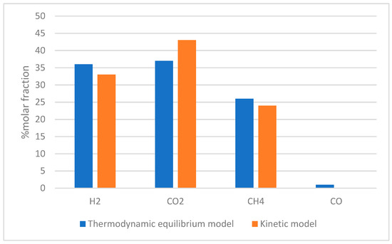
Figure 3.
Comparison of syngas composition at 600 °C [62].
Guan et al. [63] studied hydrothermal gasification of algae by means of a lumped first-order kinetic model, which was able to give the precise gas yield and also the effect of water density and biomass inlet on the final gas composition. Results from the kinetic model were compared with the results coming from a thermodynamic equilibrium model. Since results from both models were in good agreement, it is possible to conclude that kinetic models are able to predict equilibrium outcomes even if containing only methanation and water gas shift reactions. That means that only those two gas-phase reactions and their equilibrium constants can adequately describe the supercritical water gasification process in kinetic modeling.
Jin et al. [64] investigated the gasification of lignite by means of lumped method; at 560 °C, 25 MPa and residence time 4–12 s, they were able to predict the gas concentration (mainly composed of H2 and CO2, which were 6% and 34% respectively). The model prediction was in good agreement with experimental data obtained by means of a micro quartz tube reactor. Even if the lumped first-order method seems promising in estimating gas yield and gas composition, it is not flexible for all processes. For instance, it is not suitable to predict the syngas composition in supercritical water gasification, whose reaction conditions strongly depend on structures and distributions of pores in the feedstock material, which vary their structure along with the gasification process in turn affecting the reaction rate [65,66]. For this reason, some authors proposed a kinetic alternative model based on random pore size distribution. Vostrikov et al. [67] proposed a kinetic model based on random pore size distribution for the investigation of supercritical water gasification of coal. The study confirmed that the model is suitable for describing the rate of coal conversion dependent upon the coal conversion degree. Moreover, it was highlighted that random pore size distribution model is not trustable when catalytic effects occurred in non-uniform way. Sharma et al. [68] developed a 1-D kinetic model for biomass drying and pyrolysis. The results were validated against experimental test carried out at 350. 400 and 450 K, while the biomass flow rate, length and diameter of testing zone are 9 g/s, 50 cm and 25 cm respectively. The model showed a minor deviation from reality at lower temperature due the assumptions of the model, mainly for the effect of re-condensation of water vapor below re-condensation temperature.
Di Carlo et al. [69] developed a semi-empirical kinetic model for steam gasification via fluidized-bed gasifier. The reactor was a cylinder, and the model was based on a one-dimensional modeling of the mass and energy balance in order to calculate the syngas composition along the axis of the cylinder. The corresponding algorithm flowchart implemented by the authors is shown in Figure 4. Marcantonio et al. [52] compared the kinetic model developed by Di Carlo et al. with a thermodynamic equilibrium model and experimental data at 850 °C, S/B 0.25, and hazelnut shells as biomass feedstock. Results from the comparison are shown in Table 4. H2 and CH4 concentrations from both models are lower and higher, respectively, than the corresponding experimental data, and this is due to the presence of in-bed olivine in the real case that was neglected during modeling. Neglection of in-bed catalyst in modeling also determined a lower effect of water–gas shift reaction and steam–methane reforming reaction that caused an increase in CO concentration in modeling compared to the real case. The overprediction of CO caused the underprediction of CO2 due to the shifting of equilibrium of the water–gas shift reaction. It was noticed that even if the in-bed catalyst effect was included in the kinetic model, the final output did not change. Both models provided LHV, yield and cold gas efficiency in good agreement with experimental data.
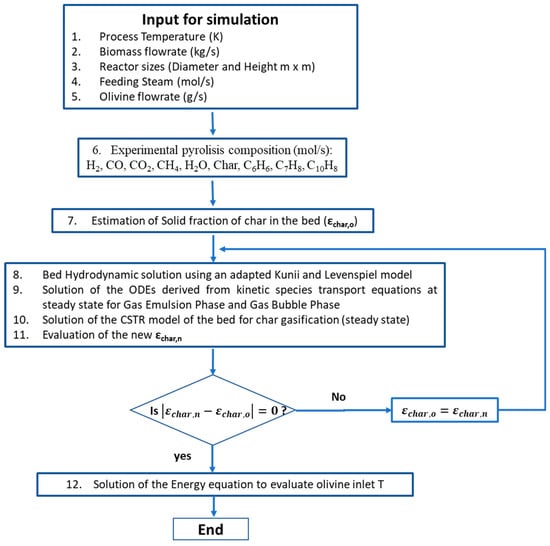
Figure 4.
Model algorithm flowchart developed by [69].
Table 4.
Comparison of syngas composition and characteristics (850 °C, S/B = 0.25) [52].
Kunii and Levenspiel [72] developed a hydrodynamic model in order to describe the multiphase (bubble and emulsion) nature of reacting mixture phases and their interaction.
The kin-semi approach helps simplify the complexity of kinetic models by assuming local equilibrium for specific reactions and/or gasifier zones, while concentrations and temperatures of the other reactions and/or zones are kinetically controlled [73,74,75]. The most common choice for the kin-semi model is to consider homogeneous gas-phase equilibria of reacting components from the step of pyrolysis: the equilibrium compositions are computed through three equilibrium constants or by minimizing Gibbs free energy.
Then, the produced gas mixture is mixed with the gasifying agent and char and becomes the inlet of a kinetic module where the final gas composition is computed using kinetic models [76,77]. The kin-semi approach is easier to use than the kin-total one: it needs less kinetic information and fewer parameters. For this reason, the kin-semi model provides more precise output results when the gas phase is near the chemical equilibrium.
To come to the point, kinetic models have the potential to indicate which reaction path is in charge of the production of a specific gaseous product and are also able to give precise output results only if the reaction rates, kinetic constant and gasifier geometry are well known. However, this means that these models are not flexible to use, since they must be developed precisely on a specific process with given conditions and since the required input information is not easy to obtain. On the other hand, it is possible to use simplified kinetic models providing quite accurate results for gas yield and gas composition. However, the simplified models are not able to identify which reaction produces a certain gas product, so when such information is needed, it is possible to overcome the limitations of the simplified models by coupling them with a CFD model.
5. CFD Models
CFD modeling is based on fluid mechanics principles and the use of numerical methods to solve Navier–Stokes equations [78,79]. It is a powerful tool to simulate the interaction among fluids that have surfaces inside specific boundary conditions. In the literature, there are several examples of CFD models to simulate biomass conversion processes such as thermochemical gasification [21,80,81] and pyrolysis [82,83]. CFD models are widely used to optimize the design of fluidized-bed reactors, since they are able to predict inert material concentration of in-bed gasifier, emissions, operational parameters, fuel-mixing efficiency, temperature profiles, heat flux, etc. [84,85].
It is possible to classify the CFD numerical approaches into three classes:
- ▪
- The Eulerian–Lagrangian discrete particle model (DPM), which considers gas a continuous and particle a discrete phase. It is used where there are diluted particle conditions, such as in the freeboard of the reactor. CFD DPMs consider particle trajectory in a continuous phase of fluid and take into account the interaction between particles by means of the heat and mass transfer as the governing phenomena [86,87]. The main advantage is the simple accounting of the particle size, allowing us to track the changes in physicochemical characteristics of the biomass particles during conversion along their path through the reactor.
- ▪
- The Eulerian–Eulerian two-fluid model (TFM), which is used to investigate both the gaseous and solid (particle) phase. Interaction of granular and continuous phases is considered via momentum transfer contribution based on drag models [88]. The CFD TFM approach has the disadvantages of high computational demand when a wide range of particle sizes has to be investigated because each size fraction of the distribution is counted as a separated phase. Moreover, another drawback of these models is that they are poor in recognizing the discrete character of the particle phase, so they are consequently poor in modeling flows of wide particles and in tracking movement and conversion of single particles.
- ▪
- The Eulerian–Eulerian discrete element model (DEM) within the Eulerian–Lagrangian framework, which uses the Eulerian method for the gas phase and discrete element method for the particle phase, tracking individually each particle and associating it with multiple physical (size, density, composition, and temperature) and thermochemical (reactive or inert) properties [89,90]. The main disadvantage of this method is the extremely small-time steps required, making this approach highly computationally demanding and thus best avoided for design and optimization of industrial scale facilities [91].
In the literature, many studies [92,93,94,95,96] investigated coal gasification in fluidized beds by means of the CDF TFM approach. Those studies showed great potential in modeling the gasification process, but at the same time, they still need to be improved in describing chemical reactions, especially the pyrolysis step.
Adnan et al. [97] made a comparison between the CDF TFM and CFD DPM, showing similar results for the fluid dynamics of a fluidized-bed gasifier. More in general, DPMs are more suitable for large-scale applications, where there is more independence from grids.
Ramos et al. [28] investigated results from a CFD TFM and CFD DEM, concluding that the latter gives a more accurate prediction. However, when the prediction is given for a local discrete temperature value, TFMs were demonstrated to be more accurate than DEMs. Moreover, the DEM approach requires about twice the time needed to execute the TFM.
In Figure 5, the validation of a CFD-DEM developed by Song et al. [89] against experimental data from [98] is shown. The comparison confirmed the applicability of such modeling for biomass gasification. It is possible to see that the developed model overpredicts CO and CO2 and underpredict H2 and CH4. This is likely due to the geometry and chemical reaction simplifications. Indeed, the model had a geometry simplification: 2-D was used instead of 3-D. This simplification affected the accuracy of results, since many researchers demonstrated that 2-D simulations are not able to reproduce the void fractions and velocity that can be achieved by a 3-D simulation [99]. Then, the chemical reaction path was defined through global reaction kinetics, rather than using all the heterogeneous and homogeneous reactions that coexist in the reactor, since most of those are still not totally understood and the corresponding kinetics are still unknown.

Figure 5.
Validation of a CFD-DEM [89] against experimental data from [98] at 820 °C and S/B = 0.8.
Tokmurzin et al. [100] developed a 3-D CFD model of biomass gasification in a fluidized-bed gasifier, taking into account the kinetic chemical model of the reactions involved in the process. The model was validated against the experimental data from [101] at 800 °C and air-to-fuel equivalent ratio in the range 0.2–0.3. The main deviation was found for CO2 (7% of deviation compared with experimental data), which was quite underpredicted by the simulation. This was likely due to the assumptions made while modeling that affected the concentration of oxygen available within the gasifier and also due to the use of simplified reaction rate expressions.
6. Process Modeling
Process modeling is a sequential approach in which each process is divided into unit operations and a series of equations are solved by means of kinetic or thermodynamic models. The most used software in this field is Aspen Plus [1,19,102]. Developed by Massachusetts Institute of Technology (MIT), Aspen Plus is a chemical engineering process optimization software that utilizes unit operation blocks, such as reactors, pumps, columns, heat exchangers, etc. Unit blocks are connected to each other through mass and energy streams, and this is represented in terms of a flowchart of the whole process. The software is based on a sub-sequential modular approach, and the simulation calculations use the in-built physical properties database [20]. The main advantage of Aspen Plus is that each unit can be analyzed independently and the properties of the outlet stream of each unit depend only on the inlet stream properties. In order to evaluate all physical properties of conventional components in the gaseous phase of the gasification process, the most suitable description is provided by the Peng–Robinson equation of state with the Boston–Mathias (PR-MB) modification [27], present in the default simulation setting of the Aspen Plus software. The evaluation of the enthalpy and density of the non-conventional components (biomass and ash) is obtained using the modules HCOALGEN and DCOALGEN, for enthalpy and density, respectively [27]. Those settings are meant for the general coal model, but they are now used for other non-conventional feedstock too, despite the reported deviations in the estimated heating value of biomass [103].
The main merits of process modeling are [12,25,31]:
- The whole process is taken into account (e.g., separators, mixers, heat exchangers, pumps, etc.) and not only the reaction unit.
- Overall energy duty of the process is estimated.
- Optimization to improve CAPEX and OPEX is allowed.
- The main assumptions for process modeling in Aspen Plus are:
- Process is steady-state and isothermal [104].
- Volatile products are H2, CO, CO2, CH4 and H2O [105].
- Char is 100% carbon [106].
- All gas mixtures are supposed to behave as perfect gases.
- Pressure drops and heat losses are neglected.
When process modeling is based on thermodynamic modeling, it is possible to obtain a QET approach also in process models, with the same benefits listed in Section 3—Thermodynamic models.
Several authors investigated biomass gasification process by means of Aspen Plus, demonstrating that it is a powerful tool to describe biomass gasification [12,107,108,109,110]. However, in the literature, there is a lack of scientific articles that point out the basic understanding of each model type and its applicability for designing a common biomass gasification process. In order to fill that gap, in Table 5 are shown the basic units that make up the gasification model, considering both the thermodynamic equilibrium and the kinetic approach.
Table 5.
Basic blocks for gasification process in Aspen Plus.
The three units listed in Table 5 are strictly required to develop a thermodynamic or kinetic process model by means of Aspen Plus software. Beyond the kinetic approach reported in Table 3, the semi-kinetic method using a DECOMP block (yield reactor) provides a simpler approach to convert the non-conventional inlet stream of biomass into its conventional components (carbon, hydrogen, oxygen, sulfur, nitrogen, and ash). The biomass ultimate analysis provides information to specify the yield distribution. Char gasification is performed in an CSTR introducing the reaction kinetics written through an external FORTRAN module [73] (see Figure 6). The separation column separates the volatile matter and solid matter, followed by a RGibbs reactor where the volatile combustion occurs, according to the hypothesis that reactions in the gaseous phase occur at Gibbs equilibrium. Moreover, the authors implemented hydrodynamic parameters to divide the gasifier in two parts, bed and freeboard, both modeled as CSTR reactors. Using FORTRAN code, each RCSTR is divided into a series of CSTR reactors of equal volume. The number of the elemental reactors depends on residence time, reactor dimensions, and operational conditions. Char gasification was performed in the RCSTR by means of kinetic reactions introduced through an external Fortran module. The model is used to predict the results of lab-scale gasification of pine with air and steam, and gave results in good agreement with experimental data.
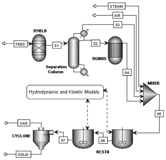
Figure 6.
A basic kinetic model for biomass gasification [73].
An example of the basic equilibrium process model, developed by Marcantonio et al. [27] by means of Aspen Plus software, is shown in Figure 7. The modeling was undertaken using the main units reported in Table 5 and adding a mixer to mix the biomass volatile stream with the gasifying agent stream (oxygen, steam, air, or a mix of them). Moreover, the total amount of char was split according to literature experimental data and only 89% went to the gasifier, while 11% was unreacted [110]. The simulative process was validated against experimental data, showing good correlation between simulations and experiments. The maximum error for the concentration of hydrogen, the main product of the gasification process, was 16.3%.
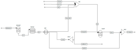
Figure 7.
A basic thermodynamic equilibrium model for biomass gasification [27].
As thermodynamic models, process models are not accurate at low temperatures or at large scales. To overcome such limitations, some authors suggested improving the equilibrium model with adjustable parameters and semi-empirical correlations [47].
7. Multivariate Data Analysis (MVDA) and Model Validation
In the ever-evolving fields of process and chemical engineering, managing and interpreting vast amounts of data are critical for optimizing processes, ensuring product quality, and making informed decisions [114,115]. In the area of biomass valorization and biorefinery processes, process control is particularly challenging due to the high variability of biomass (feed) properties [116,117]. For instance, Williams et al. [116] reviewed the effect of biomass property variability in different processes of energy conversion—fermentation, hydrothermal liquefaction, pyrolysis, and direct combustion—with a special focus on lignocellulosic feedstock. They underlined the relevance of some parameters, such as biomass moisture, in all process stages and on performance, even hindering the large-scale use of biomass as a carbon-neutral source for energy production.
Statistical methods can be used to manage the biomass variability [118]. Multivariate data analysis (MVDA) is a classical tool to extract meaningful insights from complex datasets, providing engineers with a deeper understanding of their systems and enabling them to enhance efficiency, reduce costs, and improve overall performance [115,119]. Multivariate data analysis (MVDA) focuses on uncovering the connections among variables by leveraging correlation patterns. In broader terms, MVDA enables the following [120]:
- Reducing the number of variables while maintaining the system’s descriptive capacity.
- Grouping variables into categories.
- Utilizing correlations between variables to characterize system behavior.
The simplest MVDA tool relies on the Pearson correlation coefficient, which establishes direct correlations between pairs of variables. However, in complex systems, this approach may not yield a definitive response, as a high correlation coefficient (close to unity in absolute value) does not always indicate a genuine causal relationship between the two variables. For instance, such a correlation might be the result of a third variable’s influence, which is independently highly correlated with both. Therefore, additional methods are necessary to elucidate the true interdependencies among variables.
Principal component analysis (PCA) [121] offers a solution by transforming the original variable dataset into a new set of orthogonal variables known as principal components (PC). Principal components (PCs) are linear combinations of the initial dataset. Let X = {[x]_1, [x]_2, ..., [x]_m} represent the original dataset with m variables (LCA outputs), recorded on n samples (statistical units). PCA transforms X into a new set of variables, PC = {P[C]_1, P[C]_2, ..., P[C]_k}, where k ≤ m. PCs are mutually orthogonal and ordered based on the descending values of explained variance. Given the PC set, the loading matrix L = {[λ]_((i,j))} reports the correlation coefficient between the i-th original variable, [x]_(i), and the j-th principal component P[C]_j, where each [λ]_((i,j)) represents a generic element in the matrix. Another tool of MVDA is canonical correlation analysis (CCA) [122]. CCA relies on initially dividing the entire dataset into two or more categories. Variables within each category are then combined linearly to generate k variables, known as canonical variables (CVs). The value of k corresponds to the minimum rank (number of variables) among all categories. The scores obtained through linear combinations aim to maximize the Pearson correlation coefficient between variables. As a result, CCA calculates the correlations between different classes (categories) of variables, effectively describing the system’s behavior. Consequently, a high correlation coefficient between the first canonical variables of two categories indicates a strong interdependency between the variables in those respective categories. Similarly, in the loading matrix L = {[λ]_((i,j))}, the generic element [λ]_((i,j)) denotes the correlation between the i-th canonical variable of a given category and the j-th variable from the original dataset. The complexity of the gasification reactions produces a large number of variables required to describe the kinetic and thermodynamic properties of the reacting phases. MVDA is an elective tool for the analysis of the resulting data set. Several works deal with the MVDA application to gasifiers, providing unique information for their optimization [111,123,124,125,126,127,128,129,130].
Gil et al. [131] adopted a multifaceted multivariate analysis of the data of gasification of 10 different biomasses (almond shells, chestnut sawdust, torrefied chestnut sawdust, cocoa shells, grape pomace, olive stones, pine leaves, pine sawdust, torrefied pine sawdust and pine kernel shells). The experimental data were collected in a bubbling fluidized-bed gasifier under an air–steam atmosphere. The analysis was carried out on the variables of the gasification outlet streams and biomass properties. The analysis included different MVDA methods, including PCA: the 10 different biomasses were classified into two groups according to their gasification products. The findings revealed that gasification of pine kernel shells, pine leaves, torrefied pine sawdust, olive stones, and pine sawdust resulted in substantial quantities of combustible gaseous products, including CO and CH. Additionally, their gasification exhibited high conversion rates and cold gas efficiency. Thus, it was inferred that C and H contents and the HHV of the biomass are the most important biomass properties for promoting the gas production, calorific value of the product gas, gasification conversion and energy efficiency. On the other hand, gasification of cocoa shells and grape pomace produced high H2 concentration and H2/CO molar ratio in the gas product, mainly due to the higher H/O ratio and K2O ash content of the biomass. Through a simple correlation analysis, the H2 concentration in the product gas was found to be negatively correlated with the O and volatile matter contents of the biomass.
All in all, this study demonstrated the potential of the MVDA in analyzing the gasification data, so as to reach valuable insight about the influence of the biomass properties on the gasification results.
Similarly, Dellavedova et al. [127] analyzed biomass characterization, gasification process conditions and obtained syngas properties from literature data by means of principal component analysis, showing again that biomass can be characterized and classified on the basis of its properties. This study showed that the most important variables for this model are the equivalence ratio (ER, i.e., the actual air fuel ratio divided by the stoichiometric air fuel ratio), the steam to biomass ratio (SB, i.e., the weight ratio between the amount of vapor used in the process and the biomass treated), the high heating value HHV, the carbon content, and temperature.
A strong direct correlation was observed between SB and the syngas characteristics. On the other hand, a negative correlation was found between syngas features and ER.
These two models show the potential of the MVDA in providing a data-driven description of gasification processes and, more in general, of complex reacting systems where the detailed description of all reactions and the characterization of the reactants can be very challenging.
Black-Box Approaches
Artificial neural network models are inspired by natural neurons: they are composed of a wide number of strictly interconnected processing elements, called neurons or nodes, working together at the same time to solve a given problem [132,133]. The nodes are organized in separated layers and interconnected with a given architecture. Each layer has a weight matrix, a bias vector, and an output vector [134].
This kind of model does not require physical description of the phenomena and is able to approximate arbitrary non-linear functions, which is why it was found to be a suitable approach to simulate and scale up complex biomass gasification process [30].
Puig-Arnavat et al. [30] proposed a model to predict gas composition and gas yield from biomass gasification in a fluidized-bed gasifier. The model structure developed by the authors is shown in Figure 8.

Figure 8.
ANN model structure to predict producer gas composition and gas yield from biomass gasification in a fluidized-bed gasifier [30].
Input and output variables used by Puig-Arnavat el al. [30] in their developed model are shown in Table 6.
Table 6.
Input and output variables in the ANN model of [30].
Results from the computational implementation of the ANN model were demonstrated to be in a good agreement with experiments.
Brown et al. [135] integrated an ANN approach with an equilibrium model for biomass gasification in a fluidized bed. The authors performed a non-linear regression with ANN to compute temperature changes, fuel composition and operational variables. They demonstrated that the application of the ANN model improved the accuracy of the equilibrium model and consequently the quantity of required input data decreased.
Sreejith et al. [136] developed an ANN model to predict the output gas composition, the heat content, and the temperature profile in a fluidized-bed gasifier. Results obtained from the model were in good agreement with experimental data: at steam to biomass of 2.5, the simulated result of H2 concentration was found to be 28.2%, while the experimental result was 29.1%.
Although the application of ANN method has yielded positive results in biomass gasification, there remains a scarcity of studies on the subject in the current literature. It is important to emphasize that ANN models are limited to the range of operating conditions used in their previous training. To enhance the effectiveness of ANN predictions, expanding the experimental database with a broader range of operating conditions could be highly beneficial.
8. Discussion
Table 7 shows features, pros, and cons of the three modeling approaches discussed in the previous paragraphs.
Table 7.
Description of gasification modeling approaches.
The choice of the model depends on the objectives and the experimental information available.
A first raw prediction of gasification process performance is well given by thermodynamic modeling, easy to implement and flexible to use, thanks to the independence of geometry. However, this approach does not give a realistic representation of the process at low temperature; moreover, it is not able to predict gasification process far from equilibrium (controlling kinetics and fluid dynamics phenomena, such as unconverted solid carbon and the formation of gaseous hydrocarbons).
Kinetic modeling gives a more accurate description of phenomena, but it requires a complete description of the reaction mechanisms, often unknown or only poorly known.
The main limitation of both kinetic and thermodynamic modeling in the investigation of gasification process is related to the interaction between solid- and gas-phase reactions, largely undescribed. In order to overcome this issue, CFD modeling is used to investigate interactions between solid- and gas-phase reactions involving a combined solution of mass, momentum, and energy balances, including turbulence regimes and multiphase hydrodynamics. In turn, the CFD computational complexity is very high, so it is reasonable to use if reliable experimental data are known and used as reference. The black-box approaches do not require any preliminary understanding or description of the physical phenomena.
Compared with other modeling approaches, ANN copes with non-linearity in a superior manner. Moreover, it does not require any mathematical or physical description of the phenomena and is able to adapt and learn. For those reasons, ANN modeling means the computational tool is able to update itself. On the other hand, it works only within the specific range of operational conditions it was trained on.
Finally, MVA and in general statistical methods provide insight about the correlation patterns of variables in the gasification process: this information is particularly valuable in cases of systems controlled by a large number of variables, such as in the case of gasification. High correlation may infer a causal link between variables, worth exploring through more detailed physical descriptions.
Additionally, correlation analysis is the basis for the sensitivity analysis, which guides the optimization methods for process engineering.
The number of published papers for each type of modeling for the last 10 years was investigated using Google Scholar. According to Figure 9, equilibrium models along with kinetic models and process models are the most studied. Papers about CFD models are still few, due to the complexity of the modeling, while ANN models are increasing. MVA analysis is still missing compared with the other models, but it is also slightly increasing (+14% from 2017 to 2020).
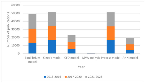
Figure 9.
Overview of gasification models over the past 10 years.
In summary, it is possible to affirm that black-box models with some empirical constraints are enough for preliminary predictions (e.g., quasi-equilibrium model).
Figure 10a–e briefly reports a schematic approach of each model.
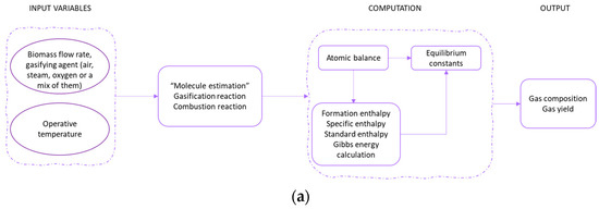

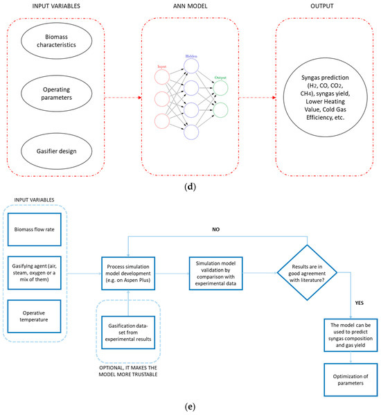
Figure 10.
Basic input/output diagram of (a) thermodynamic equilibrium modeling, (b) kinetic modeling, (c) CFD modeling, (d) ANN modeling, (e) process modeling for biomass gasification process.
9. An Overview on Tar Modeling Approach
To simplify modeling of gasification process, tar formation is typically not included [73,137,138]. However, an overview on the most relevant works is presented. Even if tar could form in hundreds of different chemical compounds, the modeling approach usually considers toluene, benzene and naphthalene as the main representative compounds [110,139,140]. Kinetic models involve reaction mechanisms comprising hundreds of elementary step-like reactions, which is why they are not favorable for tar modeling [141]. Zhao et al. [142] simulated toluene formation during the pyrolysis of biomass by simulation of thermodynamic equilibrium based on Gibbs free energy, showing a good agreement with literature experimental data. Serrano et al. [143] developed a tar model formation by means of an ANN approach, integrating different tar data coming from different experimental tests. The model predicted tar formation with good accuracy (R2 > 0.97).
In the last few years, some tar models were developed in Aspen Plus, due to the advances of the software [110,130,144]. A common way to simulate tar formation by means of the equilibrium approach is using a yield reactor setting the quantities of each tar compound according to the literature [145]. The most used proportions are 60%, 20% and 20% for benzene (C6H6), toluene (C7H8) and naphthalene (C10H8), respectively [144,146]. Puig-Garmero et al. [37] developed a process simulation of biomass gasification taking into account tar formation. The only tar considered was benzene, the formation of which was simulated into a Gibbs reactor, following the reaction:
They noted that increasing S/B ratio and/or temperature decreased tar formation. The deviation between the developed simulation and experimental results were imputed to be due to the neglection of kinetic factors in the model.
Palus et al. [147] integrated a tar formation model into an existing biomass gasification Aspen Plus model. Tar was modeled as CaHbOc and was converted into different components through a user-defined reactor. The authors noticed that the integration of tar modeling improves the prediction of hydrogen and carbon monoxide in the syngas. Tar formation is actually considered a challenge in gasification modeling, since it affects the syngas composition, resulting in a deviation between simulative composition and experimental results. Different hypotheses and modeling of tar formation make the process difficult, and it is not easy to conclude when it is better to include tar formation and when to neglect it.
10. Conclusions
A review of the most important and recent gasification modeling approaches was presented. Even if the most suitable choice of model is determined by factors including the scope of the simulation, the type of gasification reactor, the feedstock, and operational parameters, it is possible to make some general comments.
Equilibrium models are the simplest and easiest to develop and implement and have the benefit of being independent of reactor design. They are able to predict the maximum achievable yield of a desired product from a reacting system and the gas composition, but they lose their accuracy at low temperatures. Unlike equilibrium models, kinetic models predict the trend and the concentration of gas products at each position through the length of the reactor, also providing useful design assistance in estimating the possible limiting behavior of a system that is difficult or unsafe to reproduce experimentally. However, kinetic models are strictly dependent on geometry, and they cannot be used for systems different from the ones they are built for. CFD model results conform with experimental data in many cases. However, CFD models are computationally intensive and still have many approximations as well as assumptions, and there are several features of fluidized-bed reactors in which the application of CFD modeling still needs to be investigated (i.e., fuel combustion/gasification behavior during feeding, mixing of fuel in the dense bed, ash sintering, fuel characteristics, char reactivity, fragmentation of fuel in dense bed). In order to avoid complex processes and develop the simplest possible model that incorporates the principal gasification reactions and the gross physical characteristics of the reactor, process simulation models were developed using the process simulator Aspen Plus. Process simulation models are able to give a first raw evaluation of the overall energy duty and economics of the system, but they have all the pros and cons of the modeling they are based on (thermodynamic or kinetic modeling). ANN models offer some contribution to research in gasification process. The literature results show how the percentage composition of the four main gas species (H2, CO, CO2 and CH4) in producer gas and producer gas yield for a fluidized-bed gasifier can be successfully predicted by applying a neural network. However, ANN models still need to be trained and improved, and for this reason it is necessary to enlarge the literature database, adding more experimental data. MVA provides a good prediction of both dynamic behavior and equilibrium conditions, requiring a minimal computational burden, but it does not add any physical interpretation of the phenomena occurring.
Author Contributions
Conceptualization, M.C.; methodology, M.C. and L.D.P.; formal analysis, V.M.; investigation, V.M.; data curation, V.M., M.C. and L.D.P.; writing—original draft preparation, V.M. and L.D.P.; writing—review and editing, L.D.P., M.C. and M.D.F.; visualization, V.M.; supervision, M.C. All authors have read and agreed to the published version of the manuscript.
Funding
This research received no external funding.
Data Availability Statement
No new data were created.
Conflicts of Interest
The authors declare no conflict of interest.
Nomenclature
| Acronyms | ||
| ANN | artificial neural network | |
| CCA | canonical correlation analysis | |
| CFD | computational fluid dynamics | |
| CSTR | continuous-flow stirred-tank reactor | |
| DEM | discrete element method | |
| DPM | discrete particle model | |
| GMM | Gibbs free-energy gradient method model | |
| LHV | low heating value | |
| MVDA | multivariate data analysis | |
| QET | quasi-equilibrium temperature | |
| PCA | principal component analysis | |
| TFM | two-fluid model | |
| Symbols | Unit | Description |
| Cp,i | J/(mol·k) | specific heat at constant pressure of the i-component |
| H | kJ/mol | enthalpy |
| kJ/mol | enthalpy formation | |
| G | kJ/mol | Gibbs free energy |
| kJ/mol | Gibbs energy formation | |
| ni | mol | number of moles of the i-component |
| nT | mol | total moles of produced gas |
| P | Pa | pressure |
| Pi | Pa | partial pressure of i-component |
| P0 | Pa | operative pressure of the system |
| R | J/(mol·k) | universal constant of gas |
| T | K | temperature |
| Greek Letters | ||
| α | reaction coordinate of water–gas shift reaction | |
| β | reaction coordinate of steam-reforming reaction | |
| µi | chemical potential | |
| standard chemical potential of the i-component | ||
References
- Pala, L.P.R.; Wang, Q.; Kolb, G.; Hessel, V. Steam gasification of biomass with subsequent syngas adjustment using shift reaction for syngas production: An Aspen Plus model. Renew. Energy 2017, 101, 484–492. [Google Scholar] [CrossRef]
- Chang, W.-R.; Hwang, J.-J.; Wu, W. Environmental impact and sustainability study on biofuels for transportation applications. Renew. Sustain. Energy Rev. 2017, 67, 277–288. [Google Scholar] [CrossRef]
- Biagini, E.; Barontini, F.; Tognotti, L. Gasification of agricultural residues in a demonstrative plant: Vine pruning and rice husks. Bioresour. Technol. 2015, 194, 36–42. [Google Scholar] [CrossRef] [PubMed]
- Ritslaid, K.; Küüt, A.; Olt, J. State of the Art in Bioethanol Production. Agron. Res. 2010, 8, 236–254. [Google Scholar]
- Kuchler, M.; Linnér, B. Challenging the food vs. fuel dilemma: Genealogical analysis of the biofuel discourse pursued by international organizations. Food Policy 2012, 37, 581–588. [Google Scholar] [CrossRef]
- Antizar-Ladislao, B.; Turrion-Gomez, J.L. Second-generation biofuels and local bioenergy systems. Biofuels Bioprod. Biorefin. 2008, 2, 455–469. [Google Scholar] [CrossRef]
- Oliveira, W.E.; Franca, A.S.; Oliveira, L.S.; Rocha, S.D. Untreated coffee husks as biosorbents for the removal of heavy metals from aqueous solutions. J. Hazard. Mater. 2008, 152, 1073–1081. [Google Scholar] [CrossRef]
- Bolívar Caballero, J.J.; Zaini, I.N.; Yang, W. Reforming processes for syngas production: A mini-review on the current status, challenges, and prospects for biomass conversion to fuels. Appl. Energy Combust. Sci. 2022, 10, 100064. [Google Scholar] [CrossRef]
- Pande, M.; Bhaskarwar, A.N. Biomass conversion to energy. In Biomass Conversion; Springer: Berlin/Heidelberg, Germany, 2012; pp. 1–90. [Google Scholar] [CrossRef]
- Yilmaz, S.; Selim, H. A review on the methods for biomass to energy conversion systems design. Renew. Sustain. Energy Rev. 2013, 25, 420–430. [Google Scholar] [CrossRef]
- Ramzan, N.; Ashraf, A.; Naveed, S.; Malik, A. Simulation of hybrid biomass gasification using Aspen plus: A comparative performance analysis for food, municipal solid and poultry waste. Biomass Bioenergy 2011, 35, 3962–3969. [Google Scholar] [CrossRef]
- Liao, C.; Summers, M.; Seiser, R.; Cattolica, R.; Herz, R. Simulation of a pilot-scale dual-fluidized-bed gasifier for biomass. Environ. Prog. Sustain. Energy 2014, 33, 732–736. [Google Scholar] [CrossRef]
- Baldinelli, A.; Cinti, G.; Desideri, U.; Fantozzi, F. Biomass integrated gasifier-fuel cells: Experimental investigation on wood syngas tars impact on NiYSZ-anode Solid Oxide Fuel Cells. Energy Convers. Manag. 2016, 128, 361–370. [Google Scholar] [CrossRef]
- Arteaga-Pérez, L.E.; Casas-Ledón, Y.; Pérez-Bermúdez, R.; Peralta, L.M.; Dewulf, J.; Prins, W. Energy and exergy analysis of a sugar cane bagasse gasifier integrated to a solid oxide fuel cell based on a quasi-equilibrium approach. Chem. Eng. J. 2013. [CrossRef]
- Sikarwar, V.S.; Zhao, M.; Clough, P.; Yao, J.; Zhong, X.; Memon, M.Z.; Shah, N.; Anthony, J.; Fennell, P. An overview of advances in biomass gasification. Energy Envrion. Sci. 2016, 9, 2939–2977. [Google Scholar] [CrossRef]
- Parvez, A.M.; Hafner, S.; Hornberger, M.; Schmid, M.; Scheffknecht, G. Sorption enhanced gasification (SEG) of biomass for tailored syngas production with in-situ CO2 capture: Current status, process scale-up experiences and outlook. Renew. Sustain. Energy Rev. 2021, 141, 110756. [Google Scholar] [CrossRef]
- Dascomb, J.; Krothapalli, A.; Fakhrai, R. Thermal conversion efficiency of producing hydrogen enriched syngas from biomass steam gasification. Int. J. Hydrogen Energy 2013, 38, 11790–11798. [Google Scholar] [CrossRef]
- Hamel, S.; Krumm, W. Mathematical modelling and simulation of bubbling fluidised bed gasifiers. Powder Technol. 2001, 120, 105–112. [Google Scholar] [CrossRef]
- Ahmed, T.Y.; Ahmad, M.M.; Yusup, S.; Inayat, A.; Khan, Z. Mathematical and computational approaches for design of biomass gasification for hydrogen production: A review. Renew. Sustain. Energy Rev. 2012, 16, 2304–2315. [Google Scholar] [CrossRef]
- Patra, T.K.; Sheth, P.N. Biomass gasification models for downdraft gasifier: A state-of-the-art review. Renew. Sustain. Energy Rev. 2015, 50, 583–593. [Google Scholar] [CrossRef]
- Canneto, G.; Freda, C.; Braccio, G. Numerical simulation of gas-solid flow in an interconnected fluidized bed. Therm. Sci. 2015, 19, 317–328. [Google Scholar] [CrossRef]
- Ajorloo, M.; Ghodrat, M.; Scott, J.; Strezov, V. Recent advances in thermodynamic analysis of biomass gasification: A review on numerical modelling and simulation. J. Energy Inst. 2022, 102, 395–419. [Google Scholar] [CrossRef]
- Mazaheri, N.; Akbarzadeh, A.H.; Madadian, E.; Lefsrud, M. Systematic review of research guidelines for numerical simulation of biomass gasification for bioenergy production. Energy Convers. Manag. 2019, 183, 671–688. [Google Scholar] [CrossRef]
- Basu, P. Biomass Gasification and Pyrolysis: Practical Design and Theory; Academic Press: Cambridge, MA, USA, 2010. [Google Scholar]
- Ahmed, A.M.A.; Salmiaton, A.; Choong, T.S.Y.; Azlina, W.A.K.G.W. Review of kinetic and equilibrium concepts for biomass tar modeling by using Aspen Plus. Renew. Sustain. Energy Rev. 2015, 52, 1623–1644. [Google Scholar] [CrossRef]
- Baruah, D.; Baruah, D.C. Modeling of biomass gasification: A review. Renew. Sustain. Energy Rev. 2014, 39, 806–815. [Google Scholar] [CrossRef]
- Marcantonio, V.; Bocci, E.; Monarca, D. Development of a chemical quasi-equilibrium model of biomass waste gasification in a fluidized-bed reactor by using Aspen plus. Energies 2019, 13, 53. [Google Scholar] [CrossRef]
- Ramos, A.; Monteiro, E.; Rouboa, A. Numerical approaches and comprehensive models for gasification process: A review. Renew. Sustain. Energy Rev. 2019, 110, 188–206. [Google Scholar] [CrossRef]
- Li, Y.; Yan, L.; Yang, B.; Gao, W.; Farahani, M.R. Simulation of biomass gasification in a fluidized bed by artificial neural network (ANN). Energy Sources Part A Recov. Util. Environ. Eff. 2018, 40, 544–548. [Google Scholar] [CrossRef]
- Puig-Arnavat, M.; Hernández, J.A.; Bruno, J.C.; Coronas, A. Artificial neural network models for biomass gasification in fluidized bed gasifiers. Biomass Bioenergy 2013, 49, 279–289. [Google Scholar] [CrossRef]
- Safarian, S.; Unnþórsson, R.; Richter, C. A review of biomass gasification modelling. Renew. Sustain. Energy Rev. 2019, 110, 378–391. [Google Scholar] [CrossRef]
- Naaz, Z.; Ravi, M.R.; Kohli, S. Modelling and simulation of downdraft biomass gasifier: Issues and challenges. Biomass Bioenergy 2022, 162, 106483. [Google Scholar] [CrossRef]
- Nunes, L.J.R.; Rodrigues, A.M.; Matias, J.C.O.; Ferraz, A.I.; Rodrigues, A.C. Production of Biochar from Vine Pruning: Waste Recovery in the Wine Industry. Agriculture 2021, 11, 489. [Google Scholar] [CrossRef]
- Puig-Arnavat, M.; Bruno, J.C.; Coronas, A. Review and analysis of biomass gasification models. Renew. Sustain. Energy Rev. 2010, 14, 2841–2851. [Google Scholar] [CrossRef]
- Review of Technologies for Gasification of Biomass and Wastes. Final Report; E4tech. 2009. Available online: https://www.erm.com/service/low-carbon-economy-transition/ (accessed on 1 August 2023).
- Bridgwater, T. Biomass for energy. J. Sci. Food Agric. 2006, 86, 1755–1768. [Google Scholar] [CrossRef]
- Puig-Gamero, M.; Argudo-Santamaria, J.; Valverde, J.L.; Sánchez, P.; Sanchez-Silva, L. Three integrated process simulation using aspen plus®: Pine gasification, syngas cleaning and methanol synthesis. Energy Convers. Manag. 2018, 177, 416–427. [Google Scholar] [CrossRef]
- Eisavi, B.; Chitsaz, A.; Hosseinpour, J.; Ranjbar, F. Thermo-environmental and economic comparison of three different arrangements of solid oxide fuel cell-gas turbine (SOFC-GT) hybrid systems. Energy Convers. Manag. 2018, 168, 343–356. [Google Scholar] [CrossRef]
- Wang, J.; Diao, M.; Yue, K. Optimization on pinch point temperature difference of ORC system based on AHP-Entropy method. Energy 2016, 98, 790–797. [Google Scholar] [CrossRef]
- Wan, W.; Engvall, K.; Yang, W. Model investigation of condensation behaviors of alkalis during syngas treatment of pressurized biomass gasification. Chem. Eng. Process—Process Intensif. 2018, 129, 28–36. [Google Scholar] [CrossRef]
- Li, X.T.; Grace, J.R.; Lim, C.J.; Watkinson, A.P.; Chen, H.P.; Kim, J.R. Biomass gasification in a circulating fluidized bed. Biomass Bioenergy 2004, 26, 171–193. [Google Scholar] [CrossRef]
- Aydin, E.S.; Yucel, O.; Sadikoglu, H. Numerical and experimental investigation of hydrogen-rich syngas production via biomass gasification. Int. J. Hydrogen Energy 2018, 43, 1105–1115. [Google Scholar] [CrossRef]
- González-Vázquez, M.P.; Rubiera, F.; Pevida, C.; Pio, D.T.; Tarelho, L.A.C. Thermodynamic analysis of biomass gasification using aspen plus: Comparison of stoichiometric and non-stoichiometric models. Energies 2021, 14, 189. [Google Scholar] [CrossRef]
- Fiori, L.; Castello, D. Thermodynamic Analysis of the Supercritical Water Gasification of Biomass. In Near-Critical and Supercritical Water and Their Applications for Biorefineries. Biofuels and Biorefineries; Springer: Dordrecht, The Netherlands, 2014; pp. 99–129. [Google Scholar] [CrossRef]
- Barba, D.; Prisciandaro, M.; Salladini, A.; Mazziotti Di Celso, G. The Gibbs Free Energy Gradient Method for RDF gasification modelling. Fuel 2011, 90, 1402–1407. [Google Scholar] [CrossRef]
- Marcantonio, V.; De Falco, M.; Capocelli, M.; Bocci, E.; Colantoni, A.; Villarini, M. Process analysis of hydrogen production from biomass gasification in fluidized bed reactor with different separation systems. Int. J. Hydrogen Energy 2019, 44, 10350–10360. [Google Scholar] [CrossRef]
- Barba, D.; Capocelli, M.; Cornacchia, G.; Matera, D.A. Theoretical and experimental procedure for scaling-up RDF gasifiers: The Gibbs Gradient Method. Fuel 2016, 179, 60–70. [Google Scholar] [CrossRef]
- Gumz, W. Gas Producers and Blast Furnaces; Wiley: Hoboken, NJ, USA, 1950. [Google Scholar]
- Gambarotta, A.; Morini, M.; Zubani, A. A non-stoichiometric equilibrium model for the simulation of the biomass gasification process. Appl. Energy 2018, 227, 119–127. [Google Scholar] [CrossRef]
- Doherty, W.; Reynolds, A.; Kennedy, D.; Doherty, W.; Reynolds, A.; Kennedy, D. Simulation of a Circulating Fluidised Bed Biomass Gasifier using ASPEN Plus: A Performance Analysis. In Proceedings of the 21st International Conference on Efficiency, Cost, Optimization, Simulation and Environmental Impact of Energy Systems, Krakow, Poland, 24–27 June 2008; pp. 1241–1248. [Google Scholar]
- Mckeen, L.W.; Taylor, J.W. A study of the input data selection on the qet calculated intensities of ethylene and propane ions. Int. J. Mass Spectrom. Ion Phys. 1980, 33, 167–185. [Google Scholar] [CrossRef]
- Marcantonio, V.; Monforti Ferrario, A.; Di Carlo, A.; Del Zotto, L.; Monarca, D.; Bocci, E. Biomass Steam Gasification: A Comparison of Syngas Composition between a 1-D MATLAB Kinetic Model and a 0-D Aspen Plus Quasi-Equilibrium Model. Computation 2020, 8, 86. [Google Scholar] [CrossRef]
- Buekens, A.G.; Schoeters, J.G. Modelling of Biomass Gasification. In Fundamentals of Thermochemical Biomass Conversion; Overend, R.P., Milne, T.A., Mudge, L.K., Eds.; Springer: Dordrecht, The Netherlands, 1985; pp. 619–689. [Google Scholar]
- Loha, C.; Chatterjee, P.K.; Chattopadhyay, H. Performance of fluidized bed steam gasification of biomass—Modeling and experiment. Energy Convers. Manag. 2011, 52, 1583–1588. [Google Scholar] [CrossRef]
- Loha, C.; Chattopadhyay, H.; Chatterjee, P.K. Thermodynamic analysis of hydrogen rich synthetic gas generation from fluidized bed gasification of rice husk. Energy 2011, 36, 4063–4071. [Google Scholar] [CrossRef]
- Kaya, E.; Koksal, M. Investigation of the predicting ability of single-phase chemical equilibrium modeling applied to circulating fluidized bed coal gasification. J. Energy Resour. Technol. Trans. ASME 2016, 138, 032203. [Google Scholar] [CrossRef]
- Ramanan, M.V.; Lakshmanan, E.; Sethumadhavan, R.; Renganarayanan, S. Modeling and Experimental Validation of Cashew Nut Shell Char Gasification Adopting Chemical Equilibrium Approach. Energy Fuels 2008, 22, 2070–2078. [Google Scholar] [CrossRef]
- Bridgwater, A.V. The technical and economic feasibility of biomass gasification for power generation. Fuel 1995, 74, 631–653. [Google Scholar] [CrossRef]
- Basu, P.; Kaushal, P. Modeling of pyrolysis and gasification of biomass in fluidized beds: A review. Chem. Prod. Process Model. 2009, 4. [Google Scholar] [CrossRef]
- Castello, D.; Fiori, L. Kinetics modeling and main reaction schemes for the supercritical water gasification of methanol. J. Supercrit. Fluids 2012, 69, 64–74. [Google Scholar] [CrossRef]
- Ranzi, E.; Dente, M.; Goldaniga, A.; Bozzano, G.; Faravelli, T. Lumping procedures in detailed kinetic modeling of gasification, pyrolysis, partial oxidation and combustion of hydrocarbon mixtures. Prog. Energy Combust. Sci. 2001, 27, 99–139. [Google Scholar] [CrossRef]
- Resende, F.L.P.; Savage, P.E. Kinetic model for noncatalytic supercritical water gasification of cellulose and lignin. AIChE J. 2010, 56, 2412–2420. [Google Scholar] [CrossRef]
- Guan, Q.; Wei, C.; Savage, P.E. Kinetic model for supercritical water gasification of algae. Phys. Chem. Chem. Phys. 2012, 14, 3140–3147. [Google Scholar] [CrossRef] [PubMed]
- Jin, H.; Guo, L.; Guo, J.; Ge, Z.; Cao, C.; Lu, Y. Study on gasification kinetics of hydrogen production from lignite in supercritical water. Int. J. Hydrogen Energy 2015, 40, 7523–7529. [Google Scholar] [CrossRef]
- Iwaszenko, S.; Howaniec, N.; Smoliński, A. Determination of random pore model parameters for underground coal gasification simulation. Energy 2019, 166, 972–978. [Google Scholar] [CrossRef]
- Experimental Investigation on the Gasification Kinetic Model of a Char Particle in Supercritical Water n.d. Available online: https://agris.fao.org/agris-search/search.do?recordID=US201700052980 (accessed on 19 May 2023).
- Vostrikov, A.A.; Psarov, S.A.; Dubov, D.Y.; Fedyaeva, O.N.; Sokol, M.Y. Kinetics of coal conversion in supercritical water. Energy Fuels 2007, 21, 2840–2845. [Google Scholar] [CrossRef]
- Sharma, A.K. Modeling Drying and Pyrolysis of Moist Wood Particles at Slow Heating Rates. Int. J. Energy Environ. Eng. 2019, 13, 243–250. [Google Scholar] [CrossRef]
- Di Carlo, A.; Borello, D.; Bocci, E. Process simulation of a hybrid SOFC/mGT and enriched air/steam fluidized bed gasifier power plant. Int. J. Hydrogen Energy 2013, 38, 5857–5874. [Google Scholar] [CrossRef]
- Fercher, E.; Hofbauer, H.; Fleck, T.; Rauch, R.; Veronik, G. Two years experience with the ficfb-gasification process. In Proceedings of the 10th European Conference and Technology Exhibition Biomass for Energy and Industry, Würzburg, Germany, 8–11 June 1998. [Google Scholar]
- Pfeifer, C.; Rauch, R.; Hofbauer, H. In-Bed Catalytic Tar Reduction in a Dual Fluidized Bed Biomass Steam Gasifier. Ind. Eng. Chem. Res. 2004, 43, 1634–1640. [Google Scholar] [CrossRef]
- Kunii, D.; Levenspiel, O. Fluidized reactor models. 1. For bubbling beds of fine, intermediate, and large particles. 2. For the lean phase: Freeboard and fast fluidization. Ind. Eng. Chem. Res. 1990, 29, 1226–1234. [Google Scholar] [CrossRef]
- Nikoo, M.B.; Mahinpey, N. Simulation of biomass gasification in fluidized bed reactor using ASPEN PLUS. Biomass Bioenergy 2008, 32, 1245–1254. [Google Scholar] [CrossRef]
- Roy, P.C.; Datta, A.; Chakraborty, N. Assessment of cow dung as a supplementary fuel in a downdraft biomass gasifier. Renew. Energy 2010, 35, 379–386. [Google Scholar] [CrossRef]
- Roy, P.C.; Datta, A.; Chakraborty, N. An assessment of different biomass feedstocks in a downdraft gasifier for engine application. Fuel 2013, 106, 864–868. [Google Scholar] [CrossRef]
- Jia, J.; Xu, L.; Abudula, A.; Sun, B. Effects of operating parameters on performance of a downdraft gasifier in steady and transient state. Energy Convers. Manag. 2018, 155, 138–146. [Google Scholar] [CrossRef]
- Kaushal, P.; Tyagi, R. Advanced simulation of biomass gasification in a fluidized bed reactor using ASPEN PLUS. Renew. Energy 2017, 101, 629–636. [Google Scholar] [CrossRef]
- Lu, Y.; Huang, J.; Zheng, P. Fluid hydrodynamic characteristics in supercritical water fluidized bed: A DEM simulation study. Chem. Eng. Sci. 2014, 117, 283–292. [Google Scholar] [CrossRef]
- Gómez-Barea, A.; Leckner, B. Modeling of biomass gasification in fluidized bed. Prog. Energy Combust. Sci. 2010, 36, 444–509. [Google Scholar] [CrossRef]
- Xue, Q.; Fox, R.O. Reprint of: Multi-fluid CFD modeling of biomass gasification in polydisperse fluidized-bed gasifiers. Powder Technol. 2014, 265, 23–34. [Google Scholar] [CrossRef]
- Hassen, W.; Dhrioua, M.; Kolsi, L.; Anbumalar, V.; Al-Rashed, A.A.A.A.; Borjini, M.N. CFD modeling of gas-particles flow in a circulating fluidized G-Volution gasification reactor. Int. J. Mech. Sci. 2018, 144, 438–451. [Google Scholar] [CrossRef]
- Papadikis, K.; Gu, S.; Bridgwater, A.V.; Gerhauser, H. Application of CFD to model fast pyrolysis of biomass. Fuel Process Technol. 2009, 90, 504–512. [Google Scholar] [CrossRef]
- Xue, Q.; Dalluge, D.; Heindel, T.J.; Fox, R.O.; Brown, R.C. Experimental validation and CFD modeling study of biomass fast pyrolysis in fluidized-bed reactors. Fuel 2012, 97, 757–769. [Google Scholar] [CrossRef]
- Nguyen, T.D.B.; Seo, M.W.; Lim YIl Song, B.H.; Kim, S.D. CFD simulation with experiments in a dual circulating fluidized bed gasifier. Comput. Chem. Eng. 2012, 36, 48–56. [Google Scholar] [CrossRef]
- Herce, C.; Cortés, C.; Stendardo, S. Numerical simulation of a bubbling fluidized bed reactor for sorption-enhanced steam methane reforming under industrially relevant conditions: Effect of sorbent (dolomite and CaO-Ca 12 Al 14 O 33 ) and operational parameters. Fuel Process Technol. 2019, 186, 137–148. [Google Scholar] [CrossRef]
- Barik, H.; Bhattacharya, S.; Bose, M. CFD-DPM-based numerical simulation for char gasification in an entrained flow reactor: Effect of residence time distribution. Can. J. Chem. Eng. 2023, 101, 2286–2306. [Google Scholar] [CrossRef]
- Salem, A.M.; Paul, M.C. CFD modelling of spatiotemporal evolution of detailed tar species in a downdraft gasifier. Biomass Bioenergy 2023, 168, 106656. [Google Scholar] [CrossRef]
- von Berg, L.; Anca-Couce, A.; Hochenauer, C.; Scharler, R. Multi-scale modelling of fluidized bed biomass gasification using a 1D particle model coupled to CFD. Fuel 2022, 324, 124677. [Google Scholar] [CrossRef]
- Wang, S.; Luo, K.; Fan, J. CFD-DEM coupled with thermochemical sub-models for biomass gasification: Validation and sensitivity analysis. Chem. Eng. Sci. 2020, 217, 115550. [Google Scholar] [CrossRef]
- Ku, X.; Li, T.; Løvås, T. CFD–DEM simulation of biomass gasification with steam in a fluidized bed reactor. Chem. Eng. Sci. 2015, 122, 270–283. [Google Scholar] [CrossRef]
- Lungu, M.; Siame, J.; Mukosha, L. Comparison of CFD-DEM and TFM approaches for the simulation of the small scale challenge problem 1. Powder Technol. 2021, 378, 85–103. [Google Scholar] [CrossRef]
- Yu, L.; Lu, J.; Zhang, X.; Zhang, S. Numerical simulation of the bubbling fluidized bed coal gasification by the kinetic theory of granular flow (KTGF). Fuel 2007, 86, 722–734. [Google Scholar] [CrossRef]
- Armstrong, L.M.; Gu, S.; Luo, K.H. Parametric Study of Gasification Processes in a BFB Coal Gasifier. Ind. Eng. Chem. Res. 2011, 50, 5959–5974. [Google Scholar] [CrossRef]
- Armstrong, L.M.; Gu, S.; Luo, K.H. Effects of limestone calcination on the gasification processes in a BFB coal gasifier. Chem. Eng. J. 2011, 168, 848–860. [Google Scholar] [CrossRef]
- Yang, S.; Liu, X.; Wang, S. CFD simulation of air-blown coal gasification in a fluidized bed reactor with continuous feedstock. Energy Convers. Manag. 2020, 213, 112774. [Google Scholar] [CrossRef]
- Xia, Z.; Fan, Y.; Wang, T.; Guo, X.; Chen, C. A TFM-KTGF jetting fluidized bed coal gasification model and its validations with data of a bench-scale gasifier. Chem. Eng. Sci. 2015, 131, 12–21. [Google Scholar] [CrossRef]
- Adnan, M.; Sun, J.; Ahmad, N.; Wei, J.J. Comparative CFD modeling of a bubbling bed using a Eulerian–Eulerian two-fluid model (TFM) and a Eulerian-Lagrangian dense discrete phase model (DDPM). Powder Technol. 2021, 383, 418–442. [Google Scholar] [CrossRef]
- Song, T.; Wu, J.; Shen, L.; Xiao, J. Experimental investigation on hydrogen production from biomass gasification in interconnected fluidized beds. Biomass Bioenergy 2012, 36, 258–267. [Google Scholar] [CrossRef]
- Li, T.; Pannala, S.; Shahnam, M. Reprint of "CFD simulations of circulating fluidized bed risers, part II, evaluation of differences between 2D and 3D simulations. Powder Technol. 2014, 265, 13–22. [Google Scholar] [CrossRef]
- Tokmurzin, D.; Nam, J.Y.; Park, S.J.; Yoon, S.J.; Mun, T.Y.; Yoon, S.M.; Moon, J.H.; Lee, J.G.; Lee, D.H.; Ra, H.W.; et al. Three-Dimensional CFD simulation of waste plastic (SRF) gasification in a bubbling fluidized bed with detailed kinetic chemical model. Energy Convers. Manag. 2022, 267, 115925. [Google Scholar] [CrossRef]
- Han, S.W.; Lee, J.J.; Tokmurzin, D.; Lee, S.H.; Nam, J.Y.; Park, S.J.; Ra, H.W.; Mun, T.Y.; Yoon, S.J.; Yoon, S.M.; et al. Gasification characteristics of waste plastics (SRF) in a bubbling fluidized bed: Effects of temperature and equivalence ratio. Energy 2022, 238, 121944. [Google Scholar] [CrossRef]
- Doherty, W.; Reynolds, A.; Kennedy, D. Aspen Plus Simulation of Biomass Gasification in a Steam Blown Dual Fluidised Bed. In Materials and Processes for Energy: Communicating Current Research and Technological Developments; Formatex Research Centre: Badajoz, Spain, 2013. [Google Scholar]
- Mutlu, Ö.Ç.; Zeng, T. Challenges and Opportunities of Modeling Biomass Gasification in Aspen Plus: A Review. Chem. Eng. Technol. 2020, 43, 1674–1689. [Google Scholar] [CrossRef]
- Ye, G.; Xie, D.; Qiao, W.; Grace, J.R.; Lim, C.J. Modeling of fluidized bed membrane reactors for hydrogen production from steam methane reforming with Aspen Plus. Int. J. Hydrogen Energy 2009, 34, 4755–4762. [Google Scholar] [CrossRef]
- Sadaka, S.S.; Ghaly, A.E.; Sabbah, M.A. Two phase biomass air-steam gasification model for fluidized bed reactors: Part I—Model development. Biomass Bioenergy 2002, 22, 439–462. [Google Scholar] [CrossRef]
- Demirbaş, A. Carbonization ranking of selected biomass for charcoal, liquid and gaseous products. Energy Convers. Manag. 2001, 42, 1229–1238. [Google Scholar] [CrossRef]
- Doherty, W.; Reynolds, A.; Kennedy, D. Computer simulation of a biomass gasification-solid oxide fuel cell power system using Aspen Plus. Energy 2010, 27, 415–427. [Google Scholar] [CrossRef]
- Batista, F.R.M.; Follegatti-Romero, L.A.; Bessa, L.C.B.A.; Meirelles, A.J.A. Computational simulation applied to the investigation of industrial plants for bioethanol distillation. Comput. Chem. Eng. 2012, 46, 1–16. [Google Scholar] [CrossRef]
- Detchusananard, T.; Ponpesh, P.; Saebea, D.; Authayanun, S.; Arpornwichanop, A. Modeling and analysis of sorption enhanced chemical looping biomass gasification. Chem. Eng. Trans. 2017, 57, 103–108. [Google Scholar] [CrossRef]
- Marcantonio, V.; De Falco, M.; Capocelli, M.; Amado-Fierro, Á.; Centeno, T.A.; Bocci, E. Modelling and assessment of a sorption enhanced gasification system coupled with hydrothermal carbonization, hot gas cleaning, and plasma to produce pure H2 from biomass. Int. J. Hydrogen Energy 2023, 48, 32672–32685. [Google Scholar] [CrossRef]
- Dang, Q.; Zhang, X.; Zhou, Y.; Jia, X. Prediction and optimization of syngas production from a kinetic-based biomass gasification process model. Fuel Process Technol. 2021, 212, 106604. [Google Scholar] [CrossRef]
- Peters, J.F.; Banks, S.W.; Bridgwater, A.V.; Dufour, J. A kinetic reaction model for biomass pyrolysis processes in Aspen Plus. Appl. Energy 2017, 188, 595–603. [Google Scholar] [CrossRef]
- Di Blasi, C. Modeling chemical and physical processes of wood and biomass pyrolysis. Prog. Energy Combust. Sci. 2008, 34, 47–90. [Google Scholar] [CrossRef]
- Krijnen, W.P.; Wit, E. Computational and Statistical Methods for Chemical Engineering; Chapman and Hall/CRC: New York, NY, USA, 2022. [Google Scholar]
- Ge, Z.; Song, Z. Process Monitoring Based on Independent Component Analysis−Principal Component Analysis (ICA−PCA) and Similarity Factors. Ind. Eng. Chem. Res. 2007, 46, 2054–2063. [Google Scholar] [CrossRef]
- Williams, C.L.; Westover, T.L.; Emerson, R.M.; Tumuluru, J.S.; Li, C. Sources of Biomass Feedstock Variability and the Potential Impact on Biofuels Production. Bioenergy Res. 2016, 9, 1–14. [Google Scholar] [CrossRef]
- Resch, M.G.; Ladisch, M.R. Analysis, Impacts, and Solutions to Biomass Variability for Production of Fuels and Value-Added Products. ACS Sustain. Chem. Eng. 2020, 8, 15375–15377. [Google Scholar] [CrossRef]
- Martínez, M.G.; Floquet, P.; Dupont, C.; da Silva Perez, D.; Meyer, X.M. Assessing the impact of woody and agricultural biomass variability on its behaviour in torrefaction through Principal Component Analysis. Biomass Bioenergy 2020, 134, 105474. [Google Scholar] [CrossRef]
- Multivariate Statistical Process Control and Industrial Applications—ProQuest n.d. Available online: https://www.proquest.com/openview/207b6bafd5110b23915b2f4994723514/1?pq-origsite=gscholar&cbl=39817 (accessed on 31 July 2023).
- Clark, V. Multivariate data analysis in industrial practice: By Paul J. LEWI John Wiley and Sons, Chichester, 1982 (256 pp., $29.95/£13.75, ISBN 0471 10466 3). Comput. Stat. Data Anal. 1983, 1, 289–290. [Google Scholar] [CrossRef]
- Jolliffe, I.T. Principal Component Analysis for Special Types of Data. In Principal Component Analysis; Springer: New York, NY, USA, 2002; pp. 338–372. [Google Scholar] [CrossRef]
- Thompson, B. Canonical Correlation Analysis: Uses and Interpretation. Available online: https://books.google.com.hk/books?hl=en&lr=&id=Dk0XINOvsw8C&oi=fnd&pg=PA11&dq=Canonical+Correlation+Analysis:+Uses+and+Interpretation&ots=3bDBW84Vpj&sig=kIJ6zi3v3HqI-8sDHWjFINPB7ks&redir_esc=y#v=onepage&q=Canonical%20Correlation%20Analysis%3A%20Uses%20and%20Interpretation&f=false (accessed on 31 July 2023).
- Nachtergaele, P.; Thybaut, J.; De Meester, S.; Drijvers, D.; Saeys, W.; Dewulf, J. Multivariate Analysis of Industrial Biorefinery Processes: Strategy for Improved Process Understanding with Case Studies in Fatty Acid Production. Ind. Eng. Chem. Res. 2020, 59, 7732–7745. [Google Scholar] [CrossRef]
- Li, J.; Xu, K.; Yao, X.; Chen, S. Prediction and optimization of syngas production from steam gasification: Numerical study of operating conditions and biomass composition. Energy Convers. Manag. 2021, 236, 114077. [Google Scholar] [CrossRef]
- Meuzelaar, H.L.C.; Hoesterey, B.L.; Windig, W.; Hill, G.R. Prediction and modeling of coal conversion reactions by pyrolysis mass spectrometry and multivariate statistical analysis. Fuel Process Technol. 1987, 15, 59–70. [Google Scholar] [CrossRef]
- Tiong, L.; Komiyama, M. Statistical analysis of microalgae supercritical water gasification: Reaction variables, catalysis and reaction pathways. J. Supercrit. Fluids 2022, 183, 105552. [Google Scholar] [CrossRef]
- Dellavedova, M.; Derudi, M.; Biesuz, R.; Lunghi, A.; Rota, R. On the gasification of biomass: Data analysis and regressions. Process Saf. Environ. Prot. 2012, 90, 246–254. [Google Scholar] [CrossRef]
- Motta, I.L.; Marchesan, A.N.; Maciel Filho, R.; Wolf Maciel, M.R. Correlating biomass properties, gasification performance, and syngas applications of Brazilian feedstocks via simulation and multivariate analysis. Ind. Crops Prod. 2022, 181, 114808. [Google Scholar] [CrossRef]
- Baggio, P.; Baratieri, M.; Fiori, L.; Grigiante, M.; Avi, D.; Tosi, P. Experimental and modeling analysis of a batch gasification/pyrolysis reactor. Energy Convers. Manag. 2009, 50, 1426–1435. [Google Scholar] [CrossRef]
- Adeyemi, I.; Janajreh, I.; Arink, T.; Ghenai, C. Gasification behavior of coal and woody biomass: Validation and parametrical study. Appl. Energy 2017, 185, 1007–1018. [Google Scholar] [CrossRef]
- Gil, M.V.; González-Vázquez, M.P.; García, R.; Rubiera, F.; Pevida, C. Assessing the influence of biomass properties on the gasification process using multivariate data analysis. Energy Convers. Manag. 2019, 184, 649–660. [Google Scholar] [CrossRef]
- Obafemi, O.; Stephen, A.; Ajayi, O.; Nkosinathi, M. A survey of Artificial Neural Network-based Prediction Models for Thermal Properties of Biomass. Procedia Manuf. 2019, 33, 184–191. [Google Scholar] [CrossRef]
- George, J.; Arun, P.; Muraleedharan, C. Assessment of producer gas composition in air gasification of biomass using artificial neural network model. Int. J. Hydrogen Energy 2018, 43, 9558–9568. [Google Scholar] [CrossRef]
- Ranade, N.V.; Nagarajan, S.; Sarvothaman, V.; Ranade, V.V. ANN based modelling of hydrodynamic cavitation processes: Biomass pre-treatment and wastewater treatment. Ultrason. Sonochem. 2021, 72, 105428. [Google Scholar] [CrossRef]
- Brown, D.; Fuchino, T.; Maréchal, F. Solid fuel decomposition modelling for the design of biomass gasification systems. Comput. Aided Chem. Eng. 2006, 21, 1661–1666. [Google Scholar] [CrossRef]
- Sreejith, C.C.; Muraleedharan, C.; Arun, P. Performance prediction of fluidised bed gasification of biomass using experimental data-based simulation models. Biomass Convers. Biorefinery 2013, 3, 283–304. [Google Scholar] [CrossRef]
- Begum, S.; Rasul, M.G.; Akbar, D.; Ramzan, N. Performance analysis of an integrated fixed bed gasifier model for different biomass feedstocks. Energies 2013, 6, 6508–6524. [Google Scholar] [CrossRef]
- Hussain, M.; Tufa, L.D.; Yusup, S.; Zabiri, H. A kinetic-based simulation model of palm kernel shell steam gasification in a circulating fluidized bed using Aspen Plus®: A case study. Biofuels 2018, 9, 635–646. [Google Scholar] [CrossRef]
- Furusawa, T.; Saito, K.; Kori, Y.; Miura, Y.; Sato, M.; Suzuki, N. Steam reforming of naphthalene/benzene with various types of Pt- and Ni-based catalysts for hydrogen production. Fuel 2013, 103, 111–121. [Google Scholar] [CrossRef]
- Herrmann, T.; Dillig, M.; Hauth, M.; Karl, J. Conversion of tars on solid oxide fuel cell anodes and its impact on voltages and current densities. Energy Sci. Eng. 2017, 5, 194–207. [Google Scholar] [CrossRef]
- Font Palma, C. Modelling of tar formation and evolution for biomass gasification: A review. Appl. Energy 2013, 111, 129–141. [Google Scholar] [CrossRef]
- Zhao, B.; Zhang, X.; Chen, L.; Qu, R.; Meng, G.; Yi, X.; Sun, L. Steam reforming of toluene as model compound of biomass pyrolysis tar for hydrogen. Biomass Bioenergy 2010, 34, 140–144. [Google Scholar] [CrossRef]
- Serrano, D.; Castelló, D. Tar prediction in bubbling fluidized bed gasification through artificial neural networks. Chem. Eng. J. 2020, 402, 126229. [Google Scholar] [CrossRef]
- Damartzis, T.; Michailos, S.; Zabaniotou, A. Energetic assessment of a combined heat and power integrated biomass gasification–internal combustion engine system by using Aspen Plus®. Fuel Process Technol. 2012, 95, 37–44. [Google Scholar] [CrossRef]
- Rapagnà, S.; Orazio, A.D.; Gallucci, K.; Ugo, P. Hydrogen Rich Gas from Catalytic Steam Gasification of Biomass in a Fluidized Bed Containing Catalytic Filters. Chem. Eng. Trans. 2014, 37, 157–162. [Google Scholar]
- Marcantonio, V.; Bocci, E.; Ouweltjes, J.P.; Del Zotto, L.; Monarca, D. Evaluation of sorbents for high temperature removal of tars, hydrogen sulphide, hydrogen chloride and ammonia from biomass-derived syngas by using Aspen Plus. Int. J. Hydrogen Energy 2020, 45, 6651–6662. [Google Scholar] [CrossRef]
- Pauls, J.H.; Mahinpey, N.; Mostafavi, E. Simulation of air-steam gasification of woody biomass in a bubbling fluidized bed using Aspen Plus: A comprehensive model including pyrolysis, hydrodynamics and tar production. Biomass Bioenergy 2016, 95, 157–166. [Google Scholar] [CrossRef]
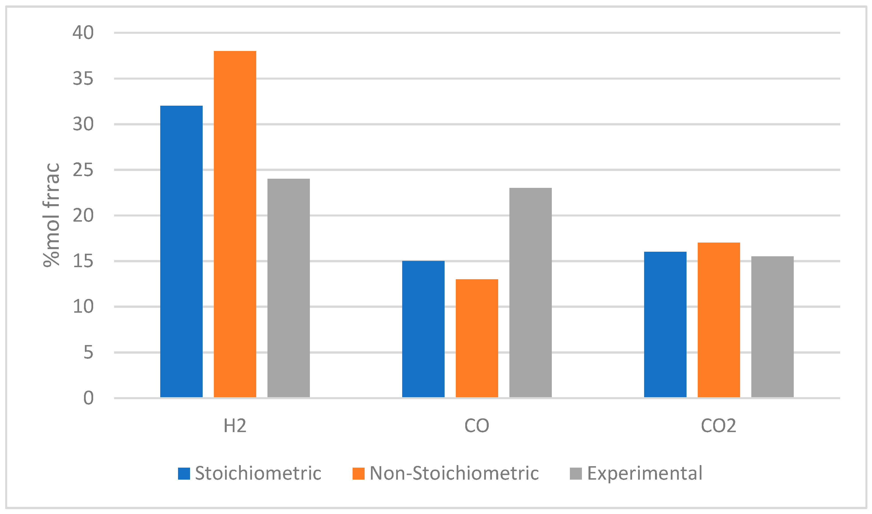
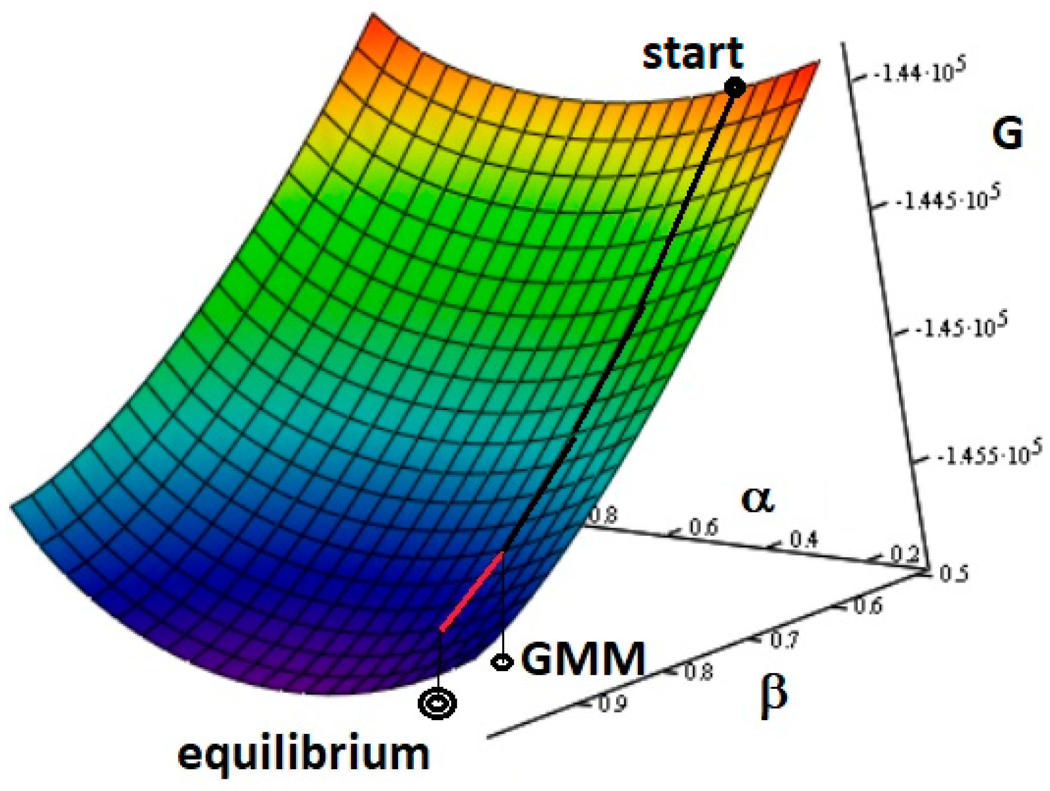
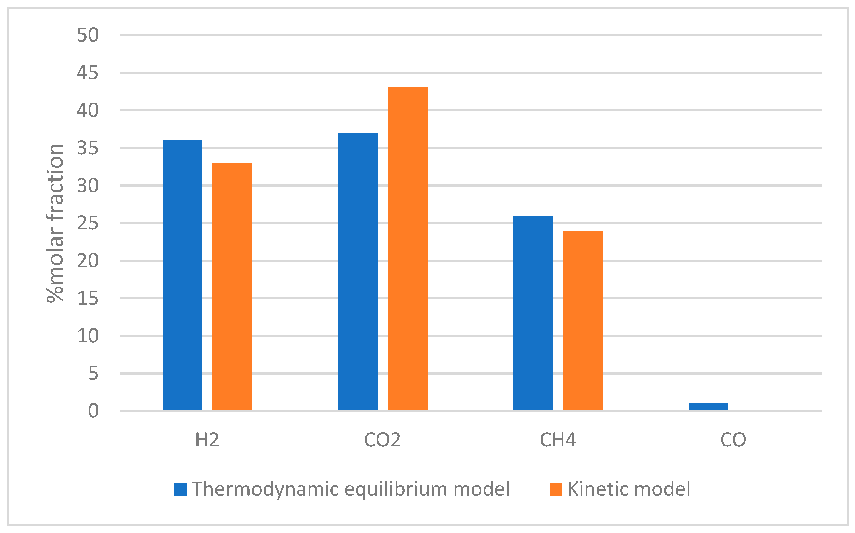
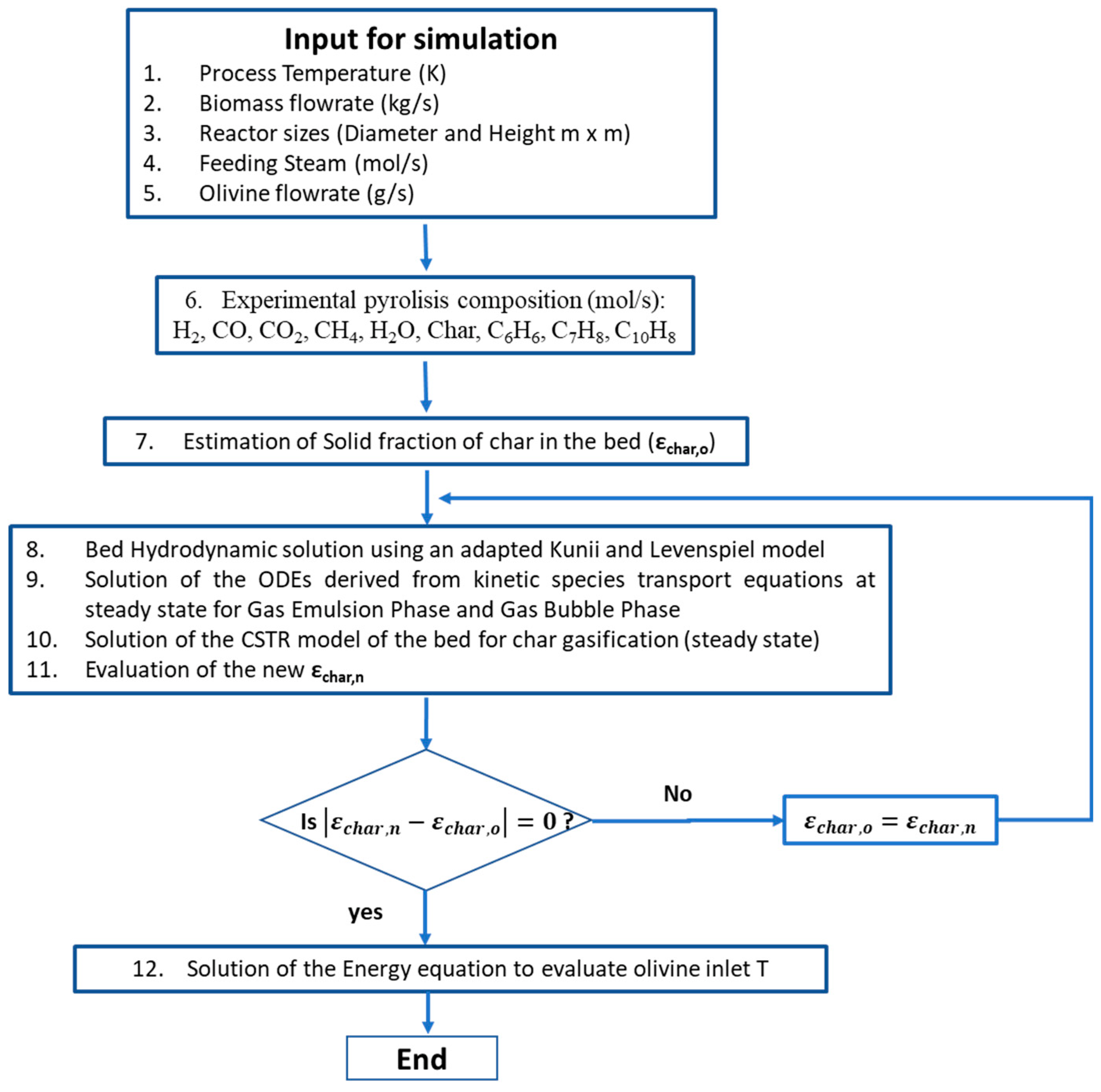
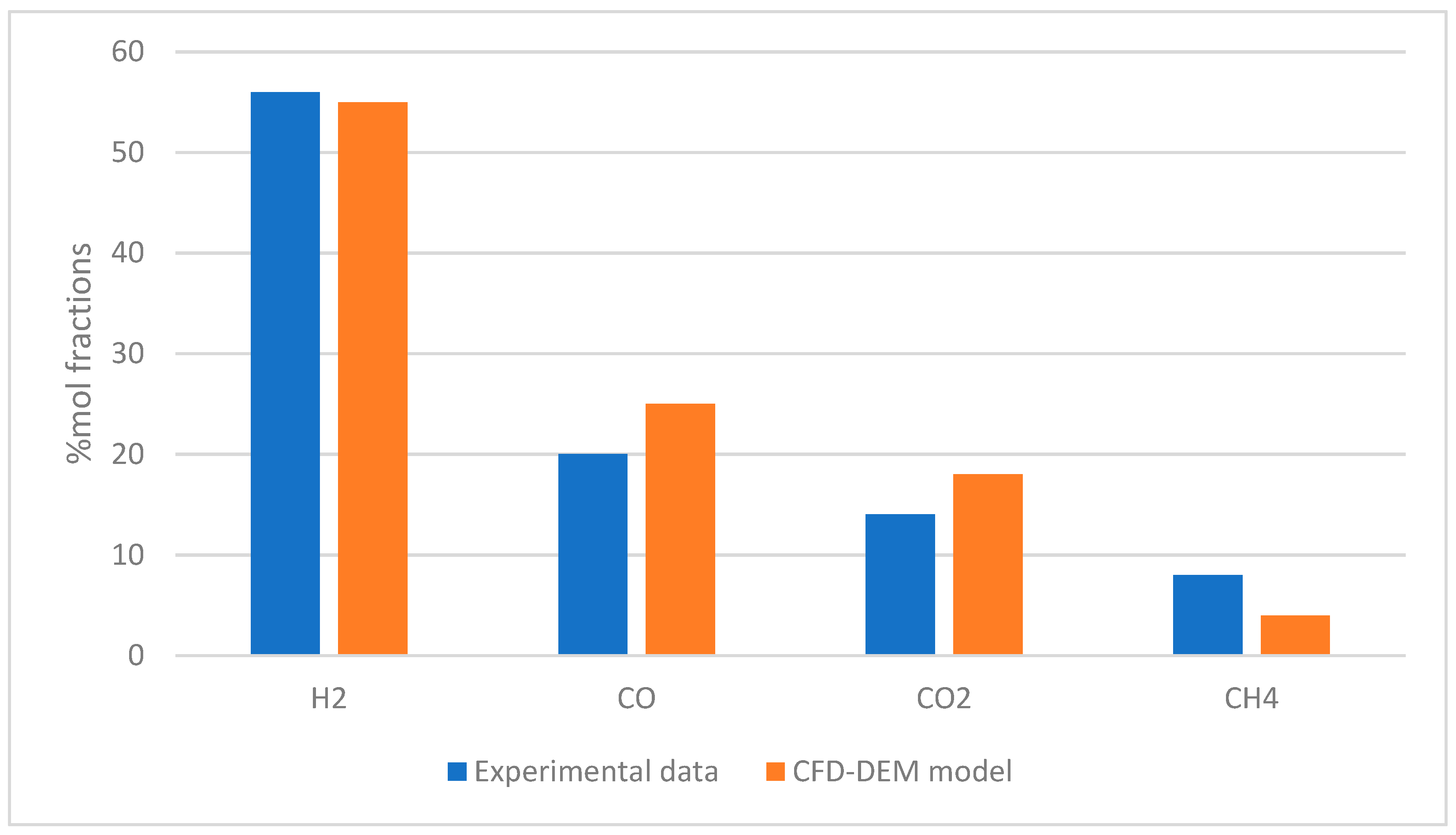

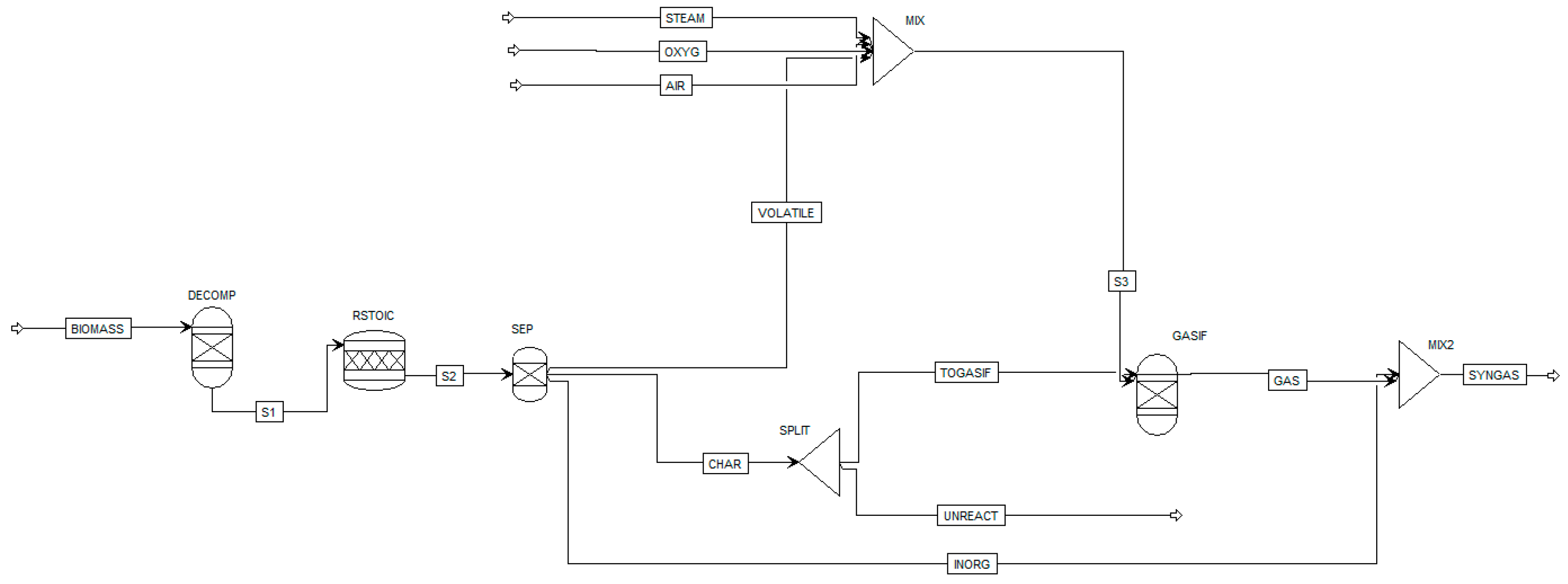
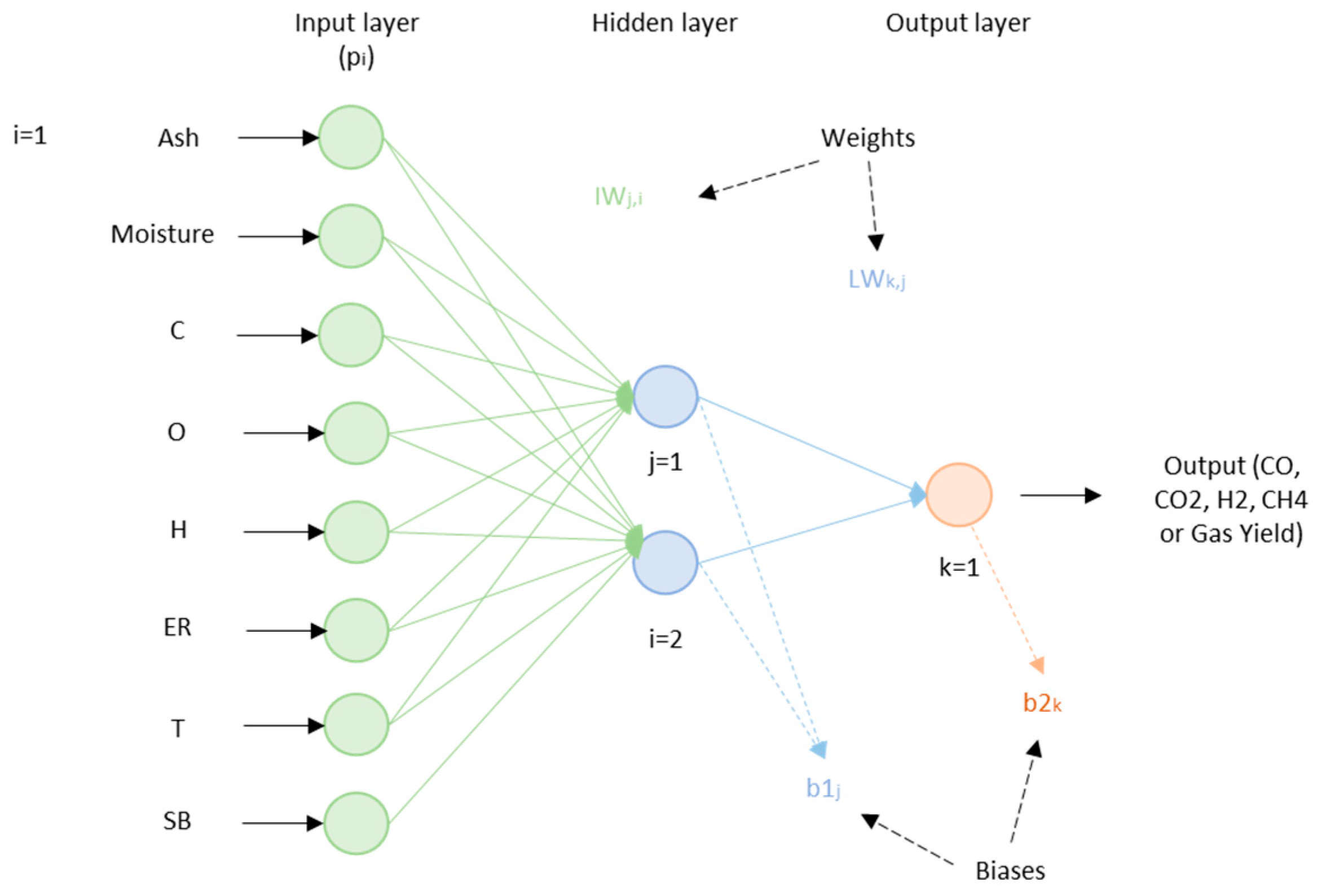

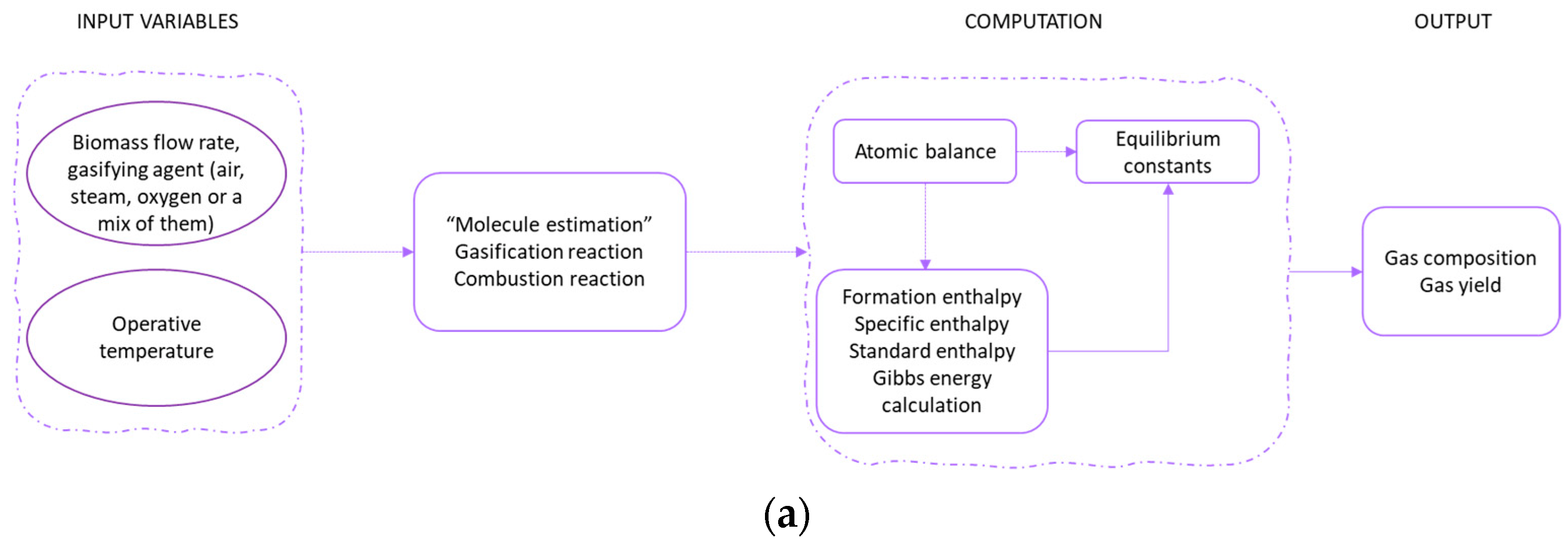
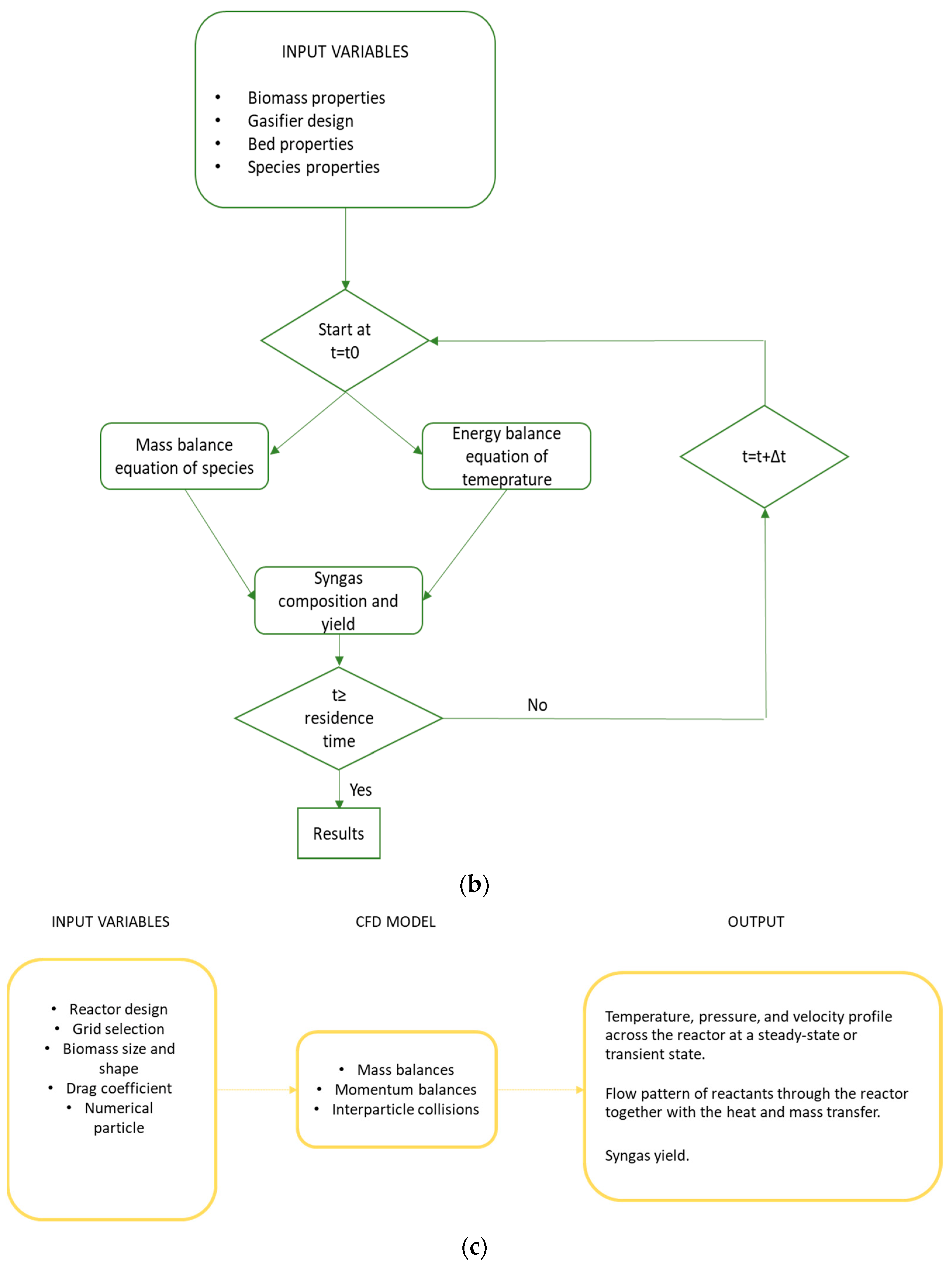


Disclaimer/Publisher’s Note: The statements, opinions and data contained in all publications are solely those of the individual author(s) and contributor(s) and not of MDPI and/or the editor(s). MDPI and/or the editor(s) disclaim responsibility for any injury to people or property resulting from any ideas, methods, instructions or products referred to in the content. |
© 2023 by the authors. Licensee MDPI, Basel, Switzerland. This article is an open access article distributed under the terms and conditions of the Creative Commons Attribution (CC BY) license (https://creativecommons.org/licenses/by/4.0/).