Article

Real-Time Implementation of Sensorless DTC-SVM Applied to 4WDEV Using the MRAS Estimator

1
Laboratoire des Sciences et Techniques Pour l’Ingénieur (LASTI), National School of Applied Sciences (ENSA), Université Sultan Moulay Slimane, Khouribga 25000, Morocco
2
Laboratoire des Systèmes Electriques, Efficacité Energétique et Télécommunications (LSEEET), Faculty of Sciences and Technologies, Université Cadi Ayyad, P.O. Box 549, Marrakech 40000, Morocco
3
Laboratoire Systèmes Electrotechniques et Environnement (LSEE), Université Artois, UR 4025, F-62400 Béthune, France
*
Author to whom correspondence should be addressed.
Energies 2023, 16(20), 7090; https://doi.org/10.3390/en16207090
Submission received: 14 August 2023 / Revised: 20 September 2023 / Accepted: 25 September 2023 / Published: 14 October 2023

Abstract

:
This article presents the DTC-SVM approach for controlling a sensorless speed induction motor. To implement this approach, a practical prototype is built using a microcontroller, an embedded GPS module, and a memory card to collect real-time data during the driving route, such as road geographical data, speed, and time. These data are then utilized in the laboratory to implement the control law (DTC-SVM) on the electric vehicle. The d-q model of the induction motor is first presented to explain the requirements for calculating the rotor speed. Then, an adaptive model reference system speed estimator is developed based on the rotor flux, along with a controller and DTC-SVM strategy, which are implemented using the dSpace 1104 board to achieve the desired performance. The simulation results demonstrate satisfactory speed regulation with the proposed system. In this study too, an electronic differential system is modeled for the four wheels of an electric vehicle equipped with an integrated motor, all controlled by the DTC-SVM strategy. Vehicle speed and electrical vehicle steering angle variations, as well as wheel speeds estimated by code system, are verified using MATLAB/Simulink simulations.

1. Introduction

Energy and environmental issues are now major concerns at the international level. The industrial activity of emerging economic powers has led to an explosion in energy needs. For this reason, several research efforts have been conducted on electric vehicles (EVs) to mitigate the greenhouse effect and its impact on global warming.
The field of control for AC machines continues to evolve due to the demands of industrial operations. The induction motor (IM), owing to its low cost and robustness, is currently the most widely used for numerous applications (e.g., variable-speed operations).
In fact, the IM presents a significant difference compared to the direct current machine. In the case of the IM, the power is supplied through a single winding, which means that the same current creates both the flux and the torque. Consequently, torque variations lead to flux variations, making the control model more complex than in the case of the direct current machine.
The scalar control, while well suited for certain types of drives, does not allow controlling the IM effectively during transient conditions and at low speeds. It is no longer suitable for achieving precise positioning of the IM.
The development of power electronics and digital electronics has contributed to the development of more advanced control algorithms that improve the static and dynamic performance of this type of motor. This advancement allows for the decoupling of flux and torque, enhancing the overall performance of IM [1].
There are essentially two methods of flow control: the first is direct, which is based on closed-loop control, and the second is indirect, characterized by open-loop flow control.
The field-oriented control (FOC) was developed to eliminate internal machine coupling. However, while it provides high performance for the IM, the FOC by rotor flux orientation has some disadvantages:
  • Low robustness to variations in rotor parameters;
  • Presence of coordinate transformations that depend on an estimated angle;
  • Use of a mechanical sensor (fragile and costly). When not using this sensor (Sensorless drive), the machine’s performance is degraded.
Direct torque control with space vector modulation (DTC-SVM) is indeed a control technique used in electric motor drives, particularly in IM drives, to achieve precise control of torque and flux. It combines the principles of DTC with SVM to provide more efficient and precise control of motor parameters [2,3]. It provides recognized benefits compared to traditional methods, especially in terms of reducing the time it takes to respond to torque changes, enhancing resilience to variations in rotor parameters, minimizing DTC and stator flux ripple amplitudes, and eliminating the need for Park transformations. Moreover, this torque control algorithm naturally adjusts to the absence of mechanical sensors, such as speed and position indicators.
Sensorless control has garnered significant interest over the past few decades, both within the realm of research and experimental applications. This method has the potential to reduce hardware complexity, costs, and the physical footprint of control equipment. It eliminates the need for sensors, thereby improving motor control efficiency and reliability, enhancing noise resistance, bolstering overall reliability, and reducing maintenance requirements [4,5].
Literature is rich with works concerning the field of estimators, and the model reference adaptive system (MRAS) techniques have been proven to be one of the best techniques proposed by researchers. This is due to the excellent performance it exhibits in terms of reliability, stability, and reduced computational efforts [4,5,6].
MRAS methods are based on a comparison between a reference model and an adaptation model. The output error is used to drive a suitable adaptation mechanism that generates information about the rotor speed. However, the use of these methods is limited by parametric variations [7,8].
In the literature, there are also stochastic approaches like the Kalman Filter, which are very effective in obtaining highly accurate estimations. Additionally, adaptive approaches based on observers can also be found, characterized by their adaptive mechanisms that ensure velocity estimation. On the other hand, methods based on artificial intelligence, such as neural networks and genetic algorithms, can achieve high performance. However, these algorithms are relatively complex and require powerful computational resources [9,10].
The authors of [11,12] presents DTC-SVM by applying fuzzy logic to the IM. This approach involves substituting hysteresis controllers and the selection table to achieve fuzzy DTC control. This substitution ensures a reduction in switching losses and an enhancement in dynamic performance. They operated the IM at a constant switching frequency using SVM based on the three nearest vectors instead of hysteresis controllers, which can provide acceptable control performance using a sensorless algorithm for accurate estimation. Consequently, implementing DTC-SVM control using hysteresis controllers improves control performance and enhances system reliability by reducing sensor usage costs in EVs.
To demonstrate the effectiveness of the proposed new control strategy on the four-wheel drive electric vehicle (4WDEV) traction system, a traction system consisting of four 1.5 kW IM mounted on the wheels was used, driving both the rear and front wheels. The speed of each IM is independently calculated during turns using a differential system. Four proportional-integral (PI) speed controllers are used to recalculate the reference torque for each wheel’s electric motor (EM) based on driving requirements. The EV has been tested on two different road. Simulation results demonstrate the vehicle’s stability during both driving cycles.
The main advancements of this research include, firstly, the design of an experimental platform based on a microcontroller and an integrated GPS module, allowing for the collection of location data from real-world trajectories. It will facilitate tasks in the validation of control algorithms for EV on real-world routes. Secondly, the application of the SVM-DTC method, accompanied by the development and testing of an electronically controlled differential specifically designed for 4WDEV in various driving scenarios, this platform demonstrates high performance when subjected to various verification tests for EV.
The organization of this paper can be outlined as follows: The first section introduces the electric powertrain, its description, and modeling. It also includes details on an experimental setup used to collect data from actual trajectories. The second section illustrate the simulation and application of sensorless DTC-SVM to IM. The technique is simulated and executed using the dSpace 1104 platform across various reference speed scenarios. Section three is focused on developing and simulating the electronic differential system, as well as carrying out its real-world implementation on a real trajectory. Finally, section four summarizes the conclusions and future prospects of the work presented in this paper.

2. Electric Vehicle Powertrain

2.1. Electric Vehicle Diagram

2.1.1. Principle

This section presents the model and description of the main components of the proposed electric traction system in this work. Figure 1 shows the diagram of the electric traction system, which can be subdivided into electrical/electronic and mechanical parts. The IM is part of both sections, as this device performs the conversion of electrical energy into mechanical energy.
An EV is a vehicle whose propulsion is powered by an electric motor running exclusively on electrical energy. In other words, the driving force is transmitted to the wheels by one or more electric motors, depending on the chosen transmission solution. The electric propulsion system (Figure 1) is the main component of an EV, which is electrically powered by motors and includes a transmission system consisting of one or more electric motors driving two drive wheels [13].

2.1.2. The Battery

The battery is considered an ideal energy source, meaning it provides optimal performance to ensure adequate power supply to the converter.
There are several types of batteries, but for current EV, Lithium-Ion batteries are frequently used [10,14].
A traction battery must meet the following conditions:
-
High specific power to ensure good vehicle acceleration;
-
A large number of charge/discharge cycles without significant performance degradation;
-
Reduced production cost;
-
Application safety;
-
Fast recharging;
The state of charge (SOC) is estimated by integrating the current [15]:
S O C t = S O C 0 + 1 C i d t
With: S O C 0 et S O C t is the values of SOC are, respectively, the initial and current states. Equation (2) provides the voltage of a battery cell. For a battery pack consisting of N b a t t elements connected in series, the total voltage is:
U b a t t S O C , I b a t t = V b a t t S O C , I b a t t . N b a t t

2.1.3. The DC-AC Converter

The electrical energy converter used in the traction chain is a two-level voltage source inverter (VSI). The three-phase voltage source inverter enables the exchange of energy between a direct voltage source and a three-phase load (stator windings of the induction machine).
The output voltage space vector (Us) of the inverter depends on the value of Ud and the modulation signals Sa, Sb, and Sc.

2.1.4. The Induction Motor

The three-phase IM, which is used to obtain its model, is represented in Figure 2. It shows the three stator phases As, Bs, and Cs, as well as the three equivalent rotor phases Ar, Br, and Cr. θr is the angular position of the rotor, and ωr is the angular velocity of the rotor.

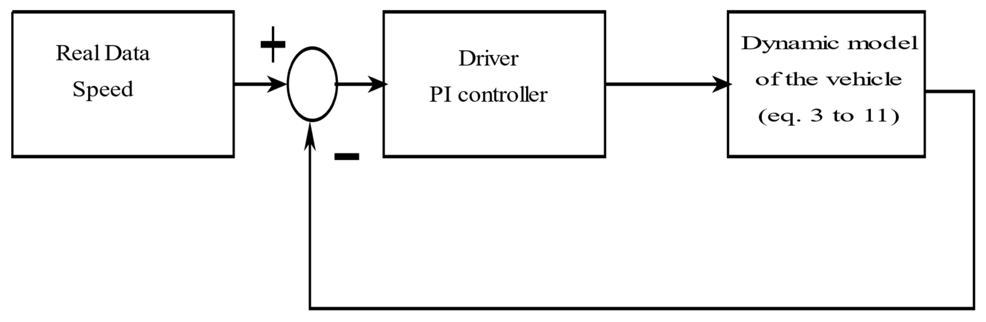
2.2. Dynamic Modelling of the Vehicle

The vehicle is considered as a moving point solid, subject to three forces along the longitudinal axis (Ox) illustrated (as shown) in Figure 3.
Equation (3) is based on Newton’s law applied to vehicles on a road with slope α. As stated in [14,16,17].
  • F t r : the force generated by the powertrain;
  • F a e r : The aerodynamic friction force;
  • F r r : The force of wheel friction;
  • F g : The force of gravity when driving on non-horizontal roads.
F t r t = M v e h a v e h ( t ) + F a e r t + F r r t + F g ( t )
F a e r t = 1 2   ρ S C x V v e h 2 F r r t = M v e h g C r ( V v e h ( t ) ) cos ( α t ) F g t = M g s i n ( α t ) ,
The coefficient C r ( V v e h ( t ) ) is given by the following equation [18];
C r V v e h t = C r 0 + K C r V v e h 2
The coefficients C r 0 and K C r are determined experimentally.
The mechanical power required for the wheels to move or brake the vehicle is given by the product of the forces applied to the vehicle and its instantaneous velocity.
P m t = M v e h a v e h t + F a e r t + F r r t + F g t v ( t ) v e h
The power, P m o t , required by the electrical machine depends on its rotational speed, ω m o t , and its torque, Tmot.
P m o t t = ω m o t t T m o t t η r e d ω m o t t T m o t t s i g n ( T m o t t )
The gearbox adapts the speed and torque between the electric machine shaft ( ω m o t , C m o t ) and the drive wheels ( ω w h e e l , C w h e e l ).
The transmission primarily consists of the differential block, tasked with evenly distributing the output torque from the gearbox to the driving wheels. An overall reduction ratio is considered between the electric machine shaft and the wheel. It is assumed that the efficiency of the gearbox/transmission assembly remains constant. Based on these assumptions, the relationships between torques and speeds are provided as follows:
T m o t t = T w h e e l t η r e d ( s i g n C m o t t ) r r e d
ω m o t t = ω w h e e l t r r e d
ω w h e e l t = V v e h ( t ) R w h e e l
The relationship between the linear velocity of the vehicle,   V v e h , and the rotational speed of the wheel,   ω w h e e l , is given by:
ω w h e e l t = V v e h ( t ) R w h e e l

2.3. Experimental Test

The experimental model installed in the vehicle (Figure 3) consists mainly of a microcontroller, a GPS module, a timmer, and a memory card. This setup allows for the collection of geographical data from the road in accordance with the vehicle’s speed. These data are compiled in Table 1 [19]. The data obtained from the practical experiment in Figure 4 is confirmed by the itiner-ary illustrated in Figure 5.
The trajectory data used are real data from the Safi to Rabat highway in Morocco, collected by the model in Figure 4 using onboard GPS. Table 1 presents all the data recorded on a memory card and is utilized in the laboratory for conducting tests on EV control.
Table 1. Recorded data from the Safi–Rabat road.
LatitudeLongitudeAltitude (m)Speed (Km/h)Time/Date
32.35699−9.274521113.9015:20:53/13 May 2022
32.36787−9.273886113.928.515:21:08/13 May 2022
32.3784−9.273513113.728.515:21:24/13 May 2022
……….……….……….……….……….
……….……….……….……….……….
……….……….……….……….……….
33.98274−6.94468770.895.419:25:30/13 May 2022
33.9849−6.94456272.570.819:25:48/13 May 2022
33.98707−6.94021873.691.319:27:05/13 May 2022
Figure 5. The itinerary between Safi and Rabat in Morocco.
Energies 16 07090 g005

2.4. Simulation Results and Discussion

Figure 6 provides a representation of the closed-loop schematic for the dynamic model of the EV, which employs a PI controller. Meanwhile, Figure 7 showcases the results of simulations conducted in the Matlab/Simulink environment, utilizing real data collected by the embedded system depicted in Figure 4. These simulations were conducted during the EV’s operation on the SR itinerary outlined in Figure 5, which is situated in Morocco.
The results obtained with the model shown in Figure 7 are provided for a Berlingo-type vehicle equipped with a 40 kW fuel cell system (FCS) and a set of 200 Nickel-Metal Hydride (Ni-MH) battery elements. The SR cycle (Moroccan Cycle) and FTP75 cycle (European Normalized Cycle) are considered.
The data of the vehicle used in the simulation are grouped in Table 2.
The PI controller is used to track the setpoint within an allowable maximum error. This controller operates on the dynamics of the closed-loop system, thus affecting consumption performance.
The control strategy does not take into consideration the SOC of the batteries to calculate the power distribution, which means there is no guarantee of its performance over a longer cycle. Clearly, it is necessary to implement more appropriate strategies that minimize one or several criteria, for example, the SOC of the battery, while respecting a set of constraints (such as limited power, etc.).
  • Scenario 1: SR Route (Safi–Rabat).
Figure 7. Vehicle simulation results, (a) Speed response; (b) Wheel torque; (c) Power transmitted to the wheels; (d) Motor torque.
Energies 16 07090 g007
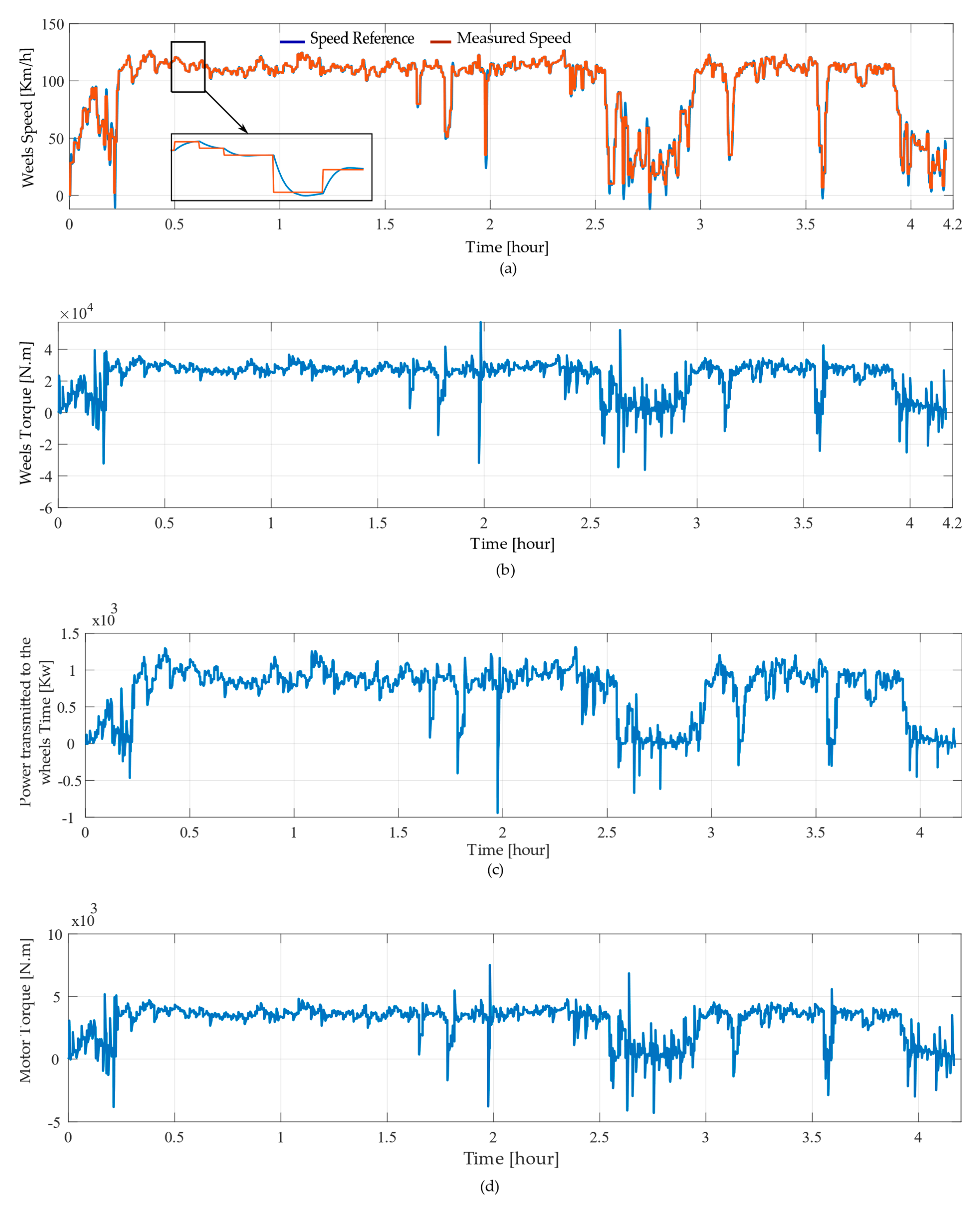
  • Scenario 2: Driving cycle FTP75.
The FTP75 route is a standardized road used by EV designers. The profile of this route is depicted in Figure 8.
Figure 8. Vehicle simulation results, (a) Speed response; (b) Wheel torque; (c) Power transmitted to the wheels; (d) Motor torque.
Energies 16 07090 g008
The following section will be devoted to the study and control of IM. The most significant advantage of IM is that their speed can be easily adjusted by changing the power frequency. This characteristic makes them highly compatible with EVs.

3. Direct Torque Control Modeling

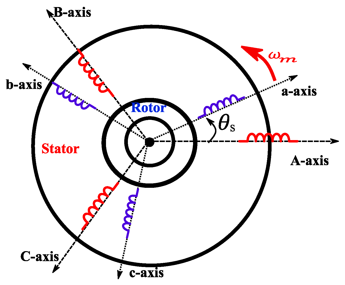
3.1. Induction Motor Modeling

To establish the controls applied to the IM of the EV, the model is calculated using the Concordia transformation ( α β ). This allows us to have a reduced and simplified model expressed by the following expressions [20,21,22]:
  • Electrical equations:
v s α = R s i s α + d φ s α d t v s β = R s i s β + d φ s β d t v r α = R r i r α + d φ r α d t + ω m φ r β v r β = R r i r β + d φ r β d t ω m φ r α
  • Magnetic equations:
φ s α = L s i s α + L m i r α φ s β = L s i s β + L m i r β φ r α = L r i r α + L m i s α φ r β = L r i r β + L m i s α
  • Mechanical equations:
T e m = φ s α i s β φ s β i s α J d Ω d t + f Ω = T e m T r

3.2. Two-Level Voltage Source Inverter Modeling

Figure 9 illustrates the voltage inverter that is composed of three legs, each having two complementary switches based on IGBT transistors. The control of these switches is ensured by various modulation techniques.
The mathematical model of the two-level voltage inverter is represented by the following matrix:
v a v b v c = V d c 3 2 1 1 1 2 1 1 1 2 s a s b s c
The state of the switches is assumed to be ideal and can be represented by three Boolean variables of the control: Sa, Sb, and Sc, such that:
  • Si = 1 if T i is closed and T i ¯ is opened.
  • Si = 0 if T i is opened and T i ¯ is closed.
Where: (i = a, b, c).

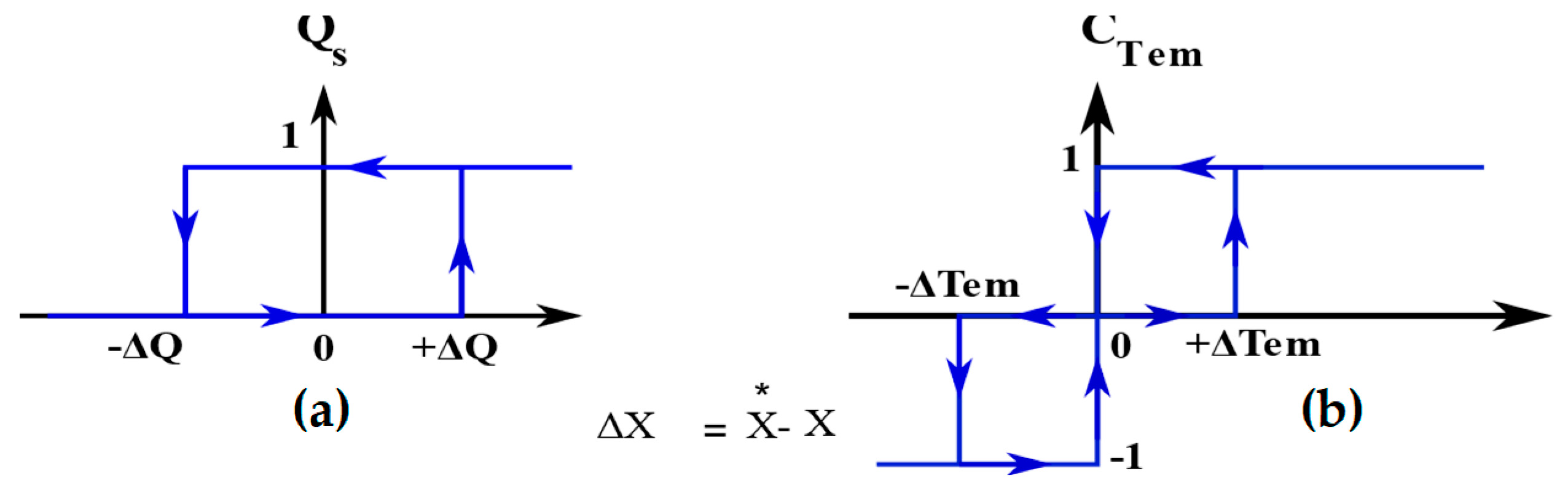
3.3. The DTC-SVM Strategy

This technique retains the basic idea of the conventional DTC technique. The control voltages can be generated by the PI controllers for the stator torque and flux, and implemented using the vector PWM control technique [23,24].
The block diagram of the DTC-SVM control technique applied to the IM is shown in Figure 10. In this structure, regulators calculate the reference voltages in the stationary frame (α-β). The obtained α and β components will then be injected into the SVM block.
The operating principle of this strategy lies in regulating the flow and torque parameters without having direct measurements of these parameters. This is achieved by estimating the flow and torque and comparing them to flow and torque references.
The stator flux vector is estimated based on the measurements of the voltages and currents of the induction motor [25]. The expressions for the stator fluxes are given by:
φ ^ s α = v s α R s i s α d t φ ^ s β = v s β R s i s β d t
The magnitude of the stator flux and the angle related to the stator reference frame are expressed as follows:
φ s = φ s α 2 + φ s β 2 θ s = t a n 1 φ s β φ s α
One of the six voltage vectors of the inverter can be appropriately chosen to control the position and magnitude of the stator flux and indirectly the rotor flux, depending on the variation in the stator flux [26,27,28].
Table 3 shows the different voltage vectors of the inverter that can be applied in a DTC drive.
T ^ e m = 3 2 p ( φ ^ s α i s β + φ ^ s β i s α )
The amplitudes of the stator flux and torque are compared to their respective estimated values, and the errors are treated through hysteresis controllers. The output of the flux and torque comparator is used for the ideal commutation table of the inverter.

3.4. Elaboration of the Switching Table

The switching states of the inverter are determined by torque and flux errors based on the sector determined. In order to maintain the estimated torque and flux within their limits, as indicated by the two hysteresis bandwidths shown in Figure 11a,b, at each sampling period, the torque and flux are estimated and then compared to the corresponding reference values before passing through the comparator. The position of the stator flux and the most suitable spatial vector among those generated by a VSI are selected based on the commutation table provided in Table 3 to compensate for the load torque and stator flux.
Figure 11. (a) Two-level flux controller; (b) Three-level torque controller.
Energies 16 07090 g011
Table 3. Switching Table.
Sector123456
Δ Φ s
Δ T e v 2 v 3 v 4 v 5 v 6 v 1
Δ T e = 0 v 7 v 0 v 7 v 0 v 7 v 0
Δ T e v 6 v 1 v 2 v 3 v 4 v 5
Δ Φ s
Δ T e v 3 v 4 v 5 v 6 v 1 v 2
Δ T e = 0 v 0 v 7 v 0 v 7 v 0 v 7
Δ T e v 5 v 6 v 1 v 1 v 4 v 3

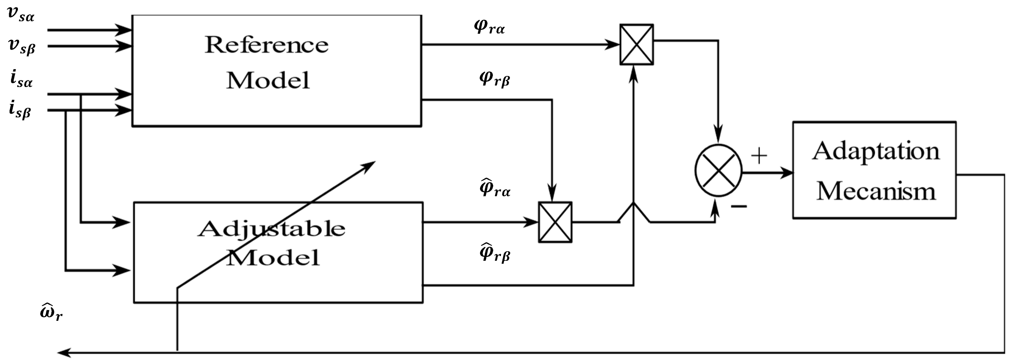
3.5. Design of a Rotor Flux Model Reference Adaptive System Observer

The structure of the Rotor Flux MRAS observer illustrate in Figure 12 consists of two parts: a reference model and an adaptive model that contains the estimated variable (rotor speed). Additionally, there is an adaptation mechanism to update it. The reference model is called the voltage model.
It is expressed by the reference voltages in the steady-state framework and generates the reference flux values. Furthermore, the adaptive model is also known as the current model. It is expressed by the stator currents and the rotor speed. The voltage and current equations are expressed as follows: [29,30,31]:
d φ r α d t = L r L m v s α R s   i s α σ L s d i s α d t d φ r β d t = L r L m v s β R s   i s β σ L s d i s β d t
d φ ^ r α d t = 1 T r L m i s α φ ^ r α ω ^ r φ ^ r β d φ ^ r β d t = 1 T r L m i s β φ ^ r β + ω ^ r φ ^ r α
σ is a leakage coefficient of inductances, where σ = 1 L m 2 L s L r .
The error between the two models is expressed by:
e = φ r β φ ^ r α φ r α φ ^ r β
The observed error between the states of the two models given by Equation (21) is used to generate ω r using a PI controller as an adaptation mechanism.
A simple PI controller allows the estimation of the rotor speed, based on the error between the estimated fluxes from the measurement of stator currents and voltages.
ω ^ r = K p + K i S e
where K p and K i are the proportional and integral gains, respectively.
Figure 12. The model reference adaptive system based on rotor flux.
Energies 16 07090 g012

3.6. Simulation Results

The parameters of the motor used in the simulation are from an IM identified within the laboratory (Table 4):
The simulation of the DTC-SVM is performed using Matlab/Simulink. Figure 13 displays the results of the DTC-SVM simulation in response to a step-speed reference, while Figure 14 presents the DTC-SVM responses to a variable-speed reference.

3.6.1. Speed Step Response

In order to evaluate the performance of the DTC-SVM controller, multiple tests were executed in the MATLAB/SIMULINK environment. Figure 13 illustrates the simulation results obtained when applying a step-speed reference. This approach enables us to analyze the characteristics and effectiveness of the DTC-SVM control strategy.
Figure 13. Simulation results, (a) Real and estimated speed responses with MRAS observer [rpm]; (b) Speed error [rpm]; (c) Stator currents [A]; (d) Estimated torque and its reference [N.m]; (e) Quadrature current Isq [A]; (f) Rotor position θ and θ ^ estimated position; (g) Flux αβ [Wb]; (h) trajectory of flux αβ.
Energies 16 07090 g013

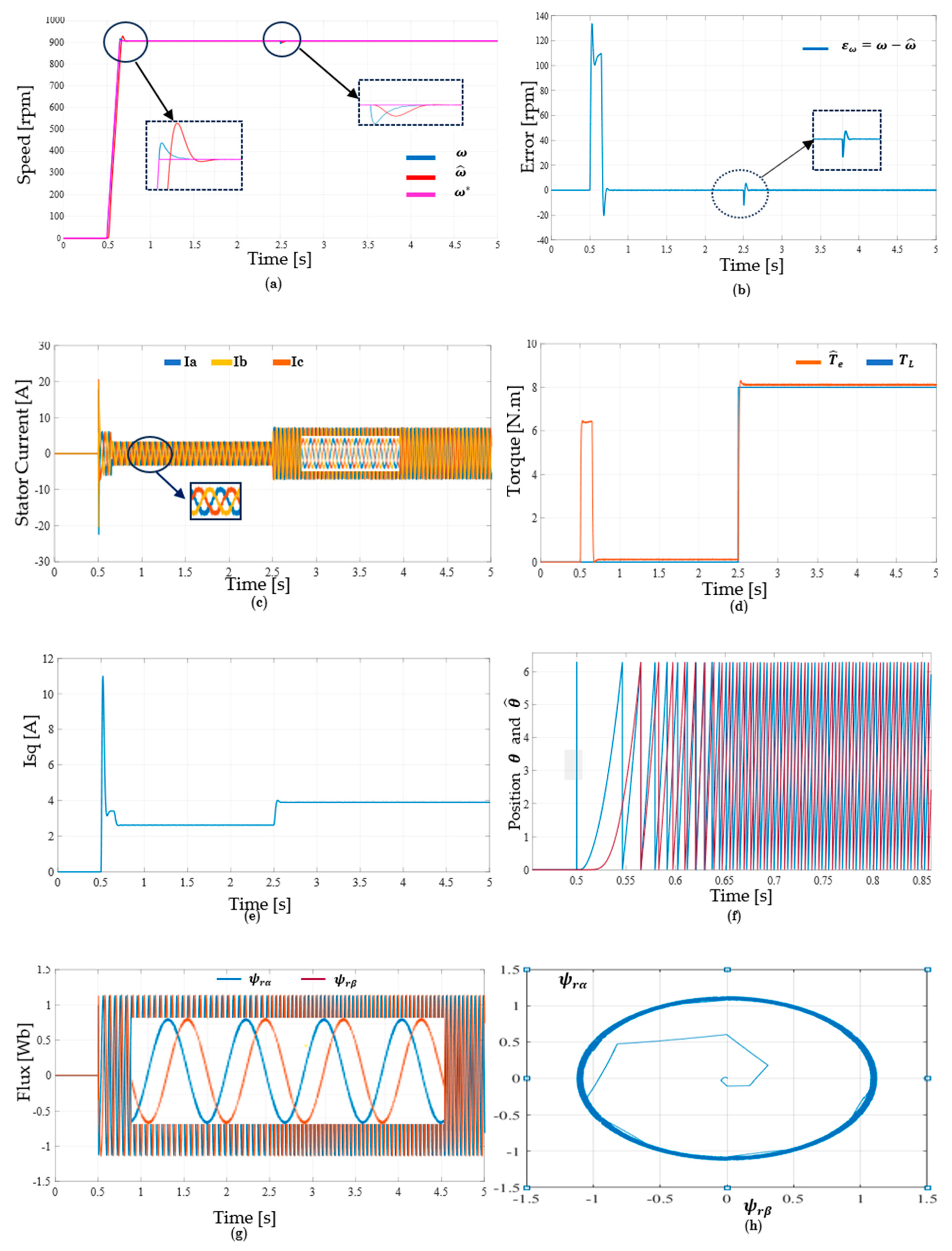
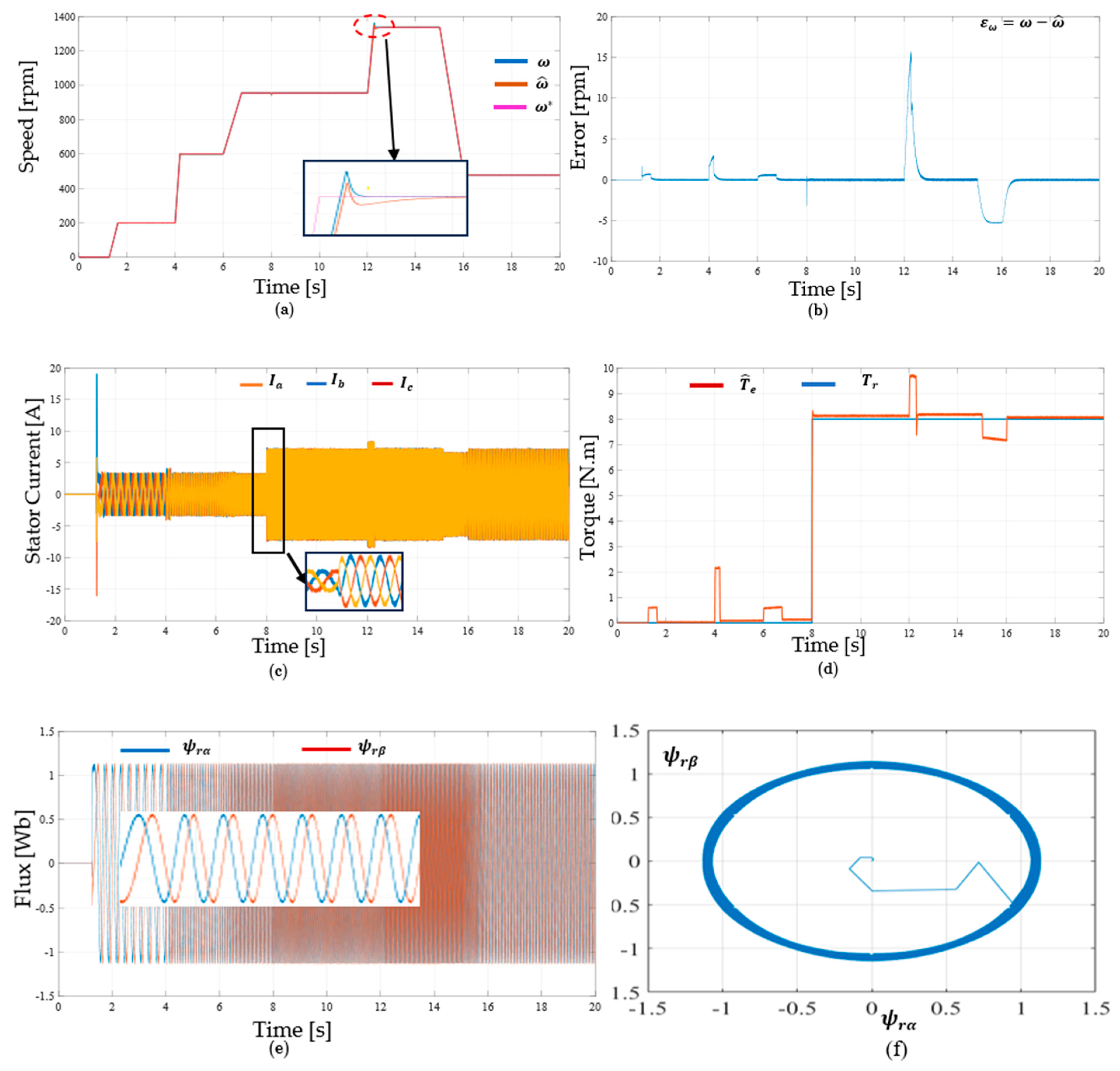
3.6.2. Variable Speed Response

Figure 14 displays the simulation results after brusquely changing the speed setpoint. These tests were conducted using the Matlab/Simulink environment, allowing us to evaluate the ability of the DTC-SVM approach to maintain its performance in the presence of disturbances.
Figure 14. Simulation results, (a) Measured and estimated speed responses with MRAS observer [rpm]; (b) Speed error; (c) Stator currents [A]; (d) Estimated torque and its reference [N.m]; (e) Flux α β [wb]; (f) trajectory of flux α β .
Energies 16 07090 g014

3.7. DTC-SVM Control Implementation

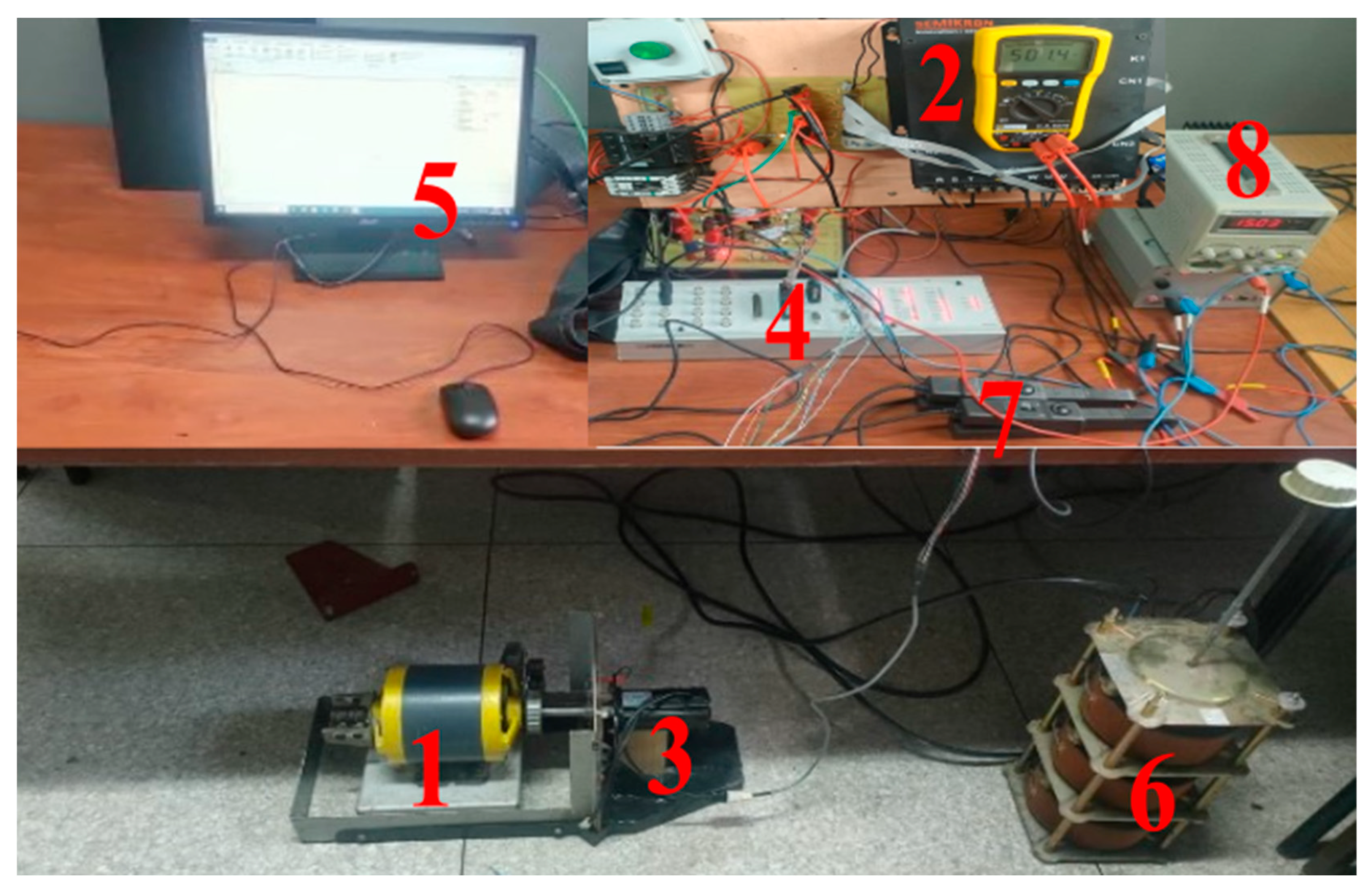
3.7.1. Experimental Test Bench

The DTC-SVM control developed in this work is implemented in real-time using the dSpace 1104 system. The real-time interface serves as a link between dSpace 1104 and MATLAB/Simulink software. The power circuit of the drive consists of an industrial inverter.
The motor used in this experimental study is a three-phase IM, and it is controlled by DTC-SVM under load. Figure 15 shows the experimental setup diagram of the platform used.
The practical test bench consists of the following elements:
1: A squirrel-cage IM;
2: A power electronics Semikron converter composed of a rectifier and an IGBT inverter;
3: A speed sensor (incremental encoder), used in order to check and compare the real speed with the estimated speed;
4: A Dspace 1104;
5: Control desk software plugged into a personal computer;
6: An autotransformer;
7: A currents sensor;
8: A DC power supply;
Figure 16 illustrates the components necessary for conducting experimental tests. In this context, a conventional low-power and low-torque laboratory motor is typically employed. Nevertheless, it’s important to adapt the utilization of conventional IM to meet the power demands of EVs. Conventional IMs designed for EV applications present several benefits, including improved efficiency, cost-effectiveness, durability, and reliability. Consequently, they represent a practical and significant choice to contemplate when designing and producing electric vehicles.

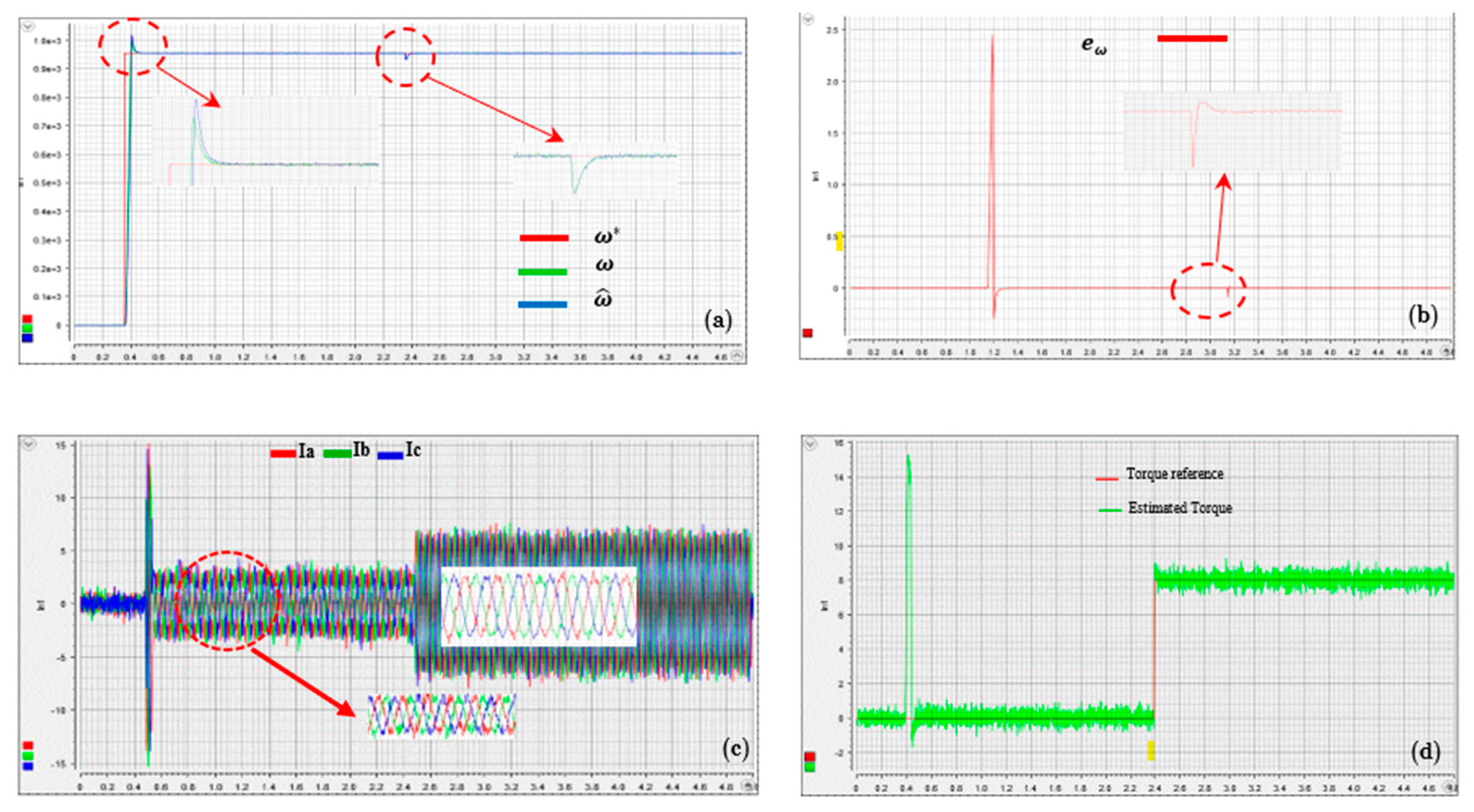
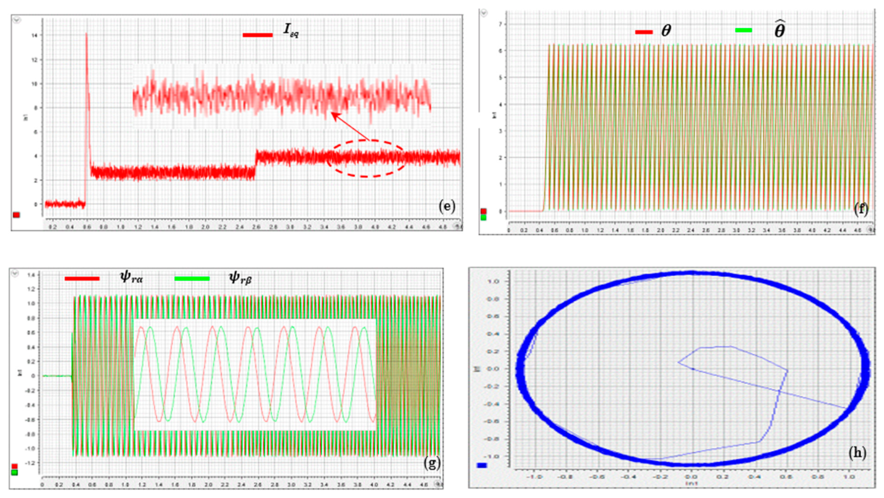
3.7.2. Experimental Results

The proposed control scheme, which was implemented in MATLAB/Simulink, is also verified through experimental tests. Real-time control was performed in the laboratory equipped with a dSpace 1104 card.
This test is conducted by introducing a load torque TL = 8 Nm after an empty start at t = 2.5 s. Figure 17 shows the responses of the IM variables while maintaining a constant reference speed. The effects of the load do not have any influence on its rotation speed. The load torque and the change in rotation speed do not affect the two components of the rotor flux.

4. Electronic Differential System

4.1. The Electronic Differential System

The electronic differential system (EDS) for EV with four independent motors in the wheels is indeed a highly complex control system. Figure 18 illustrates the proposed structure of the electronic differential, where the front left and right wheels, as well as the rear left and right wheels, are controlled by four individual wheel motors. IMs are preferred for their high efficiency, high torque density, quiet operation, and their suitability for EV applications [32].
In Figure 18, X α β represents the reference speeds of the four engines generated by the EDS system, such as α β =  [rf, lf, rr, lr]
Figure 18. Proposed electronic differential.
Energies 16 07090 g018
In this study, the model presented in Figure 19 is preferred for the design of the (EDS). This model establishes the relationship between the inner and outer wheels on a curved road. Tires are not considered in this model. Some parameters such as the road curvature radius, vehicle speed, distance between the front and rear wheels, steering angle, and distance between the rear wheels are included in the model. The characteristics outlined in Table 5 are determined through the following calculations:
A position encoder serves the purpose of monitoring the steering angle of the electric vehicle (EV). When the steering angle reads as zero, it indicates that the EV is traveling in a straight line along the road. Conversely, if the steering angle deviates from zero, it signifies that the EV’s wheels are being turned either to the left or the right. In this case, it is essential for the speed of the inner wheel to be lower than that of the outer wheel, aligning with the direction of the turn.
Figure 19. Kinematic model of four-wheel drive electric vehicle.
Energies 16 07090 g019
The dynamics of each wheel drive system can be expressed as follows:
J x y d X x y d t = T e x y F x y ω x y T r x y x y = r f , l f , r r , l r
where J x y , and F x y are the torque and friction coefficient for each respective motor, and the abbreviations r f , l f , l r , and r r stand for the right front, left front, left rear, and right rear, respectively.
Each motor is equipped with a fixed-ratio gear reducer, which is attached to the wheel, forming a driving wheel.:
  ω w h e e l x y = X x y k g e a r T w h e e l x y = T e x y k g e a r η t
where η t is the transmission efficiency, and k g e a r is the gearbox coefficient.
Table 5. Definition of parameters in kinematic mode.
ω v e h Vehicle reference speed
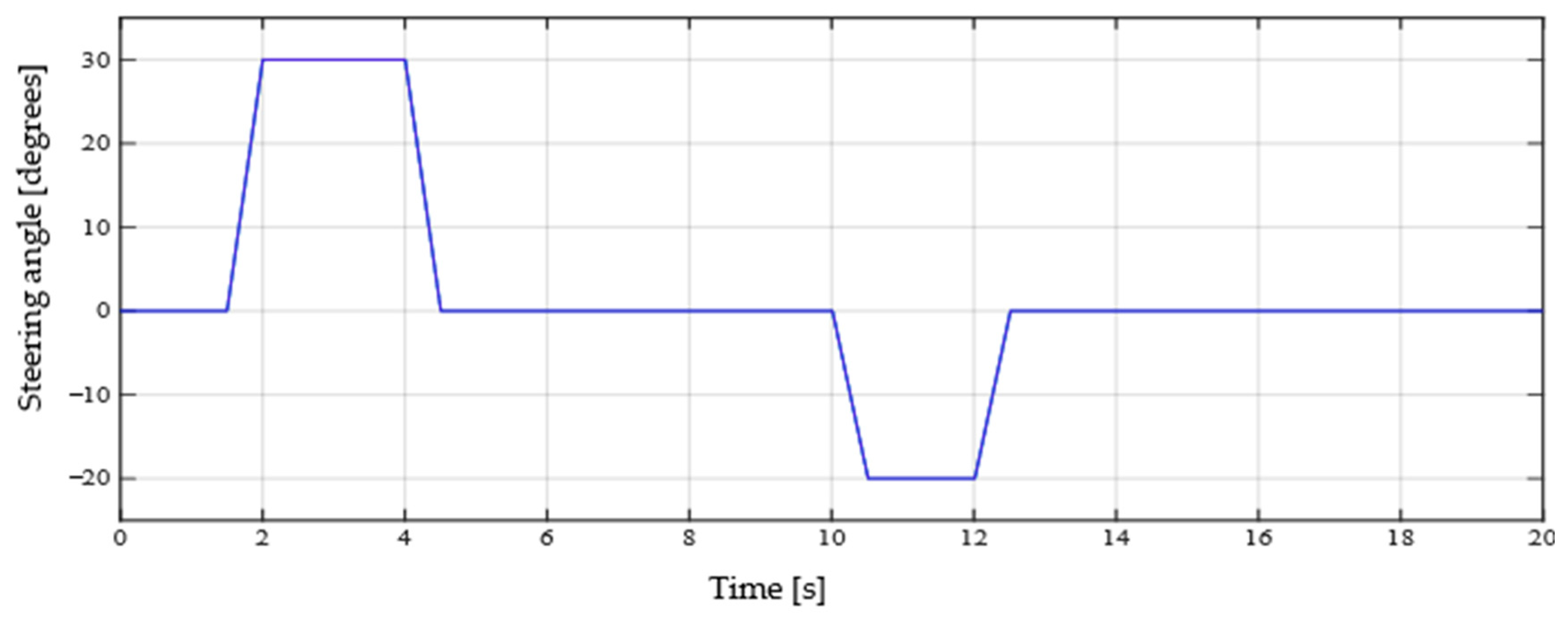
δ Steering angle (°)
δ 1 Turning angle of left front wheel (°)
δ 2 Turning angle of right front wheel (°)
L ω Length of vehicle (m)
d ω Width of vehicle (m)
R Steering radius of center of rear axle
R 1 Steering radius of inside rear wheel
R 2 Steering radius of outside rear wheel
r Steering radius of center of front axle
r 1 Steering radius of inside front wheel
r 2 Steering radius of outside front wheel
v l f ,   v r f Linear speed of left front in wheel and right front in wheel
v l r ,   v r r Linear speed of left rear in wheel and right rear in wheel
R = L ω t a n ( δ ) R 1 = R d ω 2 R 2 = R + d ω 2
r = L ω 2 + R 2 r 1 = L ω 2 + R 1 2 r 2 = L ω 2 + R 2 2 r = L ω 2 + R 2 r 1 = L ω 2 + R d ω 2 2 r 2 = L ω 2 + R + d ω 2 2
The angular velocities of the two front and rear driving wheels are given by:
    ω l f = ω v e h   1 + cot δ d w 2 L w   2 1 + cot δ 2     ω r f = ω v e h   1 + cot δ + d w 2 L w   2 1 + cot δ 2     ω l r = ω v e h   1 d w tan δ 2 L w ω r r = ω v e h   1 + d w tan δ 2 L w
According to Equations (26) and (27), the reference speed for the four induction wheel motors is expressed as:
X l f = k g e a r . ω l f X l r = k g e a r . ω l r X l r = k g e a r . ω l r X r r = k g e a r . ω r r

4.2. Speed Controller Design of IM Drive

The ED algorithm produces the speed references X l f , X l r ,   X l r ,   a n d   X r r for the front and rear motors of the inner wheels. The reference speed and the actual speed of each free-wheeling motor are inputs to the speed controller blocks. The closed-loop speed controller generates the reference motor torque T e _ x y .

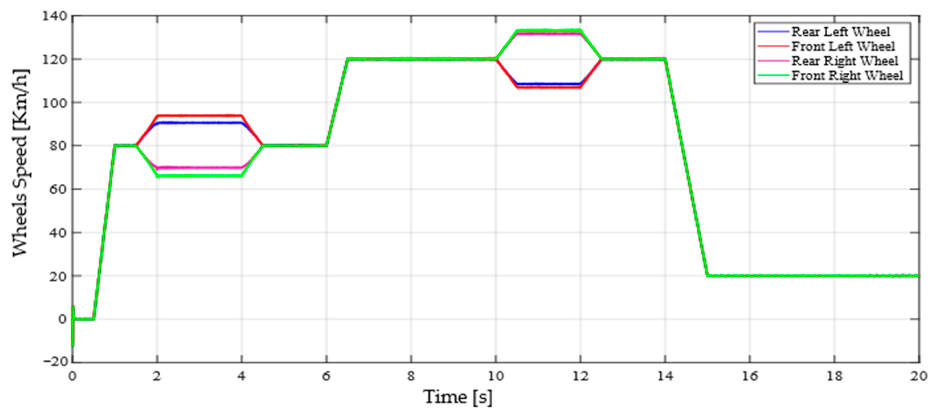
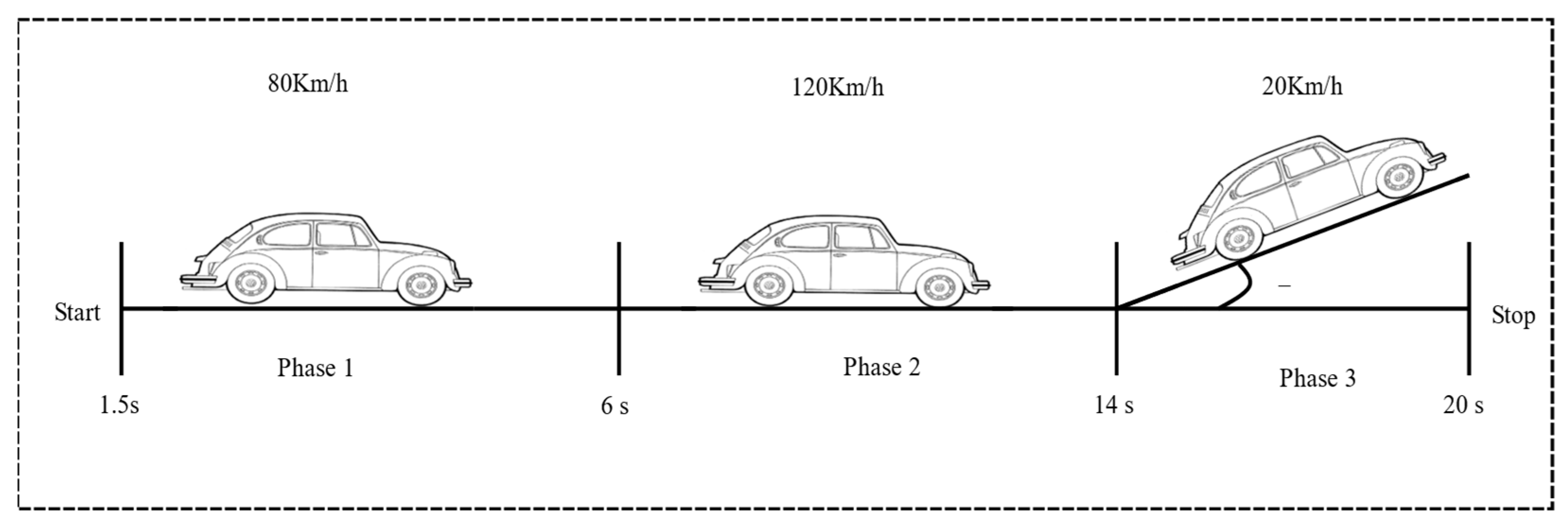
4.3. Vehicle Speed Profile

The speed profile chosen to perform the simulation of the electronic differential system for the EV is developed in Figure 20. This trajectory is defined by three phases. Table 6 provides more details.

4.4. Simulation Results

To confirm the effectiveness of the DTC-SVM control strategy on the 4WDEV traction system, the system was subjected to a change in the reference speed according to the Marrakech-Safi trajectory structure developed in Section 2.3.
At the current level, the driver imposes two turns on the vehicle chassis using the steering angle. The first turn is executed to the right (Phase 01) at t = 1.5 s, while the second turn is executed to the left at t = 10 s. Figure 21 presents the front vehicle steering angle curve as specified by the driver. A positive value of the steering angle (δ = 30°) corresponds to a right turn, while a negative value (δ = −20°) corresponds to a left turn. Figure 22 shows the linear velocity of each wheel when the turns are made at a constant speed. The driver provides a desired steering angle δ* that is initially applied to the front wheels’ steering angle.
The EDS immediately acts on all four IM of the wheels, individually adjusting the speed of each wheel. When a right turn is executed, the electronic differential decreases the speed of the two wheels located on the inside of the turn while increasing the speed of the two wheels located on the outside of the turn. During the first control phase (Phase 01), it is observed that the two front and two rear wheels located on the outside of the right-curved turn rotate at higher speeds than the two wheels on the right side (front and rear). Similarly, it is noticed that the two right front wheels and the two left rear wheels rotate at higher speeds than the two wheels on the left side during the right turn. Figure 22 effectively illustrates the speed difference between the four wheels during vehicle turning.
Figure 22. Variation in speed of the four wheels in different phases.
Energies 16 07090 g022

5. Conclusions

This article outlines a comprehensive approach to modeling an EV in a real-world route. It begins with the development of dynamic model and proceeds to the practical implementation of this model in a prototype. The primary objective is to assess motor power, torque, and power transmission to the wheels. The process involves utilizing machine equations and an equivalent stator circuit, leading to the creation of a Direct Torque Control algorithm with Space Vector Modulation (DTC-SVM). This algorithm maintains a constant ratio between the SVPWM switching frequency and the fundamental supply frequency. The DTC-SVM algorithm is then implemented on the dSpace 1104 board to validate the simulation results. The aim is to draw conclusions regarding the qualities and drawbacks of this control method while suggesting enhancements to enhance the electric vehicle’s range. Furthermore, the modeling and simulation of the 4WDEV electric vehicle using the DTC-SVM technique are conducted on an actual trajectory, taking into account various constraints such as acceleration, deceleration, and road conditions. An important observation emerges: when the inner wheel’s speed of the electric vehicle decreases, the outer wheel’s speed increases due to the steering angle’s expansion. The speeds of the front wheels are estimated using the Codesys algorithm, and all these findings are corroborated using Matlab/Simulink. In conclusion, this study demonstrates that employing DTC-SVM control for the induction machine yields significant benefits, including dynamic control, optimized performance, enhanced robustness, and reduced computational load.

Author Contributions

Conceptualization, A.B. (Abdelhak Boudallaa) and M.C.; methodology, A.B. (Abdelhak Boudallaa), A.B. (Ahmed Belkhadir) and M.C.; software, A.B. (Abdelhak Boudallaa), A.B. (Ahmed Belkhadir) and M.C.; validation, D.B. and M.C.; formal analysis, A.B. (Abdelhak Boudallaa), A.B. (Ahmed Belkhadir) and D.B.; investigation, M.C. and Y.Z. resources, M.C. and D.B.; writing—review and editing, A.B. (Abdelhak Boudallaa) and K.R.; visualization, M.C. and D.B.; supervision, K.R. and M.C.; project administration, D.B. and K.R.; All authors have read and agreed to the published version of the manuscript.

Funding

This research received no external funding.

Institutional Review Board Statement

Not applicable.

Informed Consent Statement

Not applicable.

Data Availability Statement

Not applicable.

Conflicts of Interest

The authors declare no conflict of interest.

References

  1. Boulmane, A.; Zidani, Y.; Belkhayat, D. Comparative study of direct and indirect field oriented control. In Proceedings of the 2017 International Renewable and Sustainable Energy Conference (IRSEC), Tangier, Morocco, 4–7 December 2017; pp. 1–6. [Google Scholar]
  2. Esparza Sola, T.; Chiu, H.-J.; Liu, Y.-C.; Rahman, A.N. Extending DC bus utilization for induction motors with stator flux oriented direct torque control. Energies 2022, 15, 374. [Google Scholar] [CrossRef]
  3. Soon, T.C.; Ping, H.W.; Rahim, N.A. SVM Direct Torque Control of an induction machine. In Proceedings of the 2012 IEEE Conference on Sustainable Utilization and Development in Engineering and Technology (STUDENT), Kuala Lumpur, Malaysia, 6–9 October 2012; pp. 123–128. [Google Scholar]
  4. Sengamalai, U.; Thamizh Thentral, T.; Ramasamy, P.; Bajaj, M.; Hussain Bukhari, S.S.; Elattar, E.E.; Althobaiti, A.; Kamel, S. Mitigation of circulating bearing current in induction motor drive using modified ANN based MRAS for Traction Application. Mathematics 2022, 10, 1220. [Google Scholar] [CrossRef]
  5. Benlaloui, I.; Drid, S.; Chrifi-Alaoui, L.; Ouriagli, M. Implementation of a new MRAS speed sensorless vector control of induction machine. IEEE Trans. Energy Convers. 2014, 30, 588–595. [Google Scholar] [CrossRef]
  6. Zbede, Y.B.; Gadoue, S.M.; Atkinson, D.J. Model predictive MRAS estimator for sensorless induction motor drives. IEEE Trans. Ind. Electron. 2016, 63, 3511–3521. [Google Scholar] [CrossRef]
  7. Lokriti, A.; Salhi, I.; Doubabi, S. PI-flou avec une seule entrée pour la commande sans capteur mécanique du MAS exceptée de la rotation directe de Park. In Actes des 22èmes Rencontres Francophones sur la Logique Floue et ses Applications, 10–11 Octobre 2013, Reims, France; Université de Reims Champagne-Ardenne: Reims, France, 2013; p. 179. [Google Scholar]
  8. Comanescu, M.; Xu, L. Sliding-mode MRAS speed estimators for sensorless vector control of induction machine. IEEE Trans. Ind. Electron. 2006, 53, 146–153. [Google Scholar] [CrossRef]
  9. Loron, L.; Laliberte, G. Application of the extended Kalman filter to parameters estimation of induction motors. In Proceedings of the 1993 Fifth European Conference on Power Electronics and Applications, Brighton, UK, 13–16 September 1993; pp. 85–90. [Google Scholar]
  10. Salvatore, L.; Stasi, S.; Cupertino, F. Improved rotor speed estimation using two Kalman filter-based algorithms. In Proceedings of the Conference Record of the 2001 IEEE Industry Applications Conference. 36th IAS Annual Meeting (Cat. No. 01CH37248), Chicago, IL, USA, 30 September–4 October 2001; pp. 125–132. [Google Scholar]
  11. El Ouanjli, N.; Motahhir, S.; Derouich, A.; El Ghzizal, A.; Chebabhi, A.; Taoussi, M. Improved DTC strategy of doubly fed induction motor using fuzzy logic controller. Energy Rep. 2019, 5, 271–279. [Google Scholar] [CrossRef]
  12. Rashag, H.F.; Koh, S.; Abdalla, A.N.; Tan, N.M.; Chong, K. Modified direct torque control using algorithm control of stator flux estimation and space vector modulation based on fuzzy logic control for achieving high performance from induction motors. J. Power Electron. 2013, 13, 369–380. [Google Scholar] [CrossRef]
  13. Nanda, G.; Kar, N.C. A survey and comparison of characteristics of motor drives used in electric vehicles. In Proceedings of the 2006 Canadian Conference on Electrical and Computer Engineering, Ottawa, ON, Canada, 7–10 May 2006; pp. 811–814. [Google Scholar]
  14. Wu, X.; Freese, D.; Cabrera, A.; Kitch, W.A. Electric vehicles’ energy consumption measurement and estimation. Transp. Res. Part D Transp. Environ. 2015, 34, 52–67. [Google Scholar] [CrossRef]
  15. Yu, Z.; Huai, R.; Xiao, L. State-of-charge estimation for lithium-ion batteries using a kalman filter based on local linearization. Energies 2015, 8, 7854–7873. [Google Scholar] [CrossRef]
  16. Fiori, C.; Ahn, K.; Rakha, H.A. Power-based electric vehicle energy consumption model: Model development and validation. Appl. Energy 2016, 168, 257–268. [Google Scholar] [CrossRef]
  17. Grunditz, E.A.; Thiringer, T. Performance analysis of current BEVs based on a comprehensive review of specifications. IEEE Trans. Transp. Electrif. 2016, 2, 270–289. [Google Scholar] [CrossRef]
  18. Wong, J.Y. Theory of Ground Vehicles; John Wiley & Sons: Hoboken, NJ, USA, 2022. [Google Scholar]
  19. Boudallaa, A.; Chennani, M.; Belkhayat, D.; Rhofir, K. Vector Control of Asynchronous Motor of Drive Train Using Speed Controller H∞. Emerg. Sci. J. 2022, 6, 834–850. [Google Scholar] [CrossRef]
  20. Gdaim, S.; Mtibaa, A.; Mimouni, M.F. Design and experimental implementation of DTC of an induction machine based on fuzzy logic control on FPGA. IEEE Trans. Fuzzy Syst. 2014, 23, 644–655. [Google Scholar] [CrossRef]
  21. Wahab, H.A.; Sanusi, H. Simulink model of direct torque control of induction machine. Am. J. Appl. Sci. 2008, 5, 1083–1090. [Google Scholar]
  22. Shi, L.; Jin, S. Direct torque control and space vector modulation-based direct torque control of brushless doubly-fed reluctance machines. IET Electr. Power Appl. 2023, 17, 1069–1080. [Google Scholar] [CrossRef]
  23. Ghezouani, A. Commande Directe du Couple par Modes Glissants (DTC-SMC) d’un Véhicule Électrique à Quatre Roues Motrices (EV4WD); Université de Béchar-Mohamed Tahri: Béchar, Algeria, 2019. [Google Scholar]
  24. Farajpour, Y.; Alzayed, M.; Chaoui, H.; Kelouwani, S. A novel switching table for a modified three-level inverter-fed DTC drive with torque and flux ripple minimization. Energies 2020, 13, 4646. [Google Scholar] [CrossRef]
  25. Alsofyani, I.M.; Idris, N.R.N.; Lee, K.-B. Dynamic hysteresis torque band for improving the performance of lookup-table-based DTC of induction machines. IEEE Trans. Power Electron. 2017, 33, 7959–7970. [Google Scholar] [CrossRef]
  26. Mossa, M.A.; Echeikh, H.; Diab, A.A.Z.; Haes Alhelou, H.; Siano, P. Comparative study of hysteresis controller, resonant controller and direct torque control of five-phase IM under open-phase fault operation. Energies 2021, 14, 1317. [Google Scholar] [CrossRef]
  27. Bacha, S.; Saadi, R.; Ayad, M.Y.; Sahraoui, M.; Laadjal, K.; Cardoso, A.J.M. Autonomous Electric-Vehicle Control Using Speed Planning Algorithm and Back-Stepping Approach. Energies 2023, 16, 2459. [Google Scholar] [CrossRef]
  28. Ahmed, A.A.; Akl, M.M.; M Rashad, E.E. A comparative dynamic analysis between model predictive torque control and field-oriented torque control of IM drives for electric vehicles. Int. Trans. Electr. Energy Syst. 2021, 31, e13089. [Google Scholar] [CrossRef]
  29. Bose, B.K. Modern Power Electronics and AC Drives; Prentice Hall Upper Saddle River: Upper Saddle River, NJ, USA, 2002; Volume 123. [Google Scholar]
  30. Vas, P. Sensorless Vector and Direct Torque Control; Oxford University Press: Oxford, UK, 1998; Volume 42. [Google Scholar]
  31. Rind, S.J.; Ren, Y.; Shi, K.; Jiang, L.; Tufail, M. Rotor flux-MRAS based speed sensorless non-linear adaptive control of induction motor drive for electric vehicles. In Proceedings of the 2015 50th International Universities Power Engineering Conference (UPEC), Stoke-on-Trent, UK, 1–4 September 2015; pp. 1–6. [Google Scholar]
  32. Yıldırım, M.; Öksüztepe, E.; Tanyeri, B.; Kürüm, H. Electronic differential system for an electric vehicle with in-wheel motor. In Proceedings of the 2015 9th International Conference on Electrical and Electronics Engineering (ELECO), Bursa, Turkey, 26–28 November 2015; pp. 1048–1052. [Google Scholar]
Figure 1. Energy conversion chain.
Energies 16 07090 g001
Figure 2. Three-phase induction motor.
Energies 16 07090 g002
Figure 3. Forces applied to a vehicle.
Energies 16 07090 g003
Figure 4. Experimental model.
Energies 16 07090 g004
Figure 6. PI controller applied to the vehicle’s dynamic model.
Energies 16 07090 g006
Figure 9. The voltage inverter and voltage vectors Vj with (j = 1, …, 6).
Energies 16 07090 g009
Figure 10. DTC control block Diagram.
Energies 16 07090 g010
Figure 15. Diagram of the experimental platform.
Energies 16 07090 g015
Figure 16. The test bench of the experimental setup.
Energies 16 07090 g016
Figure 17. Experimental results, (a) Real and estimated speed responses with MRAS [rpm]; (b) Speed error; (c) Stator currents [A]; (d) Estimated torque and its reference [N.m]; (e) Quadrature current Isq [A]; (f) Rotor position θ and θ ^ ; (g) Flux α β [Wb]; (h) Flux trajectory α β .
Energies 16 07090 g017aEnergies 16 07090 g017b
Figure 20. Specified driving road topology.
Energies 16 07090 g020
Figure 21. Steering angle variation.
Energies 16 07090 g021
Table 2. Characteristics of the considered vehicle.
Vehicle Parameters
Vehicle massMveh = 1400 Kg;
Wheel radiusRwheel = 0.29 m;
Frontal surface areaS = 2.59 m2;
Inertia of the wheelsJwheel = 0.65 Kg.m2;
Aerodynamic drag coefficientCx = 0.37;
Engine powerPmot = 75 Kw;
Engine shaft inertiaJmot = 0.103 Kg.m2;
Gear ratiorred = 8;
Reducer efficiency
Rolling resistance coefficients
ηred = 0.95;
C r 0 = 0.0136 ; k c r = 5.184 . 10 7 ;
Table 4. Motor specifcations and parameters.
Motor SpecificationsMotor Parameters
Rated power: 1.5 kWLs = 0.42 H;
Rated current: 2.65 A Lr = 0.072 H;
Rated frequency: 50 Hz M = 0.1636 H;
Rated speed: 1425 rpm Rs = 4.75 Ω;
Rated voltage: 400 V Rr = 1.2 Ω;
Number of pole pairs: p = 2fr = 0.0025 Nm.s.rad−1;
J = 0.02 kg.m2;
Table 6. Specified driving route topology.
PhaseTime (s)InformationVehicle Speed
Phase 011.5–6 sCurved road at right side80 Km/h
Phase 026–14 sAcceleration and curved road120 Km/h
Phase 0414–20 sClimbing a slope20 Km/h
Disclaimer/Publisher’s Note: The statements, opinions and data contained in all publications are solely those of the individual author(s) and contributor(s) and not of MDPI and/or the editor(s). MDPI and/or the editor(s) disclaim responsibility for any injury to people or property resulting from any ideas, methods, instructions or products referred to in the content.

