Calibrating the Ångström–Prescott Model with Solar Radiation Data Collected over Long and Short Periods of Time over the Tibetan Plateau

Abstract

As the coefficients of the Ångström–Prescott model is site-dependent, the sparsity of radiation stations in regions like the Tibetan Plateau (TP) presents challenges for model calibration. Due to the unique climate and the clean air conditions over the TP, it might be feasible to calibrate the Ångström–Prescott model with short-term observations from scientific expeditions. To test this hypothesis, we used various datasets with different lengths at four stations, together with 435 daily radiations measured during a scientific expedition at Banga in the central TP from 2014 to 2015, to calibrate the Ångström–Prescott model. We found that calibration with a 1-year data length resulted in model performances comparable to those with a 20-year data length. Analysis of the expedition observations showed that the monthly average daily radiation ranged from 15.2 MJ/m²d in December 2014 to 26.5 MJ/m²d in July 2015, with an average value of 20.6 MJ/m²d. When this set of expedition data was used for calibration, the Ångström–Prescott model performed well with an NSE (Nash–Sutcliffe efficiency) of 0.820. If no data were available for calibration, the coefficients of the Ångström–Prescott model could also be directly calculated by parameterization methods established with calibrations at the other radiation stations. In this situation, the LiuJD method performed the best with the highest NSE of 0.792, followed by the LiuXY method with an NSE of 0.764. The FAO method performed poorly with an NSE of 0.578, while the Gopinathan method performed the worst with the lowest NSE of 0.218. Thus, the best strategy to calibrate the Ångström–Prescott model in the Tibetan Plateau is to use data from local observations, even if collected over short periods. When these are not available, the coefficients of the Ångström–Prescott model should be calculated using the parameterization method established with calibrations over the Tibetan Plateau.

1. Introduction

Detailed and accurate information on solar radiation distribution is the premise of regional solar energy utilization [1,2]. However, unlike the routinely observed meteorological items such as temperature and precipitation, solar radiation records are relatively few due to the scarcity of instruments and the high cost of maintenance [3]. For example, there are only 40 weather stations collecting solar radiation data in the UK [4], and solar radiation is only observed in 4% of all the surface meteorological stations in China [5]. The paucity of radiation stations becomes even more severe in some low-population regions such as the Tibetan Plateau [6,7]. In this situation, the estimation of solar radiation through the routinely observed meteorological items becomes an imperative way for practitioners in the domain of solar radiation utilization.

Up to now, many methods have been developed for solar radiation estimations. Based on the physical dynamic processes, numerical models are believed to be an accurate method for simulating solar radiation [8,9]. However, these models (often exploring the mechanism of interactions between different climate factors) are rarely applied for solar radiation estimation due to their complexity and the strict requirements for a huge amount of model parameters [8,9]. Remote sensing is viewed as an efficient way to identify the regional distribution of solar radiation [10,11]. However, it is usually inadequate for providing detailed information on solar radiation due to the low sampling frequency and the coarse spatial resolution [12]. Currently, machine learning methods have become popular in solar radiation estimation [13,14], but a huge amount of training data is an indispensable requirement for machine learning methods, owing to its inherent characteristic [15]. This requirement for big data makes machine learning methods difficult to apply in data-poor regions like the Tibetan Plateau. In contrast, empirical models estimate solar radiation by establishing the relationships between solar radiation and the routinely observed meteorological items in the form of simple empirical formulas [5,16,17,18,19,20,21,22,23]. Currently, these empirical models are widely used globally due to their simplicity and easy operation.

Based on the relationship between solar radiation and other meteorological or geographical items, these empirical models can be classified into eight groups [24]: (1) sunshine duration; (2) air temperature; (3) precipitation; (4) dew-point; (5) fog; (6) cloud cover; (7) day of the year; and (8) combination of meteorological parameters. Among these empirical models, the sunshine-based [16,25,26], temperature-based [18,27,28], and precipitation-based models [22,23,29] are used more widely. Validation results indicated that sunshine-based models performed much better than both temperature-based and precipitation-based ones [5,30,31,32], which was further confirmed under extreme climate conditions over the Tibetan Plateau [7,33]. Among the sunshine-based models, the Ångström–Prescott model takes advantage over the others because of its fewer parameter requirements and easy calibration process [5]. Currently, the Ångström–Prescott model is recommended by the Food and Agriculture Organization of the United Nations for worldwide applications [34].

The Ångström–Prescott model is simple and easy to operate, but its coefficients are site-dependent, changing with locations [5,30,33]. Variation in the coefficients makes it necessary to calibrate the Ångström–Prescott model with local observed radiation records, which becomes a strong obstacle to its application. This becomes even more exacerbated in low-population zones like the Tibetan Plateau, where solar radiation is only observed in very few weather stations. However, the variations in the coefficients over China are believed to be mainly caused by local pollution [35] because the coefficients are actually the local radiative transfer ratio under average climate conditions [36]. Thus, it can be speculated that the coefficients might be very stable in clean regions without contaminations such as the Tibetan Plateau [37]. If so, the radiation data observed during short-term scientific expeditions can be used as a reliable source for local calibration of the Ångström–Prescott model. In addition, several strategies were recommended for providing the coefficients of the Ångström–Prescott model when model calibration cannot be made due to a lack of observations [33,34,38]. However, the reliability of the coefficients approximated by these methods is highly suspect [5], especially under complex terrain conditions [33]. Therefore, the short-term expedition data can act as an efficient data source to examine the reliability of these approximated coefficients in the estimation of solar radiation over the Tibetan Plateau. Though the hypothesis about the reliability of calibration with short-term observations has never been tested on the Tibetan Plateau, it becomes an important scientific issue in the perspectives of both theory and application. Theoretically, it will enhance the knowledge of the domain relevant to solar radiation estimation in the highland region under complex terrain conditions. Practically, more radiation data from short-term scientific expeditions can be used for local calibration over the Tibetan Plateau if the hypothesis is confirmed to be valid, and this will provide more detailed valuable information for solar energy utilization over the Tibetan Plateau.

Situated in the southwestern China, the Tibetan Plateau covers a huge area with very complex terrains [39]. In contrast to its huge area, there are only about 40 weather stations distributed over the Tibetan Plateau, out of which only 4 stations observe solar radiation as a routine meteorological item, such as temperature and precipitation, etc. Chinese scientists have successfully organized a series of scientific expeditions over the Tibet Plateau in recent years to mitigate the shortage in the weather stations, especially in the radiation stations.

Among one of these scientific expeditions, solar radiation was measured continuously for more than 1 year in a sparsely populated area in Bange, located in the central part of the Tibetan Plateau. The objectives of this study were: (1) to explore the effect of calibration data length on the model performance in the Tibetan Plateau, in order to test the hypothesis on the reliability of model calibration with short-term observations from scientific expeditions over the Tibetan Plateau; (2) to calibrate the Ångström–Prescott model in central Tibetan Plateau with the expedition data; and (3) to further validate four different parametrization methods for approximating coefficients of the Ångström–Prescott model in central Tibetan Plateau. Based on our results, we provide some recommendations for future research on solar radiation estimation over the Tibetan Plateau.

2. Materials and Methods

The Tibetan Plateau is referred to as the third pole due to its highest average elevation in the world. There are only 39 weather stations sparsely distributed over the Tibetan Plateau, among which solar radiation is only observed in 4 stations in Changdu, Lhasa, Naqu, and Shiquanhe (Figure 1). In 2014, a scientific expedition was organized to investigate the natural sources and ecological conditions over the Tibetan Plateau. During the expedition, an automated weather station (AWS) was installed at one of the expedition sites (31.42° N, 90.13° E, 4700 m above sea level) in Bange city (Figure 1). The instruments CAST3 and LI7500A were used to measure a series of meteorological items including solar radiation, air temperature, humidity, wind speed, precipitation, and water vapor pressure, etc. All these items were measured instantaneously every 0.1 s and the AWS recorded data every half an hour by averaging or accumulating these instantaneous observations. This experiment began on 13 July 2014 and was conducted continuously until 23 September 2015. The daily meteorological values were obtained by further averaging or accumulating the half-hourly records.

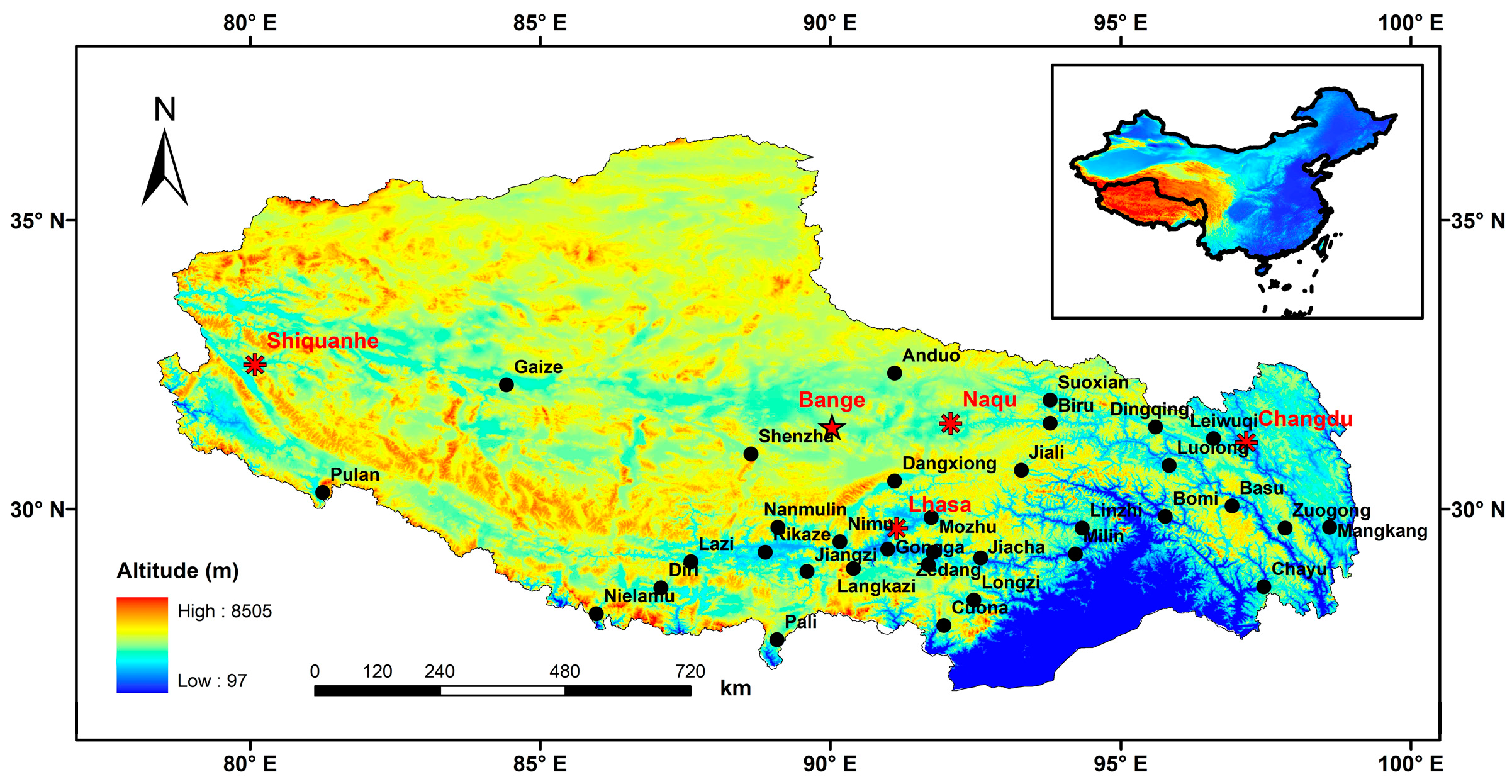
2.1. Data Collected in the Radiation Stations for Exploring the Effect of Calibration Data Length on the Performance of the Ångström–Prescott Model

Detailed information on radiation stations in the Tibetan Plateau is shown in

Table 1. Detailed information on radiation stations in Tibetan Plateau.

Station	Latitude/N	Longitude/E	Altitude/m
Lhasa	29.667	91.133	3648.9
Naqu	31.483	92.067	4507.0
Changdu	31.150	97.167	3306.0
Shiquanhe	32.500	80.083	4278.6

. All these 4 radiation stations in the Tibetan Plateau began routine observation in the 1950s or 1960s. However, owing to the inconsistency of data quality caused by instrument replacements, only the daily data observed from 1994 to 2017 were used in our study. For each of these radiation stations, the data from 1994 to 2013 were used for model calibration, while those from 2014 to 2017 were used for model validation.

Datasets with different lengths were generated to test the effects of calibration data length on the model performance. The dataset with length N was defined as the dataset that was composed of all the daily data in these N different years, and these years were selected randomly from 1994 to 2013. Thus, according to the combinatorial theory, the number of the datasets with length N should be C (20, N), based on which the same number of coefficients can be obtained by model calibration, respectively. For example, datasets with length 2 were those composed of data in 1994 and 1995, or the data in 1994 and 1996, or the data in 2012 and 2013, etc. The number of datasets with length 2 is C (20, 2), corresponding to the value of 190. Based on these 190 datasets, 190 sets of coefficients were obtained by model calibration, respectively. It should be noted that the total samples (n) for a dataset with length N, i.e., the number of the daily observations in different N years, is about N × 365 (366 in a leap year), instead of N. When N equals 20, the number of datasets with length 20 is C (20, 20), corresponding to the value of 1. In this situation, only one dataset was obtained, i.e., all data from 1994 to 2013 were used for calibration.

2.2. Data Measured during the Scientific Expedition for Model Calibration and Testing Different Paramerization Methods in the Central Tibetan Plateau

We used the daily observation data from 15 July 2014 to 22 September 2015 for model calibration and validation of the Ångström–Prescott model in Bange. All these daily observations were listed in sequence from 1 to 437. The daily observations with odd numbers were used for model calibration, while those with even numbers were used as the validation dataset.

In addition, assuming that no radiation observations were available in Bange, the coefficients in the Ångström–Prescott model could not be calibrated. Under this assumption, the coefficients were calculated directly from parametrization methods by the other meteorological or geographical factors such as latitude, altitude, and water vapor, etc. Based on the calculated coefficients, the daily radiation values were estimated by the Ångström–Prescott model, and the estimated values were further validated against the validation dataset.

2.3. Description of the Ångström–Prescott Model

The original Ångström–Prescott model was established by Ångström [16], and revised later by Prescott [17] as

$$\frac{Q}{Q_0}=a+b \frac{S}{S_0}$$

(1)

where Q is the solar radiation, Q₀ is the extraterrestrial radiation, S is the sunshine hours, and S₀ is the day length (potential sunshine hours), a and b are the coefficients of the Ångström–Prescott model. The sum of a and b represents the maximum clear sky atmospheric transmittance. This is the highest level of atmospheric transmittance that can occur when the sky is clear and free from abstractions (S = S₀). It is the maximum fraction of sunlight that can pass through the atmosphere and reach the Earth’s surface. The value a represents the minimum atmospheric transmittance when there is no sunshine (S = 0). This value corresponds to the situation when the sky is heavily overcast or cloudy, and very little sunlight is able to pass through the atmosphere. When both solar radiation and sunshine hours are observed, the coefficients of a and b in the Ångström–Prescott model can be calibrated with the corresponding observations.

However, when solar radiation observations are not available, the coefficients of a and b in the Ångström–Prescott model cannot be obtained by model calibration, which will limit the application of the Ångström–Prescott model. In this situation, the coefficients of a and b can be simply approximated by parameterization methods.

Based on the measured meteorological items and the relevant geographical factors in Bange, four different parameterization methods for calculating the coefficients in Bange are listed as follows.

(1)

FAO method

$$\frac{Q}{Q_0}=0.250+0.500\frac{S}{S_0}$$

(2)

where 0.250 and 0.500 are the coefficients of a and b, respectively, as recommended by FAO56 [34].

(2)

Gopinathan method

$$\frac{Q}{Q_0}=0.012+0.854\frac{S}{S_0}$$

(3)

where 0.012 and 0.854 are the coefficients of a and b in Bange, respectively. The coefficients were calculated based on the parameterization method by Gopinathan [38], with input variables such as the latitude, the altitude, and the long-term sunshine fractions in Bange.

$$a=-0.309+0.539\times cos\varphi -0.0693\times \lambda +0.290\times \overline{S/S_0}$$

(4)

$$b=1.527-1.027\times cos\varphi +0.0926\times \lambda -0.359\times \overline{S/S_0}$$

(5)

where $\varphi$ is the latitude, λ is the altitude, and $\overline{S/S_0}$ is the long-term annual average daily sunshine fraction in the Bange, respectively.

(3)

LiuXY method

$$\frac{Q}{Q_0}=0.244+0.636\frac{S}{S_0}$$

(6)

where 0.244 and 0.636 are the coefficients of a and b in Bange, respectively, which were calculated from the parameterization formulas as follows [5], with the input variable of the altitude in Bange.

$$(a+b)=0.0358\times \lambda +0.7121$$

(7)

$$a=0.0157\times \lambda +0.1705$$

(8)

(4)

LiuJD method

$$\frac{Q}{Q_0}=0.238+0.598\frac{S}{S_0}$$

(9)

The coefficients above were used for Bange, which were calculated from the following parameterization formulas [33], with the altitude and the water vapor pressure measured in Bange.

$$\left(a+b\right)=0.106\times \ln \left(\lambda \right)-0.060$$

(10)

$$b=0.373\times \frac{1}{\mu }+0.483$$

(11)

where µ is the average daily water vapor pressure (hPa) measured in Bange.

2.4. Model Evaluation

The statistics of the Nash–Sutcliffe efficiency (NSE), the root mean square error (RMSE), the mean absolute bias error (MABE), and the correlation coefficient (r) were used as indicators for evaluating model performance as follows [40,41,42,43].

$$NSE=1-\frac{{\sum }_{i=1}^n{(O_i-S_i)}^2}{{\sum }_{i=1}^n{(O_i-\overline{O})}^2}$$

(12)

$$RMSE=\sqrt{\frac{1}{n}{\sum }_{i=1}^n{(O_i-S_i)}^2}$$

(13)

$$MABE=\frac{1}{n}{\sum }_{i=1}^n\left|O_i-S_i\right|$$

(14)

$$r=\frac{{\sum }_{i=1}^n(O_i-\overline{O})(S_i-\overline{S})}{{\left({\sum }_{i=1}^n{(O_i-\overline{O})}^2{\sum }_{i=1}^n{(S_i-\overline{S})}^2\right)}^{0.5}}$$

(15)

where $O_i$ is the observed value, $S_i$ is the simulated value, $\overline{O}$ is the average value of the observed radiation, $\overline{S}$ is the average value of the simulated radiation, and n is the number of observations, respectively.

In addition, linear regressions were conducted between observed and simulated values, and slopes and interceptions of the regression lines were expressed as Slope and Inter, respectively, as auxiliary indicators to identify the overall discrepancy of the model simulations.

3. Results

First, we used various datasets observed in four radiation stations with different lengths to investigate the effects of calibration data length on the performance of the Ångström–Prescott model over the Tibetan Plateau, in order to test the reliability of calibration with short-term observations over the Tibetan Plateau. Then, scientific expedition observation data in Bange were analyzed and used for model calibration and evaluation of different parameterization methods in the central Tibetan Plateau.

3.1. Exploration of the Effect of Calibration Length on the Performance of the Ångström–Prescott Model over the Tibetan Plateau

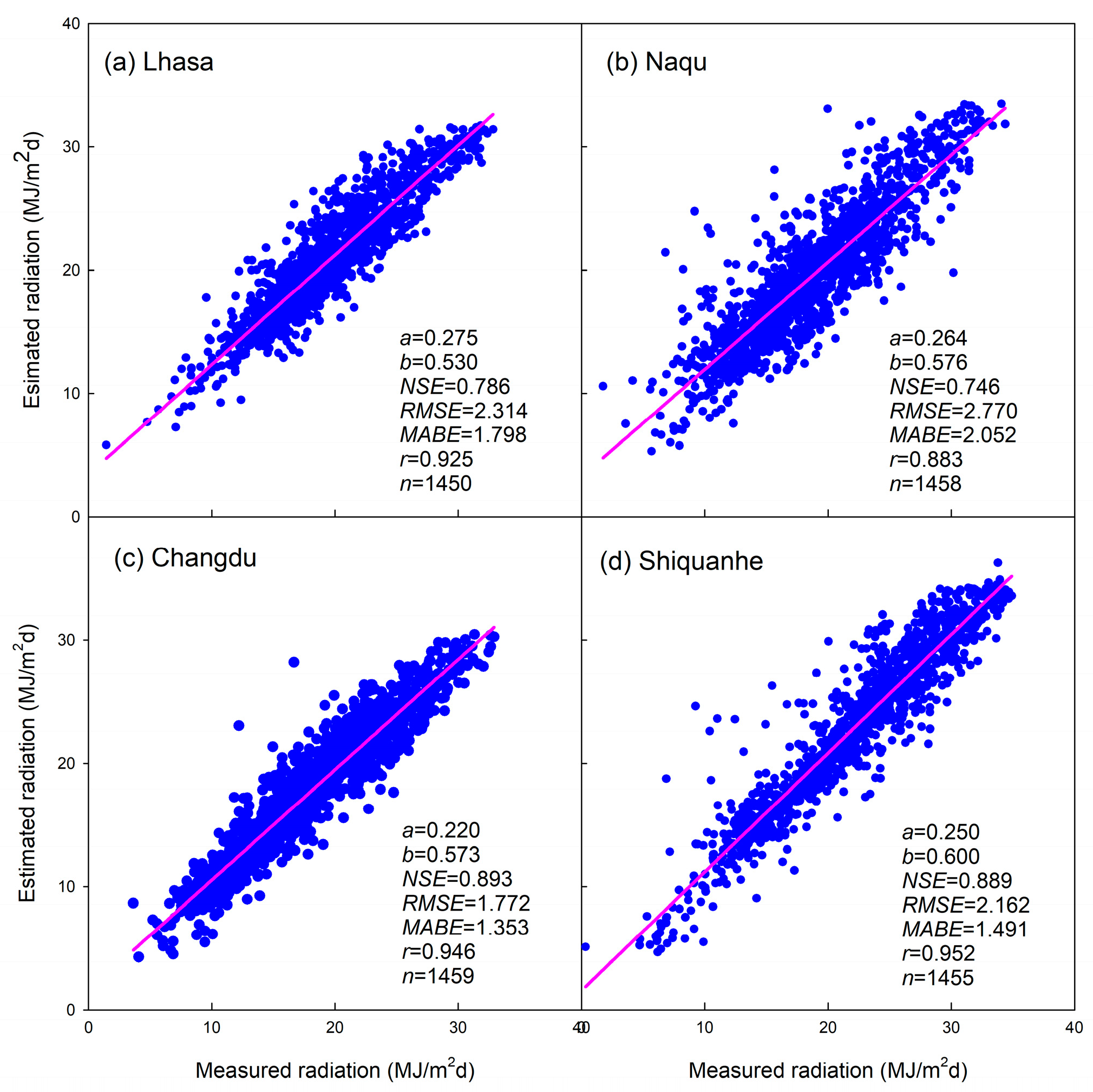
3.1.1. Calibration of the Ångström–Prescott Model in Routine Method

Routinely, all the radiation data were divided into two datasets, one for calibration and the other for validation. According to this routine operation, all data in 1994–2013 were used for calibration, and the data in 2014–2017 were used for model validation.

It can be seen that both of the coefficients obviously changed among different stations (Figure 2). The values of the coefficient a ranged from 0.220 in Changdu to 0.275 in Lhasa, with an average value of 0.252. In contrast to the smaller values of coefficient a, all values of the coefficient b were above 0.500, ranging from 0.530 in Lhasa to 0.600 in Shiquanhe, with an average value of 0.570 (Figure 2).

The validation results showed that the calibrated Ångström–Prescott model performed well, with high values of NSE and low values of RMSE in all these four radiation stations (Figure 2). The value of NSE changed from 0.746 in Naqu to 0.893 in Changdu with an average value as high as 0.828. Additionally, comparison between the regression line and the diagonal line for each station confirmed that the Ångström–Prescott model could estimate accurately the solar radiation over ATR, when the calibration was conducted with local observations.

The lowest value of b occurred in Lahsa (Figure 2). Lhasa is the largest city in the Tibetan Plateau, which might be the source of more anthropogenic pollution than the surrounding cities on the Tibetan Plateau. The relevant anthropogenic pollution sources can somewhat influence sky conditions, and further result in the lowest value of b in Lhasa. The value of b in Changdu was 0.573, lower than that in Naqu and Shiquanhe. The altitudes in Changdu, Naqu, and Shiquanhe were 3306.0 m, 4507.0 m, and 4278.6 m, respectively. This implies that the altitude might play an important role in the value of b. Further comparison of the values of b in Naqu and Shiquanhe indicates that Shiquanhe had a larger value of b than Naqu (Figure 2), though the altitude in Naqu is higher than that in Shiquanhe. Thus, besides altitude, other factors such as water vapor, etc., also play important roles in the value of b [7].

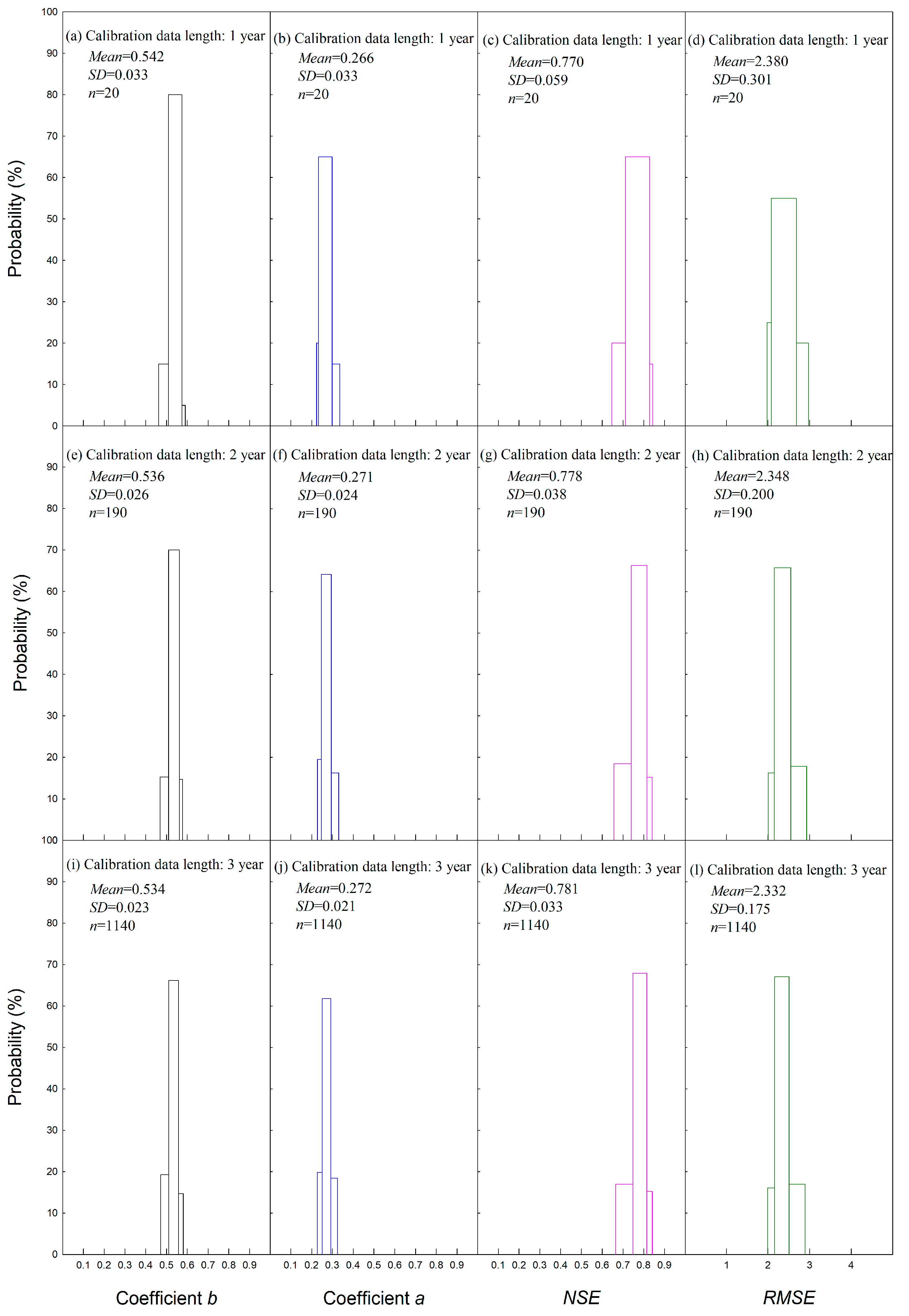
3.1.2. Calibration of the Ångström–Prescott Model with Different Data Lengths

When calibration data length was set as 1, i.e., only 1 year was randomly selected from 1994–2013, there were 20 different datasets for calibration, and each dataset had a sample of 365 (or 366) daily observations. So, 20 sets of the coefficients of a and b were obtained by model calibration (

Table 2. Validation results of the Ångström–Prescott model with the coefficients calibrated by different data lengths.

Station	DL	b	a	NSE	RMSE	MABE	r	DN	n
Lhasa	1	0.542 ± 0.033	0.266 ± 0.033	0.770 ± 0.059	2.380 ± 0.301	1.872 ± 0.265	0.923 ± 0.002	20	365–366
	2	0.536 ± 0.026	0.271 ± 0.024	0.778 ± 0.038	2.348 ± 0.200	1.835 ± 0.175	0.924 ± 0.002	190	730–732
	3	0.534 ± 0.023	0.272 ± 0.021	0.781 ± 0.033	2.332 ± 0.175	1.819 ± 0.153	0.924 ± 0.002	1140	1095–1098
Naqu	1	0.573 ± 0.031	0.266 ± 0.022	0.718 ± 0.055	2.905 ± 0.276	2.187 ± 0.248	0.882 ± 0.004	20	365–366
	2	0.573 ± 0.020	0.266 ± 0.015	0.732 ± 0.041	2.837 ± 0.210	2.119 ± 0.188	0.882 ± 0.003	190	730–732
	3	0.571 ± 0.016	0.267 ± 0.012	0.737 ± 0.032	2.814 ± 0.169	2.095 ± 0.151	0.882 ± 0.002	1140	1095–1098
Changdu	1	0.570 ± 0.053	0.221 ± 0.023	0.862 ± 0.050	1.989 ± 0.318	1.544 ± 0.293	0.945 ± 0.002	20	365–366
	2	0.571 ± 0.036	0.222 ± 0.016	0.877 ± 0.021	1.893 ± 0.150	1.453 ± 0.134	0.946 ± 0.001	190	730–732
	3	0.569 ± 0.029	0.222 ± 0.013	0.884 ± 0.011	1.843 ± 0.088	1.411 ± 0.081	0.946 ± 0.001	1140	1095–1098
Shiquanhe	1	0.587 ± 0.106	0.260 ± 0.080	0.838 ± 0.125	2.499 ± 0.766	1.840 ± 0.768	0.948 ± 0.011	20	365–366
	2	0.584 ± 0.085	0.260 ± 0.066	0.868 ± 0.052	2.320 ± 0.400	1.661 ± 0.399	0.950 ± 0.006	190	730–732
	3	0.572 ± 0.083	0.273 ± 0.066	0.869 ± 0.044	2.320 ± 0.356	1.653 ± 0.353	0.950 ± 0.004	1140	1095–1098

Note: DL, DN, and n denote data length, dataset number, and samples in each dataset, respectively. In the expression of M ± S, M denotes mean value, and S standard deviation, respectively. When data lengths of 1, 2, and 3 years were selected from the dataset from 1994 to 2013, the number of calibration datasets were 20 (C(20, 1)), 190 (C(20, 2)), and 1140 (C(20, 3)), respectively, and the corresponding data numbers (n) in each dataset for calibration were 365–366, 730–732, and 1095–1098, respectively.

). Statistical analysis of these 20 sets of coefficients indicated that their values were quite stable, with a small standard deviation. It is notable that the mean values of the coefficient b in Lhasa, Naqu, Changdu, and Shiquanhe were 0.542, 0.573, 0.570, and 0.587 (Table 2), which were very close to the corresponding values of 0.530, 0.576, 0.573, and 0.600 calibrated with 20-year data length (Figure 2), respectively. Therefore, we concluded that the coefficients calibrated with 1-year observations were comparable to those with 20-year observations. The statistical analysis of the coefficient a showed a very similar result (Table 2).

Then, we used each of these 20 sets of calibrated coefficients to run the Ångström–Prescott model for validation against the data in 2014–2017, and we obtained 20 sets of NSE, RMSE, MABE and r accordingly. Just as the variations in the coefficients of a and b, these 20 sets of NSE, RMSE, MABE, and r were also quite stable with small standard deviations (Table 2). Most importantly, high values of NSE occurred in all stations (Table 2), indicating that the Ångström–Prescott model performed well in all these four stations even with 1-year data for calibration. In addition, it should be noted that the mean values of NSE in Lhasa, Naqu, Changdu, and Shiquanhe were 0.770, 0.718, 0.862, and 0.838, respectively (Table 2). In contrast, with 20-year data for calibration, the corresponding values of NSE were 0.786, 0.746, 0.893, and 0.889, respectively (Figure 2). So, the values of NSE with 1-year data for calibration were quite comparable to those with 20-year observations, so the calibration with a long-term dataset had little advantage over that with short-term observations.

When the data length increased to 2 and 3, both the calibrated coefficients (a and b) and the performance indicators (NSE, RMSE, MABE, and r) showed little change, and the values of the coefficients and the indicators showed statistical characteristics very similar to those with data length of 1 (Table 2). When the calibration data length was larger than 3, the calibration and validation results were nearly unchanged and not shown due to limitations of the space. For a clear illustration, the probability distribution of the coefficients and indicators in Lhasa are shown in Figure 3, using the same statistical data in Table 2. This table shows vividly that all of these parameters were quite stable, and the statistical characteristics were nearly unchanged with calibration data length increasing (Figure 3).

3.2. Model Calibration and Evaluation of Different Parametrization Methods with Expedition Observations in Bange

3.2.1. Preliminary Analysis of the Expedition Data in Bange

The solar radiation at noon varied significantly from 72.6 J/m²s on a cloudy day to 1216.6 J/m²s on a clear day (Figure 4a). On the clear days, the ratio of observed radiation to extraterrestrial radiation was as high as 0.95. The extreme case occurred on 15 January 2015, when the observed radiation was even higher than the extraterrestrial radiation. It is common knowledge that the surface solar radiation should never be higher than the extraterrestrial radiation, but this kind of extreme phenomenon does exist over the Tibetan Plateau and will be discussed later in detail.

The daily solar radiation changed from 8.6 MJ/m²d on a cloudy day to 34.6 MJ/m²d on a clear day (Figure 4b). The monthly averaged daily solar radiation ranged from 15.2 MJ/m²d in December 2014 to 26.5 MJ/m²d in July 2015, with an average value of 20.64 MJ/m²d from July 2014 to August 2015.

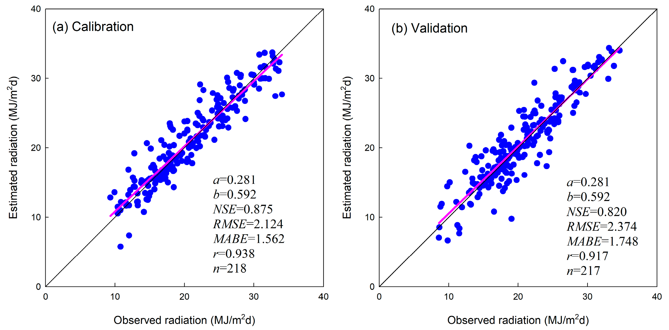
3.2.2. Calibration of the Ångström–Prescott Model with Observations in Bange

As described in the Data and Method section, 218 expedition data with odd numbers in the sequence were used to calibrate the Ångström–Prescott model in Bange. The coefficients of a and b in Bange were 0.281 and 0.592, respectively (Figure 5a). Then, the calibrated Ångström–Prescott model was validated against 217 expedition data with even numbers in the sequence (Figure 5b). High values of NSE and low values of RMSE in both calibration and validation processes indicated that the Ångström–Prescott model performed well in Bange with the support of the expedition data (Figure 5). The value of NSE was 0.820 in the validation process, a little less than the 0.875 in the calibration process. This can be viewed as a normal phenomenon according to the relevant statistical theory [41].

3.2.3. Evaluation of Different Parametrization Methods for Calculating the Coefficients of the Ångström–Prescott Model in Bange

If no radiation data were available for model calibration, the coefficients of a and b would have to be estimated by some parametrization methods. According to Equations (2), (3), (6) and (9), all of these four parameterization methods, including the FAO method, Gopinathan method, LiuXY method, and LiuJD method, were validated against the 217 daily validation data in Bange, and the corresponding results are shown in Figure 6.

When the Ångström–Prescott model was validated with the coefficients estimated by the parameterization methods, all the values of NSE were much lower than the value of 0.820 above in the validation with the coefficients calibrated by local observations. The Gopinathan method performed worst, with the lowest NSE of 0.218 and the highest RMSE of 4.948, respectively (Figure 6b). In addition, the coefficients estimated by this method were not comparable to those obtained by the other methods, with a much lower value of coefficient a and very much higher value of coefficient b. The FAO method performed better than the Gopinathan method, due to its comparable coefficients of a and b, together with its higher NSE of 0.578 (Figure 6a). However, the FAO method was significantly outperformed by both the LiuXY method and the LiuJD method (Figure 6c,d). The LiuXY method resulted in a better performance with a higher NSE of 0.764. Additionally, its slope of linear regression was very close to 1, and its interception was very close to 0, so the simulated radiation agreed well with the observations as a whole (Figure 6c). The LiuJD method showed a model performance very similar to that of the LiuXY method, but the NSE of the LiuJD method was 0.792, a little higher than that of the LiuXY method, indicating that the LiuJD method performed best among these four parameterization methods.

4. Discussion

4.1. Characteristics of the Coefficients of a and b over the Tibetan Plateau

All the coefficients of b over the Tibetan Plateau, whether calibrated with short-term observations measured in scientific expeditions or long-term data collected at radiation stations, were within the range of 0.530 to 0.600 (Figure 2 and Figure 5). They were higher than the value of 0.500 recommended by the FAO [34], which can be explained by the roles that the coefficients play in the Ångström–Prescott model. According to the relevant theory, the coefficient a is the solar radiation reaching the surface of the earth on a cloudy day [44], which is mainly affected by the local cloud conditions [45]. In contrast, the coefficient b can be viewed as a kind of transmissivity of solar radiation under cloudless conditions [5], which is mainly influenced by atmospheric conditions such as air mass, water vapor content, and aerosol density [46]. The relatively lower aerosol density due to the clean conditions [37], together with the small air mass caused by the high elevation over the Tibetan Plateau, resulted in the high transmissivities of the larger values of coefficient b at these locations (Figure 2 and Figure 5).

The coefficients of a and b changed obviously among different locations (Figure 2), but remained relatively stable locally at each station (Table 2 and Figure 3). This characteristic was consistent with those identified in the other regions [5,30], and can also be explained by the same theory above. The Tibetan Plateau is one of the areas with the most complex terrains in the world [47], and its climate conditions, including cloud conditions, vary obviously among different locations due to its complex topographic elevations [48]. This kind of spatial variation in both cloud conditions and regional altitudes make the coefficients of a and b vary significantly among different locations. However, for a certain site, the cloud condition is relatively stable, and the water vapor content has little inter-annual variation [49]. More importantly, the air mass remains unchanged due to the fixed altitude of a certain site. Thus, all these factors discussed above make the coefficients of a and b quite stable locally. Further, the locally stable coefficients make the calibration reliable even with short-term expedition observations over the Tibetan Plateau.

4.2. Unrealistic Global Parameterization Method and Necessary Local Calibration over the Tibetan Plateau

As the radiation stations are distributed sparsely, calibration of the Ångström–Prescott model is difficult in most regions. Under this condition, some scientists tried to suggest some general parameterization methods to make the coefficients readily available [5,33,34,38,50]. The simplest parameterization method is recommended by the FAO with the coefficients of a and b directly set as the fixed values of 0.250 and 0.500, respectively [34]. However, these suggested coefficients are not comparable to the calibrated ones in many locations in China [30], and they are quite different from those calibrated over the Tibetan Plateau (Figure 1 and Figure 5), which inevitably resulted in the poor model performance, as shown in Figure 6a. In contrast to the simple fixed coefficients suggested by the FAO, the Gopinathan parameterization method was based on the coefficients calibrated at 40 stations around the world and validated against observations at 14 stations located across a wide range [38]. The stations involved in the model establishment covered a wide range of geographical and climate conditions, hence Gopinathan et al. [38] believed the method was capable of worldwide application. However, it was found later that the Gopinathan method performed poorly in Turkey [51]. Even more, the Gopinathan method performed the worst among all selected methods for estimating solar radiation in China [5]. In addition, with the lowest NSE of 0.218 and the highest RMSE of 4.948, the Gopinathan method showed the worst performance among the four selected parameterization methods tested in this study (Figure 6), which was quite consistent with both of the previous reports [5,51]. Based on these findings, we anticipate that global parameterization methods, aiming to provide coefficients worldwide for model application, might be unrealistic and should be used with caution in local radiation estimations.

In contrast, the parameterization methods can perform much better if they are based on the coefficients calibrated locally. The LiuXY method was established with the coefficients calibrated at 34 stations in China [52] and believed to be the best parameterization method among all selected models by a later validation at 80 stations over China [5]. With a high NSE of 0.764 and a low RMSE of 2.718 (Figure 6c), its validation results can be viewed as acceptable in case no data are available for calibration of the Ångström–Prescott model in the Tibetan Plateau. Compared with the LiuXY method, the LiuJD method performed even better with the highest NSE of 0.792 and the lowest RMSE of 2.551, respectively (Figure 6d). The best model performance of the LiuJD method can be attributed to the coefficients used for parameterization, which were calibrated with the observations at 15 radiation stations over the Tibetan Plateau [33]. Thus, the findings in this study further emphasize the importance of local calibration of the Ångström–Prescott model, especially in regions with complex terrain conditions such as the Tibetan Plateau. We propose that the most reliable strategy for determining coefficients of the Ångström–Prescott model is to make calibration locally with observations from radiation stations or from short-term scientific expeditions. If no data are available for local calibration, the coefficients of the Ångström–Prescott model should be estimated by parameterization methods based on calibration at the surrounding stations, the nearer the better.

4.3. Uncertainties and Future Research

Because of its unique climate conditions [48], the Tibetan Plateau occasionally exhibits some extreme weather phenomena quite different from those observed elsewhere, at lower altitudes. In this study, the extremely high radiation occurred at noon on 15 January 2015, with a value even higher than the corresponding extraterrestrial radiation (Figure 4a). This can be viewed as an impossible phenomenon according to the relevant radiation theory [53], as the surface solar radiation comes from the extraterrestrial radiation through various factors such as air mass, water vapor content, clouds, and aerosol particles [53]. Therefore, the surface solar radiation should be less than the extraterrestrial radiation accordingly. However, this kind of abnormal phenomenon was noted in the scientific expeditions over the Tibetan Plateau as early as the 1980s, and about 60 instances of this kind of abnormal phenomenon were observed in Lhasa over the Tibetan Plateau in the summer of 1995 [54]. Currently, this kind of extreme phenomenon is commonly accepted by Tibetan climatologists in China, but a huge amount of uncertainty still exists concerning aspects such as the reason for and the pattern of its occurrence. Thus, these uncertainties and the relevant underlying mechanisms should be further investigated, as they could become a very troublesome issue in the estimation of solar radiation on hourly scales [55,56].

5. Conclusions

The coefficients of the Ångström–Prescott model changed obviously among different stations over the Tibetan Plateau due to its unique climate condition and complex terrains. However, the coefficients were kept relatively stable at each station owing to local stable cloud conditions, the unchanged air mass, and the little inter-annual variations in water vapor content. Thus, calibration with 1-year observations resulted in model performances comparable to those with 20-year calibration data, and we predict that calibration with short-term scientific expedition observations is reliable over the Tibetan Plateau.

Analysis of the 435 daily observations measured in a scientific expedition showed that the monthly average daily solar radiation ranged from 15.2 MJ/m²d in December 2014 to 26.5 MJ/m²d in July 2015, with an average value of 20.64 MJ/m²d. Calibrated with the expedition data, the Ångström–Prescott model performed well with an NSE of 0.820. In contrast, the Ångström–Prescott model performed worse when the coefficients were estimated by parameterization methods. Among four selected parameterization methods, the LiuJD method performed best with an NSE of 0.792, followed by the LiuXY method with a close NSE of 0.764. The FAO method is recommended for worldwide application with fixed coefficients but performed worse with an NSE of 0.620. Additionally, the Gopinathan method, which was established based on the radiation data collected over a wide range in the world, performed the worst with the lowest NSE of 0.218.

Drawing from these insights, we recommend the following strategies for solar radiation estimation over the Tibetan Plateau. The most dependable approach involves using the Ångström–Prescott model calibrated with observation data, even if gathered from short-term scientific expeditions. When calibration data are unavailable, coefficients of the Ångström–Prescott model should be approximated through parameterization methods based on neighboring radiation stations’ calibrations. We caution that general parameterization methods designed for global application are not suitable for determining coefficients to estimate solar radiation over the Tibetan Plateau due to their unreliability and subsequent poor model performance in this region.

References

1. Gueymard, C.A. The sun’s total and spectral irradiance for solar energy applications and solar radiation models. Sol. Energy 2004, 76, 423–453. [Google Scholar] [CrossRef]
2. Ordoñez Palacios, L.E.; Bucheli Guerrero, V.; Ordoñez, H. Machine learning for solar resource assessment using satellite images. Energies 2022, 15, 3985. [Google Scholar] [CrossRef]
3. Hunt, L.A.; Kuchar, L.; Swanton, C.J. Estimation of solar radiation for use in crop modeling. Agric. For. Meteorol. 1998, 91, 293–300. [Google Scholar] [CrossRef]
4. Miller, D.G.; Rivington, M.; Matthews, K.B.; Bellocchi, G. Testing the spatial applicability of the Johnson-Woodward method for estimating solar radiation from sunshine duration data. Agric. For. Meteorol. 2008, 148, 466–480. [Google Scholar] [CrossRef]
5. Liu, X.; Xu, Y.; Zhong, X.; Zhang, W.; Porter, J.R.; Liu, W.L. Assessing models for parameters of the Ångström-Prescott formula in China. Appl. Energy 2012, 96, 327–338. [Google Scholar] [CrossRef]
6. Li, H.; Ma, W.; Lian, Y.; Wang, X.; Zhao, L. Global solar radiation estimation with sunshine duration in Tibet, China. Renew. Energy 2011, 36, 3141–3145. [Google Scholar] [CrossRef]
7. Liu, J.; Liu, J.; Linderholm, H.W.; Chen, D.; Yu, Q.; Wu, D.; Haginoya, S. Observation and calculation of the solar radiation on the Tibetan Plateau. Energy Convers. Manag. 2012, 57, 23–32. [Google Scholar] [CrossRef]
8. Wolf, K.; Ehrlich, A.; Mech, M.; Hogan, R.; Wendisch, M. Evaluation of ECMWF radiation scheme using aircraft observations of spectral irradiance above clouds. J. Atmos. Sci. 2020, 77, 2665–2685. [Google Scholar] [CrossRef]
9. Varga, A.J.; Breuer, H. Sensitivity of simulated temperature, precipitation, and global radiation to different WRF configurations over the Carpathian Basin for regional climate applications. Clim. Dyn. 2020, 55, 2849–2866. [Google Scholar] [CrossRef]
10. Wong, M.S.; Zhu, R.; Liu, Z.; Lu, L.; Peng, J.; Tang, Z.; Chan, W.K. Estimation of Hong Kong’s solar energy potential using GIS and remote sensing technologies. Renew. Energy 2016, 99, 325–335. [Google Scholar] [CrossRef]
11. Song, X.; Huang, Y.; Zhao, C.; Liu, Y.; Lu, Y.; Chang, Y.; Yang, J. An approach for estimating solar photovoltaic potential based on rooftop retrieval from remote sensing images. Energies 2018, 11, 3172. [Google Scholar] [CrossRef]
12. Pinker, R.T.; Frouin, R.; Li, Z. A review of satellite methods to derive surface shortwave irradiance. Remote Sens. Environ. 1995, 51, 108–124. [Google Scholar] [CrossRef]
13. Voyant, C.; Notton, G.; Kalogirou, S.; Nivet, M.L.; Paoli, C.; Motte, F.; Fouilloy, A. Machine learning methods for solar radiation forecasting: A review. Renew. Energy 2017, 105, 569–582. [Google Scholar] [CrossRef]
14. Taki, M.; Rohani, A.; Yildizhan, H. Application of machine learning for solar radiation modeling. Theor. Appl. Climatol. 2021, 143, 1599–1613. [Google Scholar] [CrossRef]
15. Zhou, L.; Pan, S.; Wang, J.; Vasilakos, A.V. Machine learning on big data: Opportunities and challenges. Neurocomputing 2017, 237, 350–361. [Google Scholar] [CrossRef]
16. Ångström, A. Solar and terrestrial radiation. Q. J. R. Met. Soc. 1924, 50, 121–125. [Google Scholar] [CrossRef]
17. Prescott, J.A. Evaporation from a water surface in relation to solar radiation. Trans. R. Soc. S. Aust. 1940, 64, 114–118. [Google Scholar]
18. Bristow, K.L.; Campbell, G.S. On the relationship between incoming solar radiation and daily maximum and minimum temperature. Agric. For. Meteorol. 1984, 31, 159–166. [Google Scholar] [CrossRef]
19. Hargreaves, G.L.; Hargreaves, G.H.; Riley, J.P. Irrigation water requirements for Senegal River Basin. J. Irrig. Drain. Eng. 1985, 111, 265–275. [Google Scholar] [CrossRef]
20. Meza, F.; Varas, E. Estimation of mean monthly solar global radiation as a function of temperature. Agric. For. Meteorol. 2000, 100, 231–241. [Google Scholar] [CrossRef]
21. McCaskill, M.R. Prediction of solar radiation from rain day information using regionally stable coefficients. Agric. For. Meteorol. 1990, 51, 247–255. [Google Scholar] [CrossRef]
22. Hook, J.E.; McClendon, R.W. Estimation of solar radiation data missing from long-term meteorological records. Agron. J. 1992, 84, 739–742. [Google Scholar] [CrossRef]
23. Wu, G.; Liu, Y.; Wang, T. Methods and strategy for modeling daily global solar radiation with measured meteorological data—A case study in Nanchang station, China. Energy Convers. Manag. 2007, 48, 2447–2452. [Google Scholar] [CrossRef]
24. Gouda, S.G.; Hussein, Z.; Luo, S.; Yuan, Q. Review of empirical solar radiation models for estimating global solar radiation of various climate zones of China. Prog. Phys. Geogr. Earth Environ. 2020, 44, 168–188. [Google Scholar] [CrossRef]
25. Ogolo, E.O. Evaluating the performance of some predictive models for estimating global solar radiation across the varying climatic conditions in Nigeria. Pac. J. Sci. Technol. 2010, 11, 60–72. [Google Scholar]
26. Adaramola, M.S. Estimating global solar radiation using common meteorological data in Akure, Nigeria. Renew. Energy 2012, 47, 38–44. [Google Scholar] [CrossRef]
27. Thornton, P.E.; Running, S.W. An improved algorithm for estimating incident daily solar radiation from measurements of temperature, humidity, and precipitation. Agric. For. Meteorol. 1999, 93, 211–228. [Google Scholar] [CrossRef]
28. Weiss, A.; Hays, C.J. Simulation of daily solar irradiance. Agric. For. Meteorol. 2004, 123, 187–199. [Google Scholar] [CrossRef]
29. Liu, D.L.; Scott, B.J. Estimation of solar radiation in Australia from rainfall and temperature observation. Agric. For. Meteorol. 2001, 106, 41–59. [Google Scholar] [CrossRef]
30. Chen, R.; Kang, E.; Yang, J.; Lu, S.; Zhao, W. Validation of five global radiation models with measured daily data in China. Energy Convers. Manag. 2004, 45, 1759–1769. [Google Scholar] [CrossRef]
31. Chen, R.; Kang, E.; Lu, S.; Yang, J.; Ji, X.; Zhang, Z.; Zhang, J. New methods to estimate global radiation based on meteorological data in China. Energy Convers. Manag. 2006, 47, 2991–2998. [Google Scholar] [CrossRef]
32. Liu, X.; Mei, X.; Li, Y.; Wang, Q.; Jensen, J.R.; Zhang, Y.; Porter, J.R. Evaluation of temperature-based global solar radiation models in China. Agric. For. Meteorol. 2009, 149, 1433–1446. [Google Scholar] [CrossRef]
33. Liu, J.; Pan, T.; Chen, D.; Zhou, X.; Yu, Q.; Flerchinger, G.N.; Shen, Y. An improved Ångström-type model for estimating solar radiation over the Tibetan Plateau. Energies 2017, 10, 892. [Google Scholar] [CrossRef]
34. Allen, R.G.; Pereira, L.S.; Raes, D.; Smith, M. Crop Evapotranspiration—Guidelines for Computing Crop Water Requirements; FAO Irrigation and Drainage Paper 56; Food and Agriculture Organization of the United Nations: Rome, Italy, 1998; Volume 300, p. D05109. [Google Scholar]
35. Liu, J.; Linderholm, H.; Chen, D.; Zhou, X.; Flerchinger, G.N.; Yu, Q.; Yang, Z. Changes in the relationship between solar radiation and sunshine duration in large cities of China. Energy 2015, 82, 589–600. [Google Scholar] [CrossRef]
36. Pelkowski, J. A physical rationale for generalized Ångström–Prescott regression. Sol. Energy 2009, 83, 955–963. [Google Scholar] [CrossRef]
37. Streets, D.G.; Yu, C.; Wu, Y.; Chin, M.; Zhao, Z.; Hayasaka, T.; Shi, G. Aerosol trends over China, 1980–2000. Atmos. Res. 2008, 88, 174–182. [Google Scholar] [CrossRef]
38. Gopinathan, K.K. A general formula for computing the coefficients of the correlation connecting global solar radiation to sunshine duration. Sol. Energy 1988, 41, 499–502. [Google Scholar] [CrossRef]
39. Jiang, Y.; Shi, B.; Su, G.; Lu, Y.; Li, Q.; Meng, J.; Ding, Y.; Song, S.; Dai, L. Spatiotemporal analysis of ecological vulnerability in the Tibet Autonomous Region based on a pressure-state-response-management framework. Ecol. Indic. 2021, 130, 108054. [Google Scholar] [CrossRef]
40. Nash, J.E.; Sutcliffe, J.V. River flow forecasting through conceptual models. I. A discussion of principles. J. Hydrol. 1970, 10, 282–290. [Google Scholar] [CrossRef]
41. Von Storch, H.; Zwiers, F.W. Statistical Analysis in Climate Research; Cambridge University Press: Cambridge, UK, 2001; pp. 3–10. [Google Scholar]
42. Gouda, S.G.; Hussein, Z.; Luo, S.; Wang, P.; Gao, H.; Yuan, Q. Empirical models for estimating global solar radiation in Wuhan City, China. Eur. Phys. J. Plus 2018, 133, 517. [Google Scholar] [CrossRef]
43. Gouda, S.G.; Hussein, Z.; Luo, S.; Yuan, Q. Model selection for accurate daily global solar radiation prediction in China. J. Clean. Prod. 2019, 221, 132–144. [Google Scholar] [CrossRef]
44. Almorox, J.; Hontoria, C. Global solar radiation estimation using sunshine duration in Spain. Energy Convers. Manag. 2004, 45, 1529–1535. [Google Scholar] [CrossRef]
45. De Souza, J.L.; Lyra, G.B.; Dos Santos, C.M.; Ferreira Junior, R.A.; Tiba, C.; Lyra, G.B.; Lemes, M.A.M. Empirical models of daily and monthly global solar irradiation using sunshine duration for Alagoas State, Northeastern Brazil. Sustain. Energy Technol. Assess. 2016, 14, 35–45. [Google Scholar] [CrossRef]
46. Yang, K.; Huang, G.W.; Tamai, N. A hybrid model for estimating global solar radiation. Sol. Energy 2001, 70, 13–22. [Google Scholar] [CrossRef]
47. Kattel, D.B.; Yao, T. Temperature-topographic elevation relationship for high mountain terrain: An example from the southeastern Tibetan Plateau. Int. J. Climatol. 2018, 38, 901–920. [Google Scholar] [CrossRef]
48. Domros, M.; Peng, G.B. The Climate of China; Springer: Berlin/Heidelberg, Germany, 1988. [Google Scholar]
49. Liu, J.; Sun, Z.; Liang, H. Precipitable water vapor on the Tibetan Plateau estimated by GPS, water vapor radiometer, radiosonde, and numerical weather prediction analysis and its impact on the radiation budget. J. Geophys. Res. 2005, 110, D17106. [Google Scholar] [CrossRef]
50. Liu, Y.; Tan, Q.; Pan, T. Determining the parameters of the Ångström-Prescott model for estimating solar radiation in different regions of China: Calibration and modeling. Earth Space Sci. 2019, 6, 1976–1986. [Google Scholar] [CrossRef]
51. Ertekin, C.; Evrendilek, F. Spatio-temporal modeling of global solar radiation dynamics as a function of sunshine duration for Turkey. Agric. For. Meteorol. 2007, 45, 36–47. [Google Scholar] [CrossRef]
52. Liu, X.; Mei, X.; Li, Y.; Wang, Q.; Zhang, Y.; Porter, J.R. Variation in reference crop evapotranspiration caused by the Ångström–Prescott coefficient: Locally calibrated versus the FAO recommended. Agric. Water Manag. 2009, 96, 1137–1145. [Google Scholar] [CrossRef]
53. Lutgens, F.K.; Tarbuk, E.J. The Atmosphere: An Introduction to Meteorology; Prentice Hall: Hoboken, NJ, USA, 2001. [Google Scholar]
54. Li, C.; Gong, Y.; Duan, T. Observational study of super solar constant of the solar radiation over Qinghai-Tibet Plateau. J. Chengdu Inst. Meteorol. 2000, 53, 107–112. [Google Scholar]
55. Chang, K.; Zhang, Q. Improvement of the hourly global solar model and solar radiation for air-conditioning design in China. Renew. Energy 2019, 138, 1232–1238. [Google Scholar] [CrossRef]
56. Li, D.H.; Chen, W.; Li, S.; Lou, S. Estimation of hourly global solar radiation using Multivariate Adaptive Regression Spline (MARS)—A case study of Hong Kong. Energy 2019, 186, 115857. [Google Scholar] [CrossRef]
Figure 1. Location of the experimental site and distribution of weather stations over the Tibetan Plateau. The red five-pointed star denotes the experimental site in Bange, and the red asterisks denote the radiation stations over the Tibetan Plateau. The black dots denote ordinary weather stations without radiation observations.
Energies 16 07093 g001
Figure 2. Validation of Ångström–Prescott model with coefficients calibrated by 20-year observations at four radiation stations: (a) Lhasa; (b) Naqu; (c) Changdu; and (d) Shiquanhe.
Energies 16 07093 g002
Figure 3. Probability distribution of the calibrated coefficients and model performance indicators in Lhasa under different data lengths: (ad) 1-year data length; (eh) 2-year data length; (il) 3-year data length.
Energies 16 07093 g003
Figure 4. Seasonal variation of the observed radiation in Bange. (a) Global radiation at noon time; (b) daily global radiation.
Energies 16 07093 g004
Figure 5. Calibration and validation of the Ångström–Prescott model in Bange: (a) calibration; (b) validation.
Energies 16 07093 g005
Figure 6. Model performance in Bange under different parameterization methods: (a) FAO method; (b) Gopinathan method; (c) LiuXY method; and (d) LiuJD method.
Energies 16 07093 g006