Abstract
The accuracy of pipeline temperature monitoring using the Brillouin Optical Time Domain Analysis system depends on the Brillouin Gain Spectrum in the Brillouin Optical Time Domain Analysis system. The Non-Local Means noise reduction algorithm, due to its ability to use the data patterns available within the two-dimensional measurement data space, has been used to improve the Brillouin Gain Spectrum in the Brillouin Optical Time Domain Analysis system. This paper studies a new Non-Local Means algorithm optimized through the Black Widow Optimization Algorithm, in view of the unreasonable selection of smoothing parameters in other Non-Local Means algorithms. The field test demonstrates that, the new algorithm, when compared to other Non-Local Means methods, excels in preserving the detailed information within the Brillouin Gain Spectrum. It successfully restores the fundamental shape and essential characteristics of the Brillouin Gain Spectrum. Notably, at the 25 km fiber end, it achieves a 3 dB higher Signal-to-Noise Ratio compared to other Non-Local Means noise reduction algorithms. Furthermore, the Brillouin Gain Spectrum values exhibit increases of 9.4% in Root Mean Square Error, 12.5% in Sum of Squares Error, and 10% in Full Width at Half Maximum. The improved method has a better denoising effect and broad application prospects in pipeline safety.
1. Introduction
1.1. Background
Pipelines play an important role in long-distance energy transportation. However, oil pipelines have the characteristics of long distances, mostly buried underground, and complex geological environments in their surrounding areas [1]. After long-term service, failure accidents will occur due to terrain settlement, corrosion, pipe and construction integrity, mechanical construction impairments, and other causes. Since pipelines operate under high pressure and the transport medium is flammable and explosive, once an accident occurs, it is easy to cause heavy losses. Therefore, it is very important to monitor the safety state of pipelines [2,3].
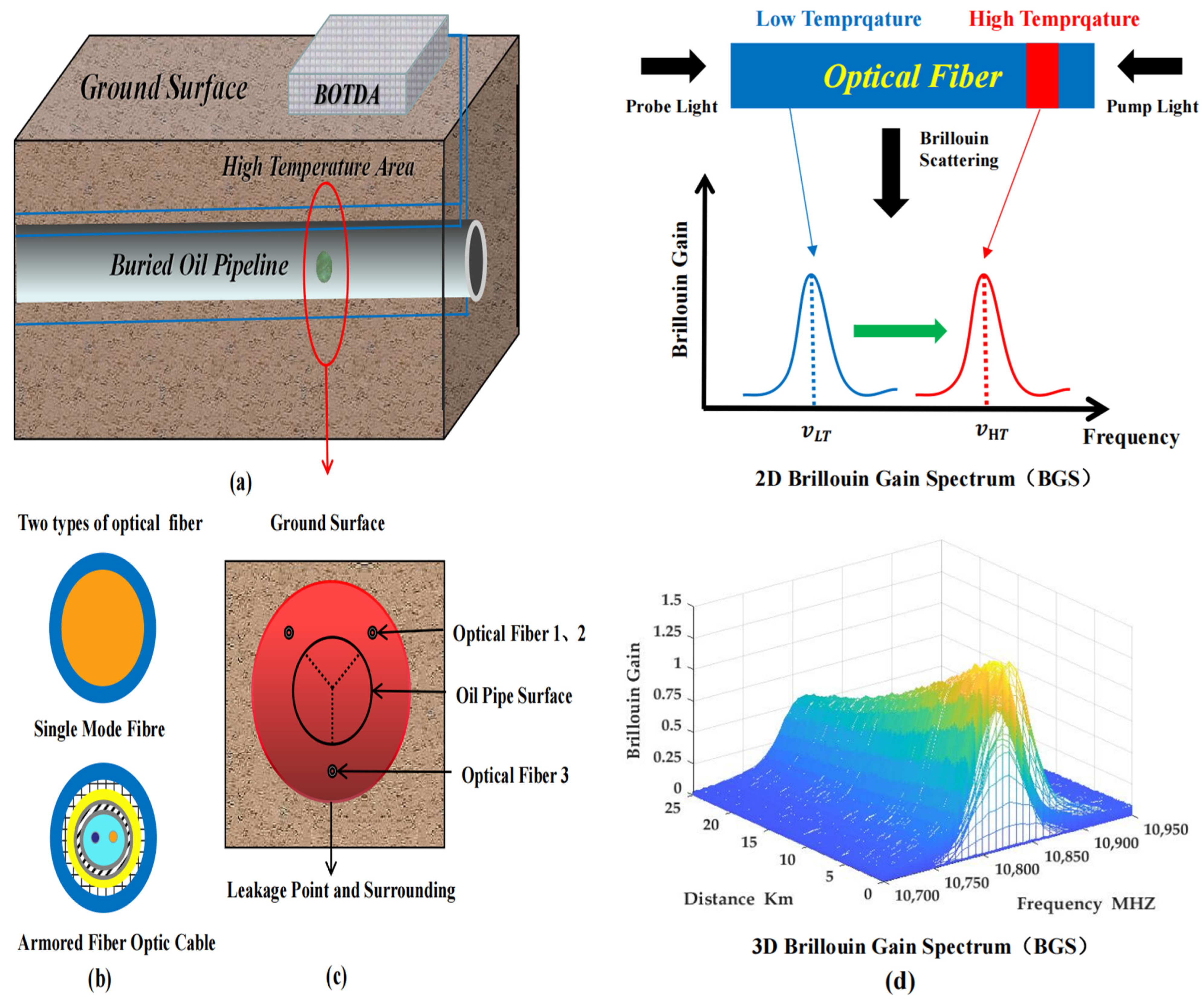
Recently, distributed optical fiber vibration-sensing technology, represented by Brillouin Optical Time Domain Analysis (BOTDA), was applied to oil and nature gas pipeline engineering [4,5,6,7]. When an accident occurs, the temperature near the pipeline will change due to the characteristics of the oil and nature gas pipeline. BOTDA can obtain the Brillouin Gain Spectrum (BGS) at any point of the fiber by scanning the frequency of the optical fiber [8,9,10]. After noise reduction, the BGS can be used to extract the Brillouin Frequency Shift (BFS). The BFS serves as an indicator of temperature, and, as the temperature fluctuates, the BFS changes as well. A field test showed that this change exhibits a positively correlated linear relationship, where a 1 °C change corresponds to a 1–1.1 MHZ change in frequency. BOTDA directly utilizes communication optical fiber cables buried alongside the pipeline as sensors [6], providing advantages such as an extended measurement distance, intrinsic safety, a precise positioning capability, and significant technical benefits [11]. Figure 1 shows a schematic of using BOTDA to detect the temperature of a buried pipeline.

Figure 1.
Schematic of using BOTDA to detect buried pipeline temperature. (a) Using BOTDA to measure the temperature of leaking pipelines; (b) two types of optical fiber; (c) schematic diagram of optic fiber arrangement; and (d) the relationship between pipeline temperature and BGS.
However, due to the long sensing distance of oil and nature gas pipelines, the improvement in sensing resolution, and the rapid increase in system noise and data processing capacity, the traditional Brillouin Spectrum noise reduction processing method faces challenges in meeting the stipulated criteria of the BOTDA sensor system for temperature measurements [12]. Therefore, it becomes imperative to utilize an optimized BGS noise reduction algorithm. This algorithm aims at enhancing the Signal-to-Noise Ratio (SNR) within the BOTDA system, a critical step elucidated in previous works [13,14,15].
1.2. Related Works
In recent years, researchers have chosen to introduce support vector machine methods and design program experiments to optimize the temperature-monitoring techniques in various fields such as oil and gas pipelines, rail transportation, and bridge construction [16,17]. Confronted with the challenges of temperature monitoring in structural engineering, existing research has utilized data analyses and numerical methods to establish multiple linear regression models for optimization [18,19]. In the field of temperature monitoring for oil and gas pipelines, how to use optimization methods to improve the temperature-monitoring performance of the BOTDA system has always been a research hotspot, domestically and internationally.
At present, researchers of the Brillouin Spectrum denoising algorithm take advantage of the characteristics of the BOTDA system’s BGS data points as pixels in the image, and use image-processing algorithms for denoising to improve the SNR of the BOTDA system and enhance the precision of the BFS extraction, so as to obtain more accurate distributed temperature measurement values [20,21,22]. The image-processing algorithm, Non-Local Means (NLM), is a widely used denoising method, which uses the non-local self-similarity of an image to collect the most similar image blocks and perform a weighted average to obtain the current pixel value, so that the denoising effect is greatly improved. In fact, each BGS within the 3D BGS dataset represents a noisy curve following a Lorentzian distribution. The individual pixels in these BGS curves are not isolated; this results in a significant amount of redundancy and similar image patches across the 3D BGS data. Therefore, if only the local area information in the 3D BGS is used for the noise reduction, the final effect will be greatly limited [23,24]. However, the NLM algorithm makes full use of the similarity between different regions in the 3D BGS, and the weighted average of the similar image blocks can better restore the data information, so that the Signal-to-Noise Ratio (SNR) of the system is greatly improved. The details in the image are also preserved. However, with an improvement in the noise level, the NLM algorithm will produce an unsatisfactory denoising effect. The algorithm fails to retain high-frequency detail information such as image contour and texture, resulting in the phenomenon of excessive processing [25].
In recent years, many scholars have improved NLM around the above problems encountered in the process of image processing [26]. In the quest to enhance the Signal-to-Noise Ratio (SNR) within the BGS using an optimized NLM algorithm, Soto introduced an NLM algorithm grounded in noise estimation [27,28]. The experimental findings affirmed the efficacy of this algorithm in effectively eliminating noise from the BOTDA system. The noisy BGS was decomposed into different scales, and the wavelet coefficients of each scale were processed by setting a threshold. The wavelet coefficients (useful signals) greater than the threshold were retained and enhanced, and the wavelet coefficients (noise) less than the threshold were removed. Finally, the image was reconstructed by inverse transform, so as to achieve the purpose of denoising.
In addition, noise levels vary case by case and cannot be measured accurately. IPMs reported that they can achieve a higher SNR than NLM, but they are usually based on noise level estimation [29]. Therefore, many NLM optimization algorithms have been proposed, based on principal component analysis (PCA) [30], noise estimation [27], modified [31], partial window [10,31,32], and signal estimation [33]. Recently, adopting the Grey Wolf algorithm and a neural network to optimize NLM has also become an option [34,35,36]. Table 1 shows the problems existing in the improved BGS optimization algorithm.

Table 1.
Problems existing in the improved BGS optimization algorithm.
1.3. Organization
The remaining parts of this paper are as follows: Section 2 mainly discusses the challenges in addressing the existing algorithm issues. Section 3 illustrates the specific setup and plan for field testing, data preprocessing for the field test data, the methodology for optimizing the research algorithm, and the operating conditions for comparing the new algorithm with other algorithms. Section 4 explains the research cases, comparing the processing effects of the proposed algorithm with those of existing algorithms, including comparisons in terms of visual quality, system signal-to-noise ratio, structural similarity, and time. Section 5 summarizes the research results of the algorithm comparison and provides the conclusions of this study.
2. Problem Description
The above improved algorithms for BGS denoising mainly focus on improving the problems of Euclidean distance and search and similar double Windows, and the lack of related algorithm research on filtering the parameter selection [31]. In the actual situation, due to the inherent characteristics of the BOTDA system, the energy signal at the end of the distributed fiber is small, so it is necessary to ensure the integrity of the local information while denoising. Although great progress has been made in the improvement of non-local mean algorithm problems, there are still the following shortcomings.
- The above algorithms have the problem that the denoising effect and local information processing cannot be taken into account simultaneously.
- Focusing on the processing effect of the image visual quality, SNR improvement, and other aspects, it does not consider the role of the structural similarity of the BGS collected by BOTDA in the subsequent BFS (temperature information) extraction engineering after the processing.
The above improved algorithm can ensure the denoising effect and it will lead to a lack of local information, which makes it difficult to ensure the optimal denoising. This imperfection affects the structural similarity of the BGS and the subsequent extraction of the BFS, resulting in an inability to accurately obtain the fiber temperature value. Therefore, a new optimal denoising algorithm is needed for BGS denoising processing.
3. Materials and Methods
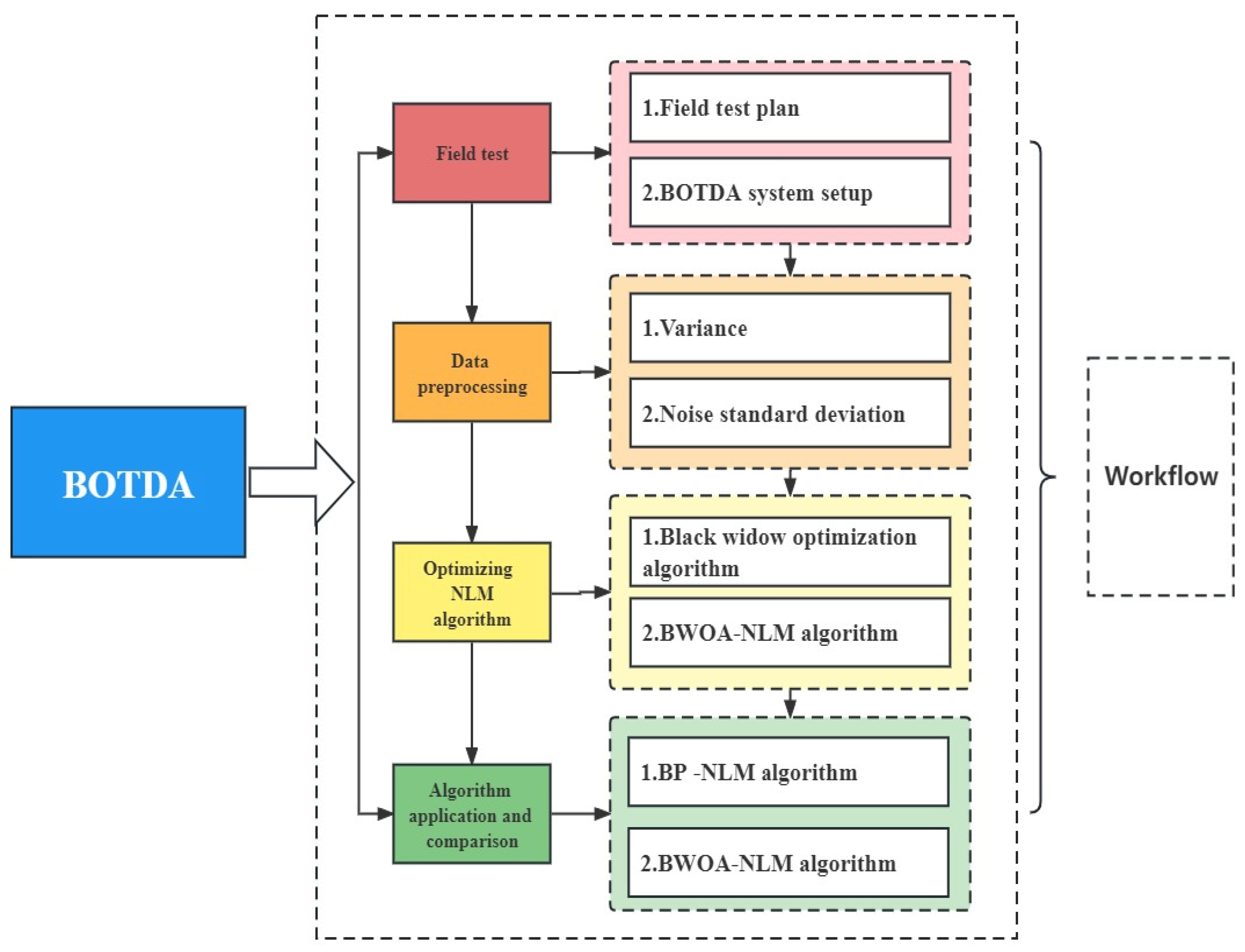
Figure 2 illustrates the workflow of processing an optical fiber BGS using the method proposed in this paper. The workflow comprises four main steps: a field test, data preprocessing, optimizing the NLM algorithm, and the algorithm application and comparison. The details of each step will be discussed in the following sections.
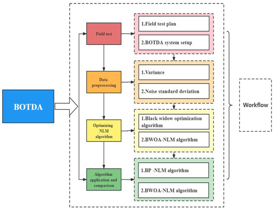
Figure 2.
Workflow of processing optical fiber BGS.
3.1. Field Test
3.1.1. Field Test Plan
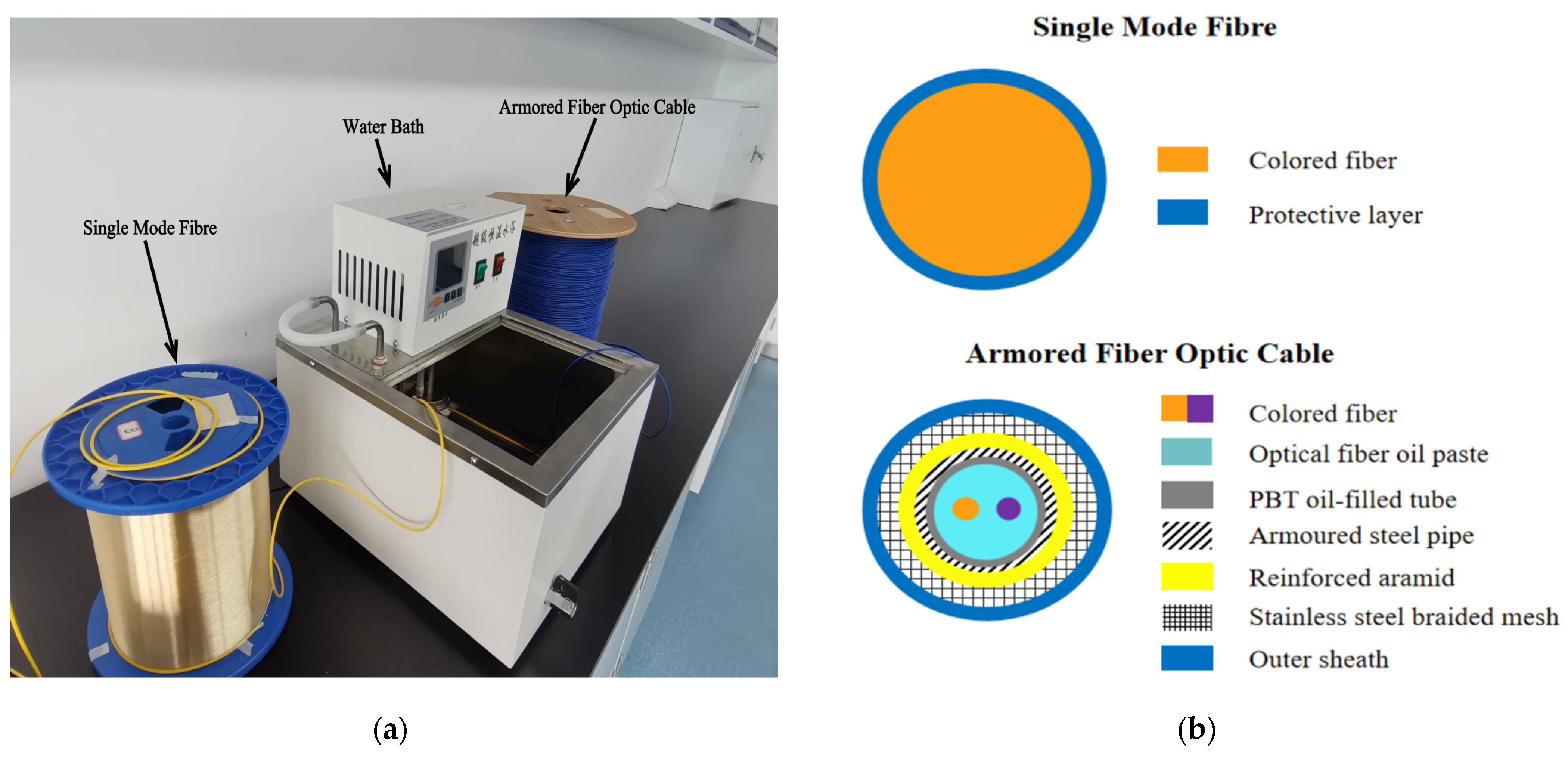
As shown in Figure 3, the field test involves setting up one reel of 24 km single-mode G652 optical fibers, denoted as A, and one reel of a 1 km armored optical cable, denoted as B. In addition, the optical fibers labeled A and B are connected. The total length of the connected optical fiber from reel B to the armored optical cable is set to 25 km.
- The temperature is controlled at 15 °C (the actual temperature is 14.4 °C) using a constant-temperature water bath.
- At a position of 24,950–24,955 m along the connected fiber, the temperature is increased to 50 °C within 1 min (the actual temperature is 49.4 °C) using a constant-temperature water bath. Subsequently, BGS data can be collected.
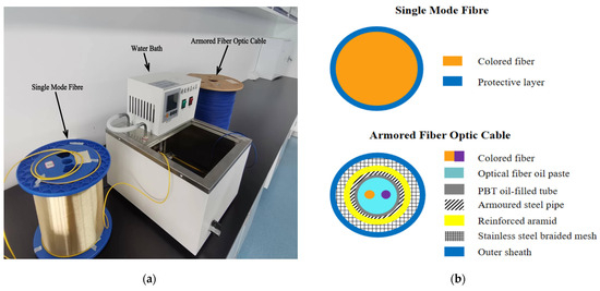
Figure 3.
Field test. (a) A photo of the variable temperature field test setup consisting of optical fibers and a water bath; and (b) the internal structures of two types of optical fibers.
Figure 3.
Field test. (a) A photo of the variable temperature field test setup consisting of optical fibers and a water bath; and (b) the internal structures of two types of optical fibers.
3.1.2. BOTDA System Setup
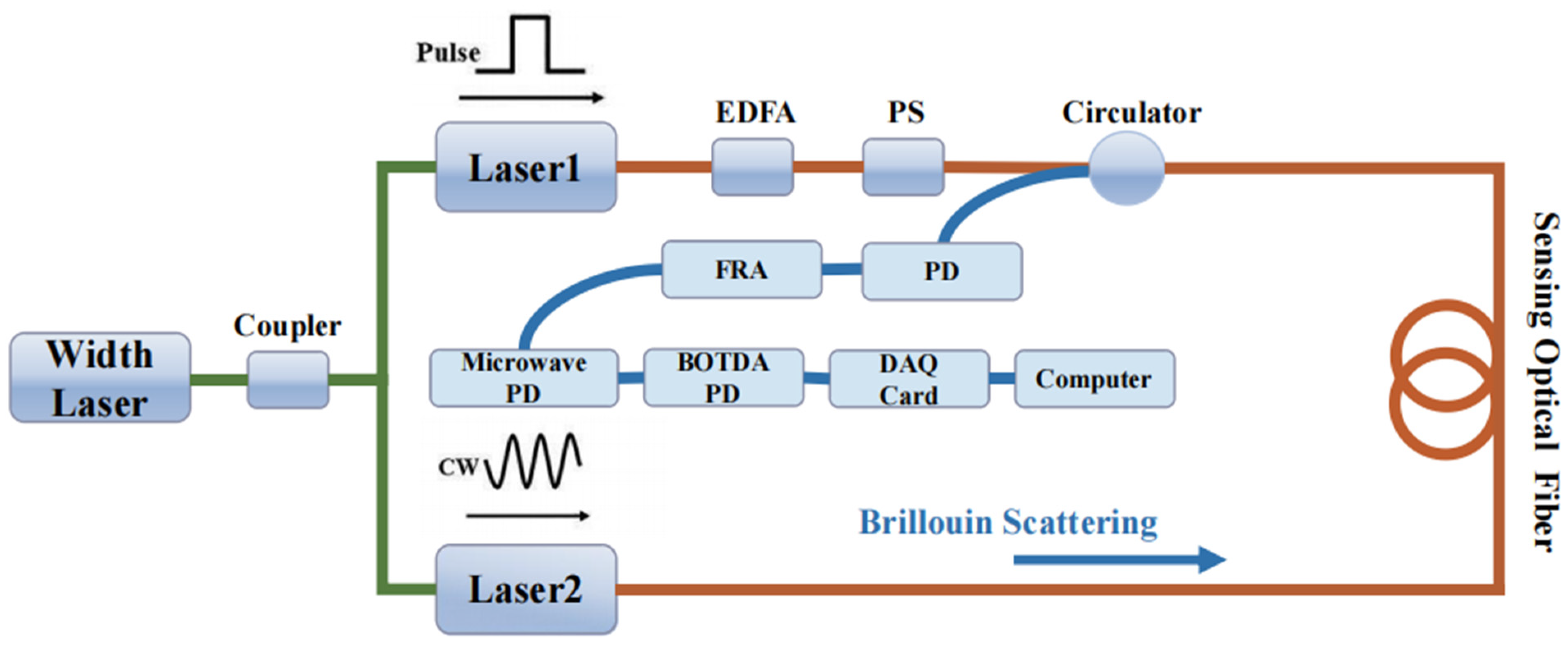
BOTDA (Figure 4) employs a narrow-linewidth laser with a center wavelength of 1550 nm as the light source. The laser emits light, which is then split into two paths by a 50:50 optical coupler.

Figure 4.
Schematic of the BOTDA light path.
One path is modulated by a 50 dB extinction ratio acoustic-optic modulator (AOM) to generate a 1550.12 nm working wavelength pulse pump light with a pulse width of 20 ns. This pump light enters the pump laser module and is amplified by an erbium-doped optical fiber amplifier (EDFA) to achieve a peak power of 20 dBm. Before entering the circulator, the amplified pump light passes through a fiber polarization scrambler (PS) to eliminate the influence of polarization on the pump light and detected light due to Stimulated Brillouin Scattering (SBS) effects.
The other path of light is modulated by a 30 dB extinction ratio electro-optic modulator (EOM) to generate a 1550.2 nm working wavelength detection light, which then enters the detection laser module. The microwave signal’s frequency range is set from 10,700 MHZ to 10,950 MHZ through the upper computer program, ensuring that the detection light is scanned within the Brillouin gain region. To protect the EOM from damage caused by backward-propagating light, an isolator is placed at the output end of the EOM. In the test fiber, the pulse light interacts with the detection light, resulting in an SBS amplification effect. The generated scattered light is converted into an electrical signal (10,700–10,950 MHZ) by a coherent detection module (Photodetector, PD). For signal acquisition convenience, the fiber Raman amplification (FRA) module is first used for gain, followed by the microwave frequency detection (Microwave PD) module scanning. Finally, the BOTDA-PD module is used to detect and capture the Brillouin scattering signal. The system utilizes a data acquisition (DAQ) card for signal acquisition, and computer control of the DAQ card enables data acquisition and processing functionalities.
3.2. Data Preprocessing
In the NLM algorithm, the weight function will affect the processing effect, and the weight function is affected by the smoothing parameter h.
For the BOTDA system, the value of the smoothing parameter h in the NLM algorithm affects its performance. If the value is too large, the denoised image will be excessively smooth, leading to a loss of important details. On the other hand, if the value is too small, although it preserves the details in the image, the denoising effect is not guaranteed.
The selection of the smoothing parameter h depends on the magnitude of the noise standard deviation in the image, and it can be considered as a multiple of the noise standard deviation.
After extracting the noisy BGS image in the field test, the variance δ of the pixel values in the noisy BGS image is computed. The variance δ can be calculated using Equation (1):
where is the number of pixels, is the pixel value, is the pixel value mean.
The noise standard deviation σ is the square root of the variance δ, as shown in Equation (2):
3.3. Optimize NLM Algorithm
To address this issue, BWOA is introduced to control the selection of the smoothing parameter h. The determination of h depends on the noise level present in the image [37,38].
3.3.1. Black Widow Optimization Algorithm
- Initial population
In the algorithm, each potential solution is represented as an individual spider. Each one represents the values of the problem variables. In this study, in order to address the issue, its structure should be regarded as an array.
- 2.
- Movement
As a component of the strategies related to movement, the spider’s motions within the web are simulated using linear and spiral patterns, as outlined in Equation (3) and depicted in Figure 5 [39,40,41].
where represents the spider’s motion when exploring a new spider agent position and is the best, most optimal spider discovered in the previous iteration. The variable is a random float within the range of [0.4, 0.9] and β is a random float within the interval of [−1.0, 1.0], represents the random integer numbers generated from 1 to the size of the maximum of the search spider agents and is the th spider selected, (). Finally, is the current spider.
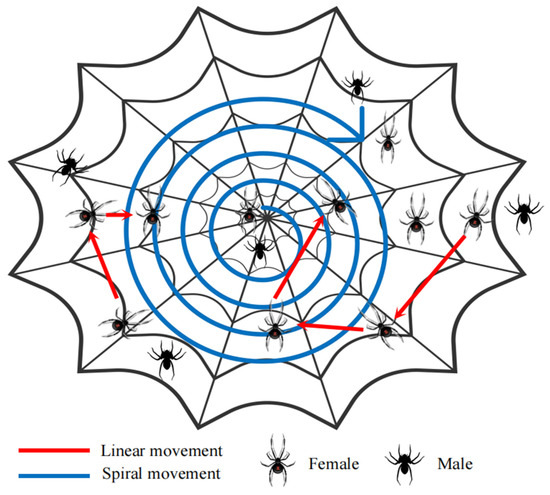
Figure 5.
Black widow spider movement [39].
- 3.
- Pheromone
Pheromones play a crucial role in the courtship and mating behavior of spiders. Male spiders tend to favor female spiders with higher pheromone rates. In the context of this algorithm, the pheromone rate value for the black widow spider is determined using the equation provided in Equation (4) [42,43].
where is the current fitness value of the search spider, is the worst fitness value in the current generation, and is the best fitness value in the current generation. The higher the fitness value, the better the individual’s performance in the environment.
When the pheromone size is less than or equal to 0.3, the individual will be replaced. When female spiders have low pheromone levels, this is indicative of hungry cannibal spiders [44,45]. Consequently, if such low pheromone levels are detected, these specific female spiders will not be selected, and instead, they will be substituted with another candidate. The position update equation is expressed as Equation (5).
where is the female spider with a low pheromone rate that requires updating. and are random integer numbers generated within the range from 1 to the maximum size of the spiders, with , whereas and are the th and th search spider agents selected, and is the best spider found from the previous iteration, .
- 4.
- Cannibalism
In this context, three types of cannibalism are encountered, as outlined in Table 2. The assessment of the spiderlings’ strength or weakness is determined based on their respective fitness values [46,47,48].
Table 2.
Cannibalism categories of black widow spiders.
3.3.2. BWOA-NLM Algorithm
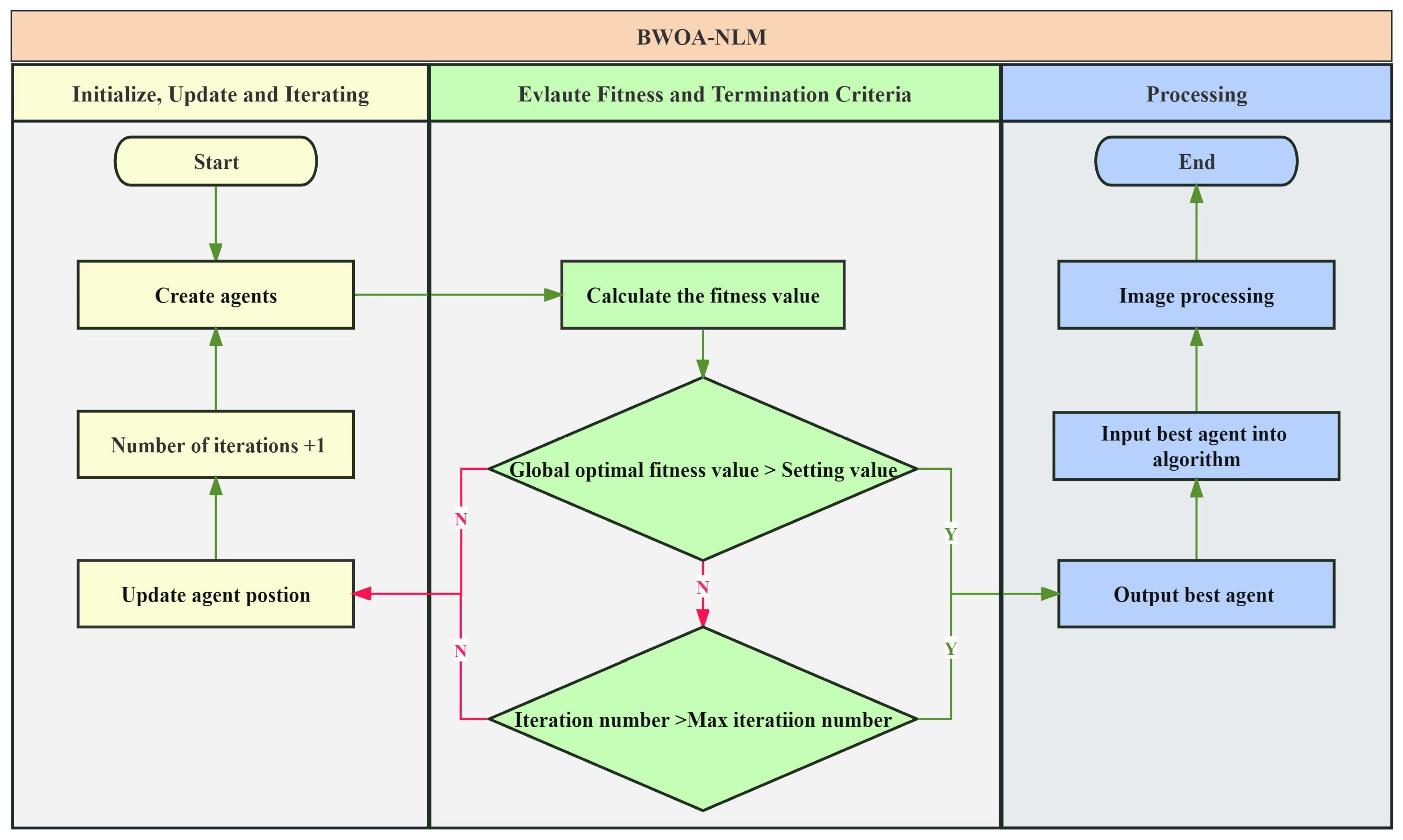
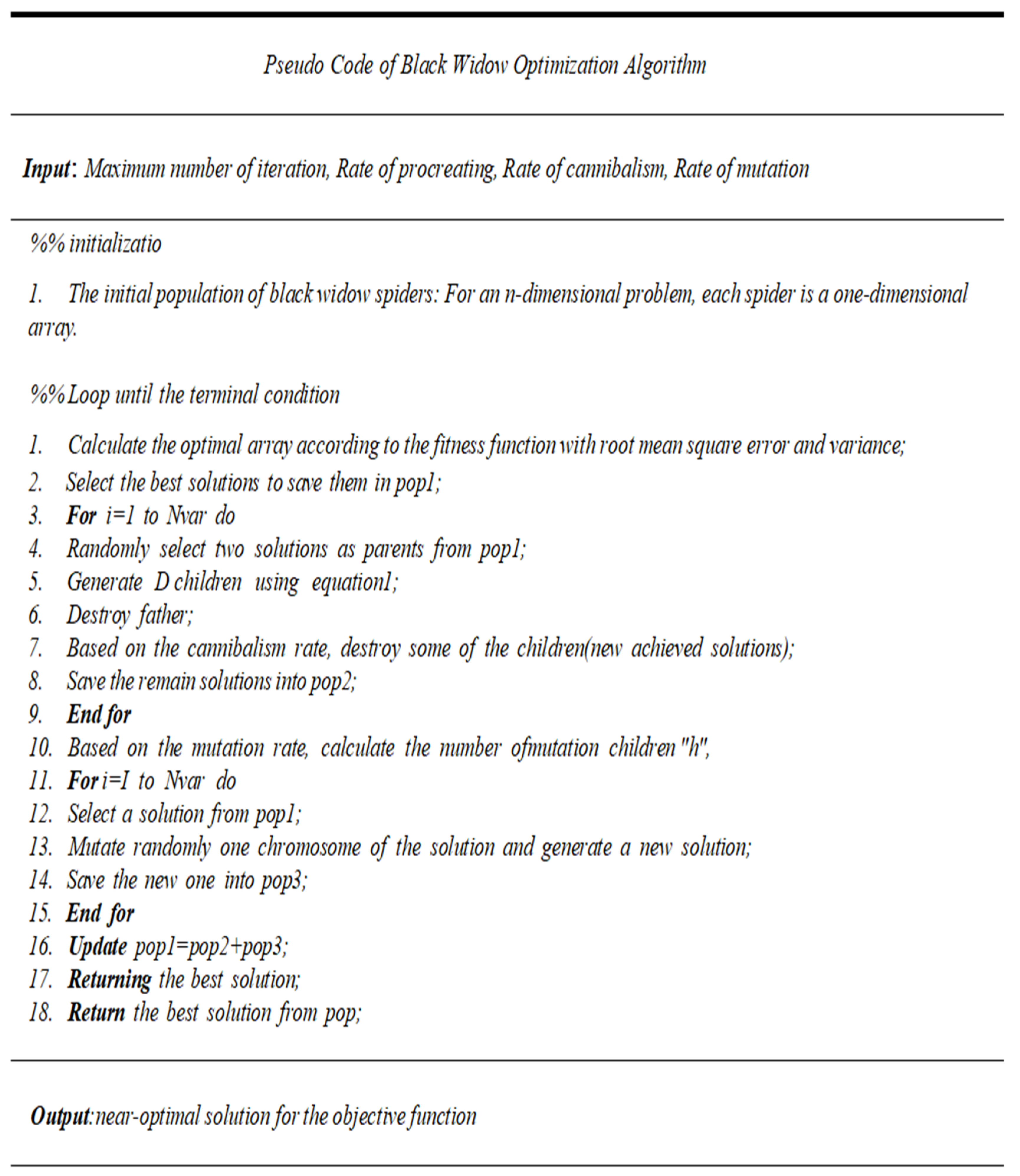
This paper uses the BWOA to select the smoothing parameter h. The steps and Pseudo are shown in Figure 6 and Figure 7.

Figure 6.
Flowchart of BWOA—NLM algorithm.
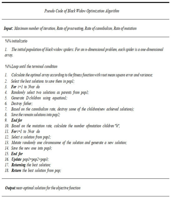
Figure 7.
Pseudo of BWOA algorithm [37].
- Initialization of the spider agents:
The algorithm creates a group of spider agents, where each agent represents a array containing the smoothing parameter h. During initialization, each individual’s h value is set to a random value, ensuring that it falls within 0–100 times the noise standard deviation.
This array (Equation (6)) is defined as follows:
To initiate the optimization algorithm, the fitness of a widow is acquired through an evaluation of the fitness function to start the optimization algorithm, The process commences by generating a candidate widow matrix of size with an initial population of spider agents, then pairs of parents are randomly chosen to engage in the procreation step through mating.
- 2.
- Fitness evaluation
The NLM algorithm is applied to each spider agent h value and its corresponding fitness value is calculated. The fitness of widow is shown in Equation (7):
The fitness function can be based on the SNR and Root Mean Square Error (RMSE) of the processed BGS images, evaluating the quality of the processed images.
The SNR constitutes a pivotal indicator for gauging the measurement precision within a BOTDA system. The SNR can be used to quantitatively evaluate the denoising performance of image-processing algorithms.
The calculation formula for the SNR is shown in Equation (8):
where P is the power of the signal and N is the power of the noise.
RMSE is a statistical measure that assesses the difference between predicted values and actual values. It is used to evaluate the accuracy of prediction models. In fields such as image processing and data analysis, RMSE is commonly employed to gauge the magnitude of the errors between the model predictions and observed data.
The calculation formula for RMSE is shown in Equation (9):
where M is the length of the BGS image, N is the width of the BGS image, is a noisy image, and is a processed image.
- 3.
- Update of individual positions
Based on the computed fitness values, a portion of the top-performing spider agents is selected, and their h values are updated using an information exchange mechanism. The information exchange can involve selecting new h values randomly around the vicinity of the best spider agents. Figure 8 shows the flow.
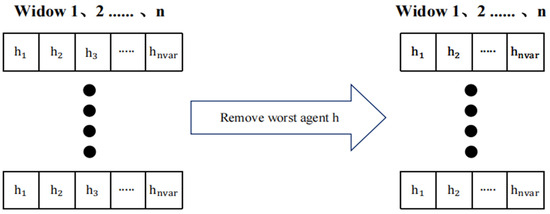
Figure 8.
Update by removing the worst agent in black widow.
- 4.
- Iterative optimization
The algorithm performs multiple iterations, continuously updating the h values of the spider agents and recalculating the fitness function. Through iterative optimization, the spider agents will gradually converge towards h values that lead to better denoising results when processing images.
- 5.
- Termination Criteria
Termination conditions are set when reaching a certain number of iterations or when the fitness function value converges to a specific threshold, to stop the iteration and obtain the optimized h values.
- 6.
- Processing
The best spider agents (the smoothing parameter set h) are substituted into the NLM algorithm for processing.
3.4. Algorithm Application and Comparison
This paper compares the NLM algorithm optimized by the Black Widow Optimization Algorithm (BWOA-NLM) with the NLM algorithm optimized by the Backpropagation neural network (BP-NLM). The BP-NLM algorithm eliminates the process of selecting the smoothing parameter and instead utilizes a pre-trained neural network to filter images.
Each algorithm is independently run 400 times to process the collected BGS. The operating conditions are shown in Table 3.
Table 3.
The operating conditions of algorithm.
4. Results and Discussion
4.1. Visual Quality
4.1.1. 3D BGS
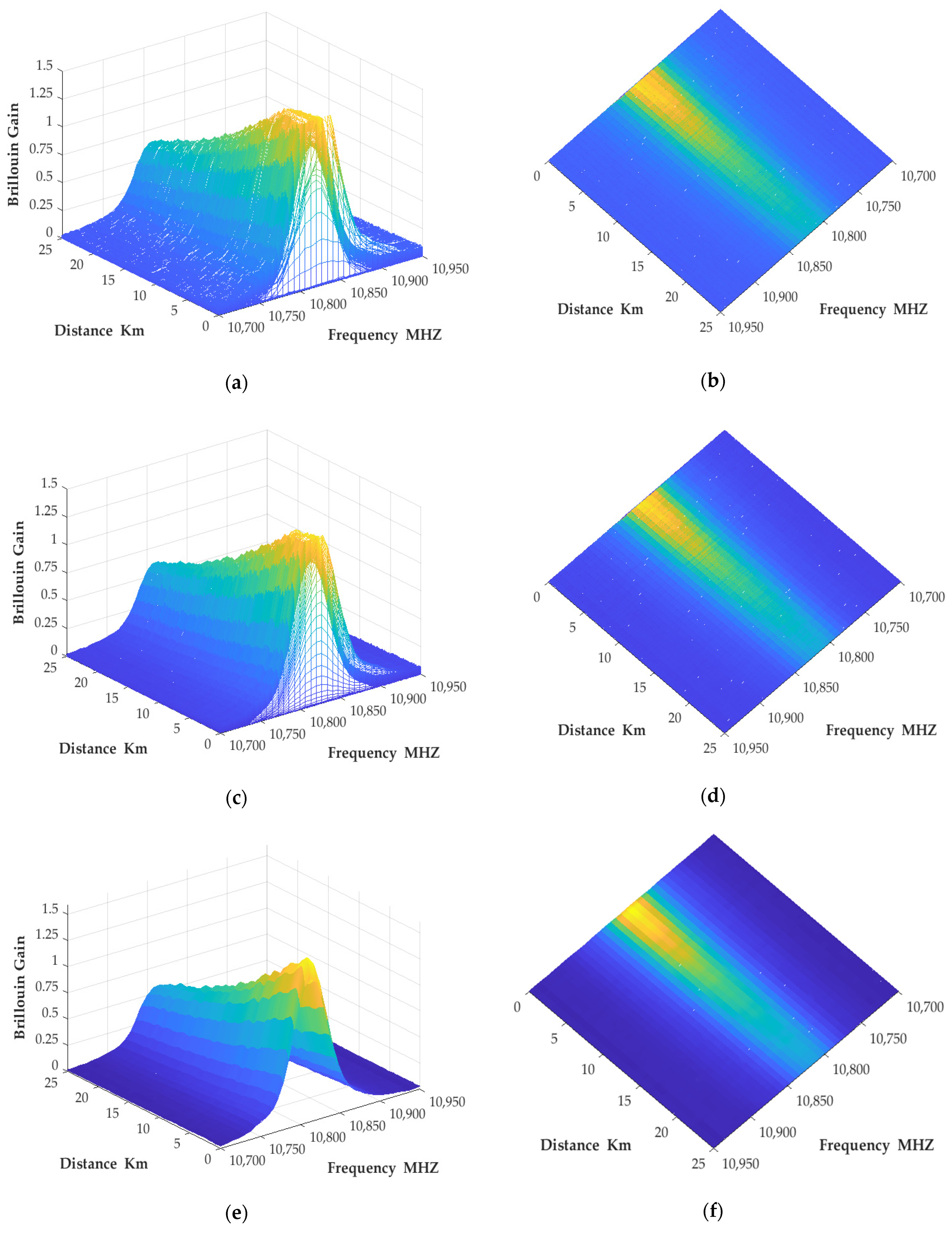
As shown in Figure 9, it is visually evident that the original BGS contains numerous spikes and is contaminated with noise. However, after applying the BWOA-NLM algorithm, the noise is reduced, resulting in a smoother spectral profile with clearer BGS contours. Additionally, the BWOA-NLM algorithm shows a better denoising performance compared to the BP-NLM algorithm.

Figure 9.
Three-dimensional BGS. (a) The noisy BGS; (b) the noisy BGS (local details); (c) the BGS processed by the BP-NLM algorithm; (d) the BGS processed by the BP-NLM algorithm (local details); (e) the BGS processed by the BWOA-NLM algorithm; and (f) the BGS processed by the BWOA-NLM algorithm (local details).
4.1.2. Fixed Frequency and Position
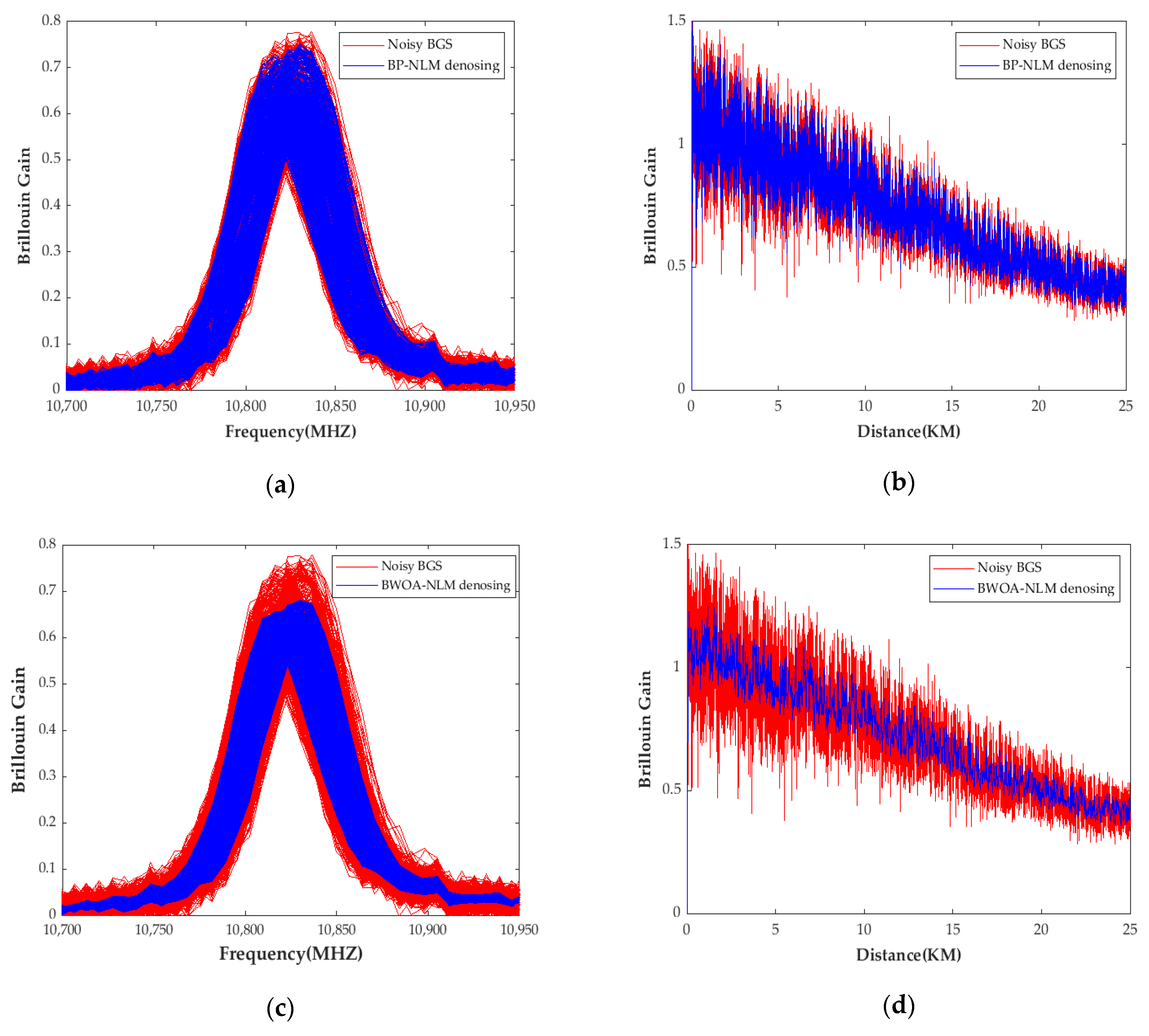
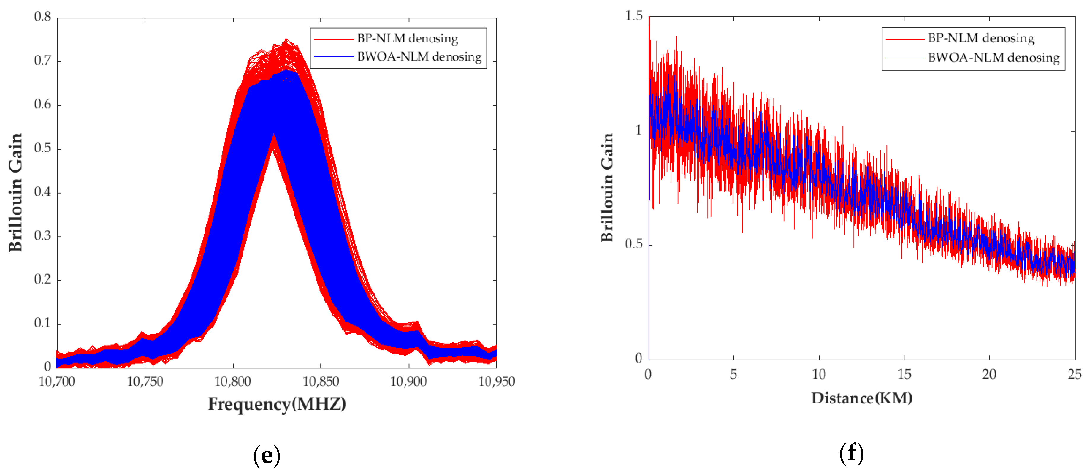
To further demonstrate the denoising capabilities of the image-processing algorithms, the noisy BGS curves are extracted at 25 km of the optical fiber with a scanning frequency of 10,840 MHZ.
The BWOA-NLM and BP-NLM algorithms are used for processing. From Figure 10, it is visually evident that both algorithms effectively remove a certain amount of noise from the data. After the denoising process, the random jitter on the curves is reduced, presenting a more ideal Lorentzian-shaped curve. Additionally, the BWOA-NLM algorithm shows a better denoising performance compared to the BP-NLM algorithm.

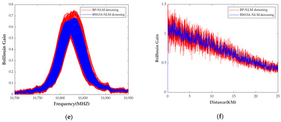
Figure 10.
Fixed frequency and fixed position of the BGS. (a,b) BP-NLM algorithm; (c,d) BWOA-NLM algorithm; and (e,f) BP-NLM algorithm and BOWA-NLM algorithm.
4.2. System SNR
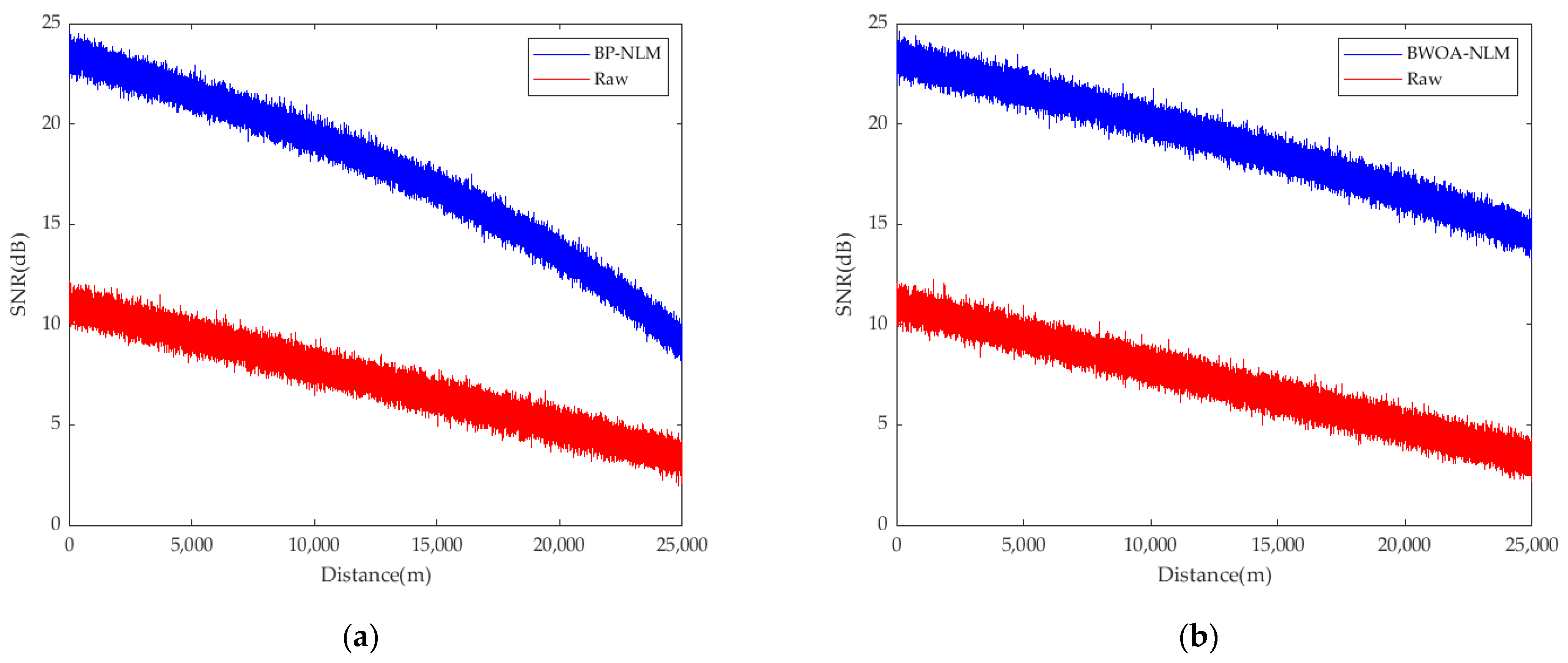
In Figure 11, a comparison is made between the calculated SNR of the raw data and the SNR after processing with the two denoising algorithms. The red solid line represents the SNR of the raw data, while the blue solid line represents the SNR after applying the two denoising algorithms.
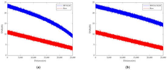
Figure 11.
The comparison of SNR before and after denoising. (a) BP-NLM algorithm and (b) BWOA-NLM algorithm.
From Table 4, it can be observed that the SNR of the raw data (raw) is at its minimum at the fiber end (25 km), with a value of approximately 3 dB. After applying the two different denoising algorithms, the system’s SNR is improved to some extent. Among them, the BWOA-NLM algorithm shows the most significant improvement, with an SNR increase of about 13.3 dB, demonstrating an excellent denoising performance, even at the fiber end.
Table 4.
The SNR at different positions of the fiber.
4.3. Structural Similarity and Time
Full Width at Half Maximum (FWHM) is related to the pulse width of an optical signal, as shown in Table 5. In the BOTDA system, with an increasing distance of the fiber, the function of the pump light is gradually attenuated and the SBS effect is further weakened, thus showing a large frequency uncertainty at the end of the fiber. However, near the fiber heating spot, the BFS obtained by the BWOA-NLM denoising algorithm is smoother, and its frequency uncertainty is greatly reduced. The frequency uncertainty is shortened from 8 MHZ to 3 MHZ (the optical pulse width used in this field test is 20 ns) after the denoising processing, and the FWHM of BWOA-NLM matches better with the FWHM of BP-NLM. It can be seen that the new image-processing algorithm effectively removes the noise in the BGS, while preserving the shape and basic characteristics of the BGS.
Table 5.
FWHW corresponding to different light pulses.
Root Mean Square Error (RMSE) and Sum of Squared Errors (SSE) are used to measure the degree of data fitting. The RMSE is the standard deviation of the average error, while the SSE is the total sum of all the squared errors. A smaller RMSE and SSE indicate a better fit between the predicted BFS and the actual BFS corresponding to the processed background signal, meaning that the error between the predicted and actual values is smaller. Therefore, when evaluating the degree of data fitting, algorithms with a smaller RMSE and SSE are usually preferred. As shown in Table 6, the RMSE and SSE of BP-NLM are smaller than those of BP-NLM; the RMSE is reduced by 0.028 and the SSE is reduced by 0.067.
Table 6.
Comparison of data processed by the two algorithms.
The operation time is one of the important indicators that reflects the actual processing capability of an algorithm. The BWOA-NLM algorithm takes an additional 0.8 s.
The Root Mean Square Error (RMSE), Sum of Squared Errors (SSE), Full Width at Half Maximum (FWHM), and processing time for both algorithms are shown in Table 6.
Therefore, the BWOA-NLM algorithm can effectively suppress the noise of the system and better maintain its detail components.
5. Conclusions
This paper proposed an improved algorithm, which can extract the BFS better in follow-up works and improve the reliability of the BOTDA system for pipeline temperature monitoring.
- This article proposed a local mean algorithm optimized by the black widow algorithm, which can maintain the detailed information of the Brillouin Gain Spectrum (BGS) while removing noise.
- Through a series of field tests, it was verified that the proposed method had better advantages than the BP-NLM algorithm in terms of detail preservation and noise suppression. The BWOA-NLM algorithm improved the Signal-to-Noise Ratio of the BGS by 11–12.9 dB, and, compared to the BP-NLM algorithm, the BWOA-NLM algorithm still maintained a level of 10.3 dB for the BGS Signal-to-Noise Ratio at the fiber end (25 km), which was about 3 dB higher than that of the BP-NLM algorithm.
- Compared to the BP-NLM algorithm, the BWOA-NLM algorithm improved the Root Mean Square Error (RMSE), Sum of Squared Errors (SSE), and Full Width at Half Maximum (FWHM) data by 9.4%, 12.5%, and 10%, respectively. The processing performance reflected that the BWOA-NLM algorithm could better extract the BFS and improve the reliability of the BOTDA system in pipeline temperature monitoring. However, in terms of the processing time, the BWOA-NLM algorithm took an additional 0.8 s. The difference between the two was significant, and the processing time of the BWOA-NLM algorithm still needs further improvement.
- Future research should aim to accurately fit BGS curve data for temperature detection, create a database for identifying temperature anomalies, and enable the secure monitoring of on-site pipeline systems.
Author Contributions
Conceptualization, F.L., B.H. and R.S.; methodology, F.L. and B.H.; software, F.L.; validation, F.L.; formal analysis, F.L., R.S., B.W. and W.H.; writing—original draft preparation, F.L.; writing—review and editing, F.L., B.W., B.H. and Z.C.; supervision, B.H. and B.Z.; funding acquisition, B.H. and B.Z. All authors have read and agreed to the published version of the manuscript.
Funding
This research was funded by the Zhejiang Province Key Research and Development Plan (No. 2021C03152), Zhejiang New Talent Plan of Student’s Technology and Innovation Program (No. 2022R411A022), Zhejiang Ocean University Science and Technology Project (No. 1102106412202).
Data Availability Statement
Not applicable.
Conflicts of Interest
The authors declare no conflict of interest.
References
- Li, Y.; Kuang, Z.; Fan, Z.; Shuai, J. Evaluation of the safe separation distances of hydrogen-blended natural gas pipelines in a jet fire scenario. Int. J. Hydrogen Energy 2023, 48, 18804–18815. [Google Scholar] [CrossRef]
- Mokhtari, M.; Melchers, R.E. Reliability of the conventional approach for stress/fatigue analysis of pitting corroded pipelines—Development of a safer approach. Struct. Saf. 2020, 85, 101943. [Google Scholar] [CrossRef]
- Li, X.; Liu, R.; Jiang, H.; Yu, P.; Liu, X. Numerical investigation on the melting characteristics of wax for the safe and energy-efficiency transportation of crude oil pipelines. Meas. Sens. 2020, 10, 100022. [Google Scholar] [CrossRef]
- Zha, J.; Meng, Y.; Li, D.; Yin, H.; Wang, D.; Yu, W. Determination of average times for Brillouin optical time domain analysis sensor denoising by non-local means filtering. Opt. Commun. 2018, 426, 648–653. [Google Scholar] [CrossRef]
- Li, Q.; Shi, Y.; Lin, R.; Qiao, W.; Ba, W. A novel oil pipeline leakage detection method based on the sparrow search algorithm and CNN. Measurement 2022, 204, 112122. [Google Scholar] [CrossRef]
- Bao, X.; Chen, L. Recent progress in distributed fiber optic sensors. Sensors 2012, 12, 8601–8639. [Google Scholar] [CrossRef]
- Claus, M. On continuity in risk-averse bilevel stochastic linear programming with random lower level objective function. Oper. Res. Lett. 2021, 49, 412–417. [Google Scholar] [CrossRef]
- Mirzaei, A.; Bahrampour, A.; Taraz, M.; Bahrampour, A.; Bahrampour, M.; Foroushani, S.A. Transient response of buried oil pipelines fiber optic leak detector based on the distributed temperature measurement. Int. J. Heat Mass Transf. 2013, 65, 110–122. [Google Scholar] [CrossRef]
- Wang, F.; Liu, Z.; Zhou, X.; Li, S.; Yuan, X.; Zhang, Y.; Shao, L.; Zhang, X. Oil and gas pipeline leakage recognition based on distributed vibration and temperature information fusion. Results Opt. 2021, 5, 100131. [Google Scholar] [CrossRef]
- Datta, A.; Mamidala, H.; Venkitesh, D.; Srinivasan, B. Reference-free real-time power line monitoring using distributed anti-Stokes Raman thermometry for smart power grids. IEEE Sens. J. 2019, 20, 7044–7052. [Google Scholar] [CrossRef]
- Laarossi, I.; Quintela-Incera, M.Á.; López-Higuera, J.M. Comparative experimental study of a high-temperature raman-based distributed optical fiber sensor with different special fibers. Sensors 2019, 19, 574. [Google Scholar] [CrossRef]
- Li, J.; Zeng, K.; Yang, G.; Wang, L.; Mi, J.; Wan, L.; Tang, M.; Liu, D. High-fidelity denoising for differential pulse-width pair brillouin optical time domain analyzer based on block-matching and 3D filtering. Opt. Commun. 2022, 525, 128866. [Google Scholar] [CrossRef]
- Zhang, M.; Guo, Y.; Xie, Q.; Zhang, Y.; Wang, D.; Chen, J. Defect identification for oil and gas pipeline safety based on autonomous deep learning network. Comput. Commun. 2022, 195, 14–26. [Google Scholar] [CrossRef]
- Xu, Z.; Zhao, L. Accurate and ultra-fast estimation of Brillouin frequency shift for distributed fiber sensors. Sens. Actuators A Phys. 2020, 303, 111822. [Google Scholar] [CrossRef]
- Nikles, M.; Thevenaz, L.; Robert, P.A. Brillouin gain spectrum characterization in single-mode optical fibers. J. Light. Technol. 1997, 15, 1842–1851. [Google Scholar] [CrossRef]
- Ni, Y.; Hua, X.; Fan, K.; Ko, J. Correlating modal properties with temperature using long-term monitoring data and support vector machine technique. Eng. Struct. 2005, 27, 1762–1773. [Google Scholar] [CrossRef]
- Ni, Y.; Zhou, H.; Ko, J. Generalization capability of neural network models for temperature-frequency correlation using monitoring data. J. Struct. Eng. 2009, 135, 1290–1300. [Google Scholar] [CrossRef]
- Tan, X.; Chen, W.; Wang, L.; Yang, J. The impact of uneven temperature distribution on stability of concrete structures using data analysis and numerical approach. Adv. Struct. Eng. 2021, 24, 279–290. [Google Scholar] [CrossRef]
- Tan, X.; Chen, W.; Wu, G.; Wang, L.; Yang, J. A structural health monitoring system for data analysis of segment joint opening in an underwater shield tunnel. Struct. Health Monit. 2020, 19, 1032–1050. [Google Scholar] [CrossRef]
- Zeng, W.; Lu, X. Region-based non-local means algorithm for noise removal. Electron. Lett. 2011, 47, 1125–1127. [Google Scholar] [CrossRef]
- Zhang, Y.; Lu, Y.; Zhang, Z.; Wang, J.; He, C.; Wu, T. Noise reduction by Brillouin spectrum reassembly in Brillouin optical time domain sensors. Opt. Lasers Eng. 2020, 125, 105865. [Google Scholar] [CrossRef]
- Zhao, S.; Cui, J.; Wu, Z.; Tan, J. Accuracy improvement in OFDR-based distributed sensing system by image processing. Opt. Lasers Eng. 2020, 124, 105824. [Google Scholar] [CrossRef]
- Garmire, E. Perspectives on stimulated Brillouin scattering. New J. Phys. 2017, 19, 011003. [Google Scholar] [CrossRef]
- Ruano, P.N.; Zhang, J.; Melati, D.; González-Andrade, D.; Le Roux, X.; Cassan, E.; Marris-Morini, D.; Vivien, L.; Lanzillotti-Kimura, N.D.; Alonso-Ramos, C. Genetic optimization of Brillouin scattering gain in subwavelength-structured silicon membrane waveguides. Opt. Laser Technol. 2023, 161, 109130. [Google Scholar] [CrossRef]
- Zheng, H.; Sun, S.; Qin, Y.; Xiao, F.; Dai, C. Extraction of Brillouin frequency shift from Brillouin gain spectrum in Brillouin distributed fiber sensors using K nearest neighbor algorithm. Opt. Fiber Technol. 2022, 71, 102903. [Google Scholar] [CrossRef]
- Xu, Z.-N.; Zhao, L.-J.; Qin, H. Selection of spectrum model in estimation of Brillouin frequency shift for distributed optical fiber sensor. Optik 2019, 199, 163355. [Google Scholar] [CrossRef]
- Soto, M.A.; Ramírez, J.A.; Thévenaz, L. Optimizing image denoising for long-range Brillouin distributed fiber sensing. J. Light. Technol. 2017, 36, 1168–1177. [Google Scholar] [CrossRef]
- Soto, M.A.; Ramirez, J.A.; Thévenaz, L. Intensifying the response of distributed optical fibre sensors using 2D and 3D image restoration. Nat. Commun. 2016, 7, 10870. [Google Scholar] [CrossRef]
- Chen, Y.; Zhu, P.; Yin, Y.; Wu, M.; Yu, K.; Feng, L.; Chen, W. Objective assessment of IPM denoising quality of φ-OTDR signal. Measurement 2023, 214, 112775. [Google Scholar] [CrossRef]
- Qian, X.; Jia, X.; Wang, Z.; Zhang, B.; Xue, N.; Sun, W.; He, Q.; Wu, H. Noise level estimation of BOTDA for optimal non-local means denoising. Appl. Opt. 2017, 56, 4727–4734. [Google Scholar] [CrossRef]
- Malakzadeh, A.; Didar, M.; Mansoursamaei, M. SNR enhancement of a Raman distributed temperature sensor using partial window-based non local means method. Opt. Quantum Electron. 2021, 53, 147. [Google Scholar] [CrossRef]
- Okamoto, T.; Iida, D.; Oshida, H. Vibration-induced beat frequency offset compensation in distributed acoustic sensing based on optical frequency domain reflectometry. J. Light. Technol. 2019, 37, 4896–4901. [Google Scholar] [CrossRef]
- Wu, M.; Chen, Y.; Zhu, P.; Chen, W. NLM Parameter Optimization for φ-OTDR Signal. J. Light. Technol. 2022, 40, 6045–6051. [Google Scholar] [CrossRef]
- Huang, Q.; Shi, H.; Huang, C.; Sun, J. Improvement of response speed and precision of distributed Brillouin optical fiber sensors using neural networks. Opt. Laser Technol. 2023, 167, 109705. [Google Scholar] [CrossRef]
- Kim, S.H.; Koo, G.; Jeong, J.J.; Kim, S.W. An adjusting-block based convex combination algorithm for identifying block-sparse system. Signal Process. 2018, 143, 1–6. [Google Scholar] [CrossRef]
- Rajakumar, S.; Sreedhar, P.S.S.; Kamatchi, S.; Tamilmani, G. Gray wolf optimization and image enhancement with NLM Algorithm for multimodal medical fusion imaging system. Biomed. Signal Process. Control 2023, 85, 104950. [Google Scholar] [CrossRef]
- Hayyolalam, V.; Kazem, A.A.P. Black widow optimization algorithm: A novel meta-heuristic approach for solving engineering optimization problems. Eng. Appl. Artif. Intell. 2020, 87, 103249. [Google Scholar] [CrossRef]
- Houssein, E.H.; Helmy, B.E.-D.; Oliva, D.; Elngar, A.A.; Shaban, H. A novel black widow optimization algorithm for multilevel thresholding image segmentation. Expert Syst. Appl. 2021, 167, 114159. [Google Scholar] [CrossRef]
- Peña-Delgado, A.F.; Peraza-Vázquez, H.; Almazán-Covarrubias, J.H.; Torres Cruz, N.; García-Vite, P.M.; Morales-Cepeda, A.B.; Ramirez-Arredondo, J.M. A novel bio-inspired algorithm applied to selective harmonic elimination in a three-phase eleven-level inverter. Math. Probl. Eng. 2020, 2020, 8856040. [Google Scholar] [CrossRef]
- Xu, G.; Wang, X. Support vector regression optimized by black widow optimization algorithm combining with feature selection by MARS for mining blast vibration prediction. Measurement 2023, 218, 113106. [Google Scholar] [CrossRef]
- Vijayakumar, S.; Suresh, P. Lean based cycle time reduction in manufacturing companies using black widow based deep belief neural network. Comput. Ind. Eng. 2022, 173, 108735. [Google Scholar] [CrossRef]
- Hu, G.; Du, B.; Wang, X.; Wei, G. An enhanced black widow optimization algorithm for feature selection. Knowl.-Based Syst. 2022, 235, 107638. [Google Scholar] [CrossRef]
- Chauhan, A.; Prakash, S. Comparison and performance analysis of pheromone value and cannibalism based black widow optimisation approaches for modelling and parameter estimation of solar photovoltaic mathematical models. Optik 2022, 259, 168943. [Google Scholar] [CrossRef]
- Kanna, P.R.; Santhi, P. Hybrid intrusion detection using mapreduce based black widow optimized convolutional long short-term memory neural networks. Expert Syst. Appl. 2022, 194, 116545. [Google Scholar] [CrossRef]
- Li, J.; Yan, Y.; Yu, H.; Peng, X.; Zhang, Y.; Hu, W.; Duan, Z.; Wang, X.; Liang, S. Isolation and identification of a sodium channel-inhibiting protein from eggs of black widow spiders. Int. J. Biol. Macromol. 2014, 65, 115–120. [Google Scholar] [CrossRef] [PubMed]
- Fu, Y.; Hou, Y.; Chen, Z.; Pu, X.; Gao, K.; Sadollah, A. Modelling and scheduling integration of distributed production and distribution problems via black widow optimization. Swarm Evol. Comput. 2022, 68, 101015. [Google Scholar] [CrossRef]
- Rodríguez, A.O.; Ruiz, M.G.A.; Bénard-Valle, M.; Neri-Castro, E.; Rodríguez, F.O.; Alagón, A. Neutralization of black widow spider (Latrodectus mactans) venom with rabbit polyclonal serum hyperimmunized with recombinant alpha-latrotoxin fragments. Biochimie 2022, 201, 55–62. [Google Scholar] [CrossRef]
- Sivalinghem, S.; Mason, A.C. Function of structured signalling in the black widow spider Latrodectus hesperus. Anim. Behav. 2021, 179, 279–287. [Google Scholar] [CrossRef]


Disclaimer/Publisher’s Note: The statements, opinions and data contained in all publications are solely those of the individual author(s) and contributor(s) and not of MDPI and/or the editor(s). MDPI and/or the editor(s) disclaim responsibility for any injury to people or property resulting from any ideas, methods, instructions or products referred to in the content. |
© 2023 by the authors. Licensee MDPI, Basel, Switzerland. This article is an open access article distributed under the terms and conditions of the Creative Commons Attribution (CC BY) license (https://creativecommons.org/licenses/by/4.0/).