Distribution Network Reconfiguration Using Chaotic Particle Swarm Chicken Swarm Fusion Optimization Algorithm

Abstract

Aiming at the problems of traditional optimization algorithms for reconfiguring distribution networks, which easily fall into a local optimum, have difficulty finding a global optimum, and suffer from low computational efficiency, the proposed algorithm named Chaotic Particle Swarm Chicken Swarm Fusion Optimization (CPSCSFO) is used to optimize the reconfiguration of the distribution network with distributed generation (DG). This article works to solve the problems mentioned above from the following three aspects: Firstly, chaotic formula is used to improve the initialization of the particles and optimize the optimal position. This increases individual randomness while avoiding local optimality for inert particles. Secondly, chicken swarm optimization (CSO) and particle swarm optimization (PSO) are combined. The multi-population nature of the CSO algorithm is used to increase the global search capability, and, at the same time, the information exchange between groups is completed to extend the particle search range, which ensures the independence and excellence of each particle group. Thirdly, the node hierarchy method is introduced to calculate the power flow. The branching loop matrix and the node hierarchy strategy are used to detect the network topology. In this way, improper solutions can be reduced, and the efficiency of the algorithm can be improved. This paper has demonstrated better performance by CPSCSFO based on simulation results. The network loss has been reduced and the voltage level of each node in the optimal reconfiguration with distributed power supply has been improved; the network loss in the optimal reconfiguration with DG is 69.59% lower than that reconfiguration before. The voltage level of each node is increased, the minimum node voltage is increased by 3.44% and a better convergence speed is presented. As a result, the quality of network operation and the distribution network is greatly improved and provides guidance for building a safer, more economical and reliable distribution network.

1. Introduction

With the continuous expansion of large-scale power grids, people’s demands on indicators such as the quality and reliability of power operation are increasing [1,2]. To solve the problems of complex operation, high investment and environmental pollution of traditional power generation technology, distributed power generation technology has been introduced. It can not only save investment and reduce losses but also improve the reliability and flexibility of power grid operation [3,4]. At the same time, combining this technology with a large-scale power grid can promote the development of the power grid. It paves the way for the development of clean energy [5].

The optimization and reconfiguration of distribution networks involve non-linear, multi-dimensional and multi-objective functions [6]. Moreover, the reconstruction process should satisfy the constraints of voltage, current and power flow. The network topology is reconfigured by manipulating the on-off state of the switch. Then, the global optimal solution can be found quickly to meet the requirements of low network operation cost and high power quality [7].

Currently, the traditional optimization methods used for distribution network reconfiguration are mainly divided into mathematical optimization methods [8,9] and heuristic algorithms [10]. However, with access to large-scale power grids, the traditional optimization algorithms are no longer applicable. Many scientists are turning to the study of artificial intelligence algorithms. In Reference [11], to get rid of the pre-particles trapped in the local optimum, the genetic and mutation operations of the genetic algorithm are combined with the quantum particle swarm optimization algorithm. The method implements probabilistic evolution of the particles and thus improves the diversity of the population. Reference [12] introduces multiple voltage levels to improve the coordination among voltage levels. This improves the optimal allocation of power grid resources. Based on the Cuckoo algorithm, a simulated annealing algorithm is added to improve convergence accuracy and global search capability, but the system does not consider the reconfiguration of the distribution network with DG. Reference [13] improves the Grey Wolf algorithm and introduces the ordered ring network coding method. It significantly reduces the peak value of the solution space for distribution network reconfiguration and improves the optimization efficiency of the algorithm. Reference [14] improves the group search algorithm by using fuzzy theory, which extends the simple search space to a two-dimensional search space. It considers the switching state and the photovoltaic power as two decision variables. The algorithm is applied to the reconfiguration of the distribution grid to improve the efficiency of the optimization path. Reference [15] proposes an IHBO for identifying the optimum PDSR, which is combined with finding the optimal placement and sizing of numerous DG units. The IHBO is designed to provide electricity with minimal power losses and maximum voltage stability. Reference [16] presents an Enhanced Marine Predators Algorithm (EMPA) for simultaneous optimal distribution system reconfigurations (DSRs) and distributed generation (DG) addition. The reconfiguration is performed in IEEE 33-bus and large-scale 137-bus distribution networks, respectively. The simulation outputs reveal significant improvements in the standard MPA and demonstrate the superiority and effectiveness of the proposed EMPA compared to other reported results by recent algorithms for DSRs associated with DG integration. In [17], a new implementation of the Artificial Ecosystem Optimizer (AEO) technique is developed for distributed generations (DGs) and capacitor allocation, considering the Reconfiguration of Power Distribution Systems (RPDS). By comparing it to other intelligent algorithms, it surpasses the other algorithms in terms of obtaining the best, mean, worst and standard deviations. However, this algorithm has not been applied to large-scale distribution systems. Reference [18] proposes an improved Heap-based algorithm to enhance the performance of a recently published technique called Heap-based optimizer (HO). The simulation results demonstrate that the proposed HODEI always gives better performance compared to the conventional HO algorithm. The proposed HODEI shows significant improvement in the voltages at all buses. However, the above literature still needs to be improved in terms of distribution network reconfiguration models and optimization algorithms. For example, in the field of distribution network reconfiguration models, most literature fails to take into account both system economy and reliability and only takes the minimum active network loss as the objective function. In terms of optimization algorithms, most of the literature only improves one aspect of the traditional algorithms and does not balance the relationship between the global convergence ability and the convergence speed.

This paper combines the Chaotic Particle Swarm Optimization algorithm with the CSO algorithm. The classification and behavior habits of the CSO algorithm are presented. This algorithm retains the advantages of particle swarm optimization, such as fast search speed and simple programming. At the same time, the multi-population characteristic of the CSO algorithm is used to overcome the problem that particles easily fall into a local optimum and are hasty. The optimization efficiency of the algorithm is improved. This can better solve the problem of distribution network optimization and reconfiguration of distribution networks, including DG.

The key contributions of this article are summarized as follows:

• A novel meta-heuristic CPSCSFO is proposed for the first time.
• The node hierarchy method is introduced to calculate the power flow. The branching loop matrix and node hierarchy strategy are used to detect the network topology and judge the infeasible solution to improve the efficiency of the algorithm.
• The proposed CPSCSFO algorithm is applied to the optimal reconfiguration of the distribution network. The reconfiguration verification of the distribution network is carried out in the case of no DG, PQ-type DG and multiple DGs.
• The results show that the proposed method is of great significance for solving the optimal reconfiguration problem of a distribution network with multiple DGs.
• The CPSCSFO gives better performance compared to the conventional PSO algorithm and several recent algorithms.
• The proposed CPSCSFO algorithm significantly increases the voltage of each node and reduces the active power loss of the system.

The remainder of this work is structured as follows: Section 2 describes the mathematical model of distribution network reconfiguration. Section 3 describes the infeasible solution determination strategy for distribution network reconfiguration. Section 4 describes the fusion strategy of the CPSCSFO algorithm. Section 5 describes the distribution network reconfiguration of the CPSCSFO algorithm under different DGs and the analysis of the results. Section 6 provides a comprehensive conclusion.

2. Mathematical Description of the Problem

2.1. Objective Function

In traditional research on distribution network optimization and reconfiguration, the single objective function is generally used for modelling analysis. Therefore, the network structure with better optimization effect is lost, and the actual operation standard of the distribution network cannot be satisfied. Based on this, this paper establishes a mathematical model for the optimal reconfiguration of the distribution network with minimum system active power loss and minimum system voltage deviation as multi-objective functions. The model is optimally reconfigured with and without DG.

2.1.1. Power Loss Index

The objective function expression with minimum active power loss of the system is described as

$$\min f_1=\sum _{l=1}^m{K}_l{R}_l\frac{P_i^2+Q_i^2}{U_i^2},$$

(1)

where m represents the total number of branches, i represents the node number of the first end of the branch, K represents the open and closed state of the branch, taking 1 as closed and 0 as disconnected, R represents the branch resistance, U_i represents the voltage at the end of branch i, and P_i and Q_i represent the active and reactive power of branch i, respectively.

2.1.2. Voltage Deviation Index

The objective function expression with minimum voltage offset of the system is described as

$$\min f_2={\displaystyle \sum _{i=1}^m\frac{{(U_i-U_{iN})}^2}{U_{iN}^2}},$$

(2)

where m represents the sum of the number of distribution network branch nodes, U_i represents the actual voltage of node i, and U_iN represents the rated voltage of node i.

2.1.3. Synthetic Objective Function

Since the magnitudes of the different objective functions are different, when solving the multi-objective optimization and reconfiguration problem of the distribution network, these individual objective functions must be normalized according to different weighting values. This becomes a new objective function of comprehensive optimization. The formula is expressed as

$$\min f_{\Sigma }={\lambda }_1{f}_1+{\lambda }_2{f}_2,$$

(3)

where λ₁ and λ₂ represent the inertia weight indices with minimum active loss and minimum voltage offset, respectively, and F₁ and F₂ are the initial values before distribution network reconfiguration.

2.2. Operational Constraints

The radial network topology should be satisfied in the optimization and reconfiguring of the distribution network. At the same time, it is necessary to define the constraints of the objective functions, such as the voltage constraint, the power flow constraint and the capacity constraint.

2.2.1. Node Voltage Constraint

$$V_{i\min }⩽V_i⩽V_{i\max },$$

(4)

where V_i, V_imin, and V_imax represent the actual node voltage and the upper and lower voltage limits on the i branch, respectively.

2.2.2. Network Power Flow Constraint

$$\left\{\begin{array}{l}{P}_i+P_{\mathrm{DG}i}=P_{Li}+U_i{\displaystyle \sum _{j=1}^n}{U}_j\left(G_{ij}\cos {\delta }_{ij}+B_{ij}\sin {\delta }_{ij}\right)\hfill \\ Q_i+Q_{\mathrm{DG}i}=Q_{Li}+U_i{\displaystyle \sum _{j=1}^n}{U}_j\left(G_{ij}\cos {\delta }_{ij}-B_{ij}\sin {\delta }_{ij}\right)\hfill \end{array}\right.,$$

(5)

where P_DGi and Q_DGi represent the active and reactive power of distributed power access at node i, respectively, P_Li and Q_Li represent the active and reactive power of load access at node i, respectively, U represents the voltage at the node, G represents the conductance between the two nodes, B represents the electric power between the two nodes, δ represents the phase angle between the two nodes.

2.2.3. Branch Capacity Constraint

$$S_i⩽S_{i\max },$$

(6)

where S_i and S_imax represent the actual power flowing on the i branch and the maximum allowable power, respectively.

2.2.4. Network Topology Constraint

$$g\in G,$$

(7)

where g represents the network topology after distribution network reconfiguration, and G represents the set of connected radial topology, which can ensure that the distribution network reconfiguration process is radial, without islands and without loops.

3. Infeasible Solution Determination Strategy

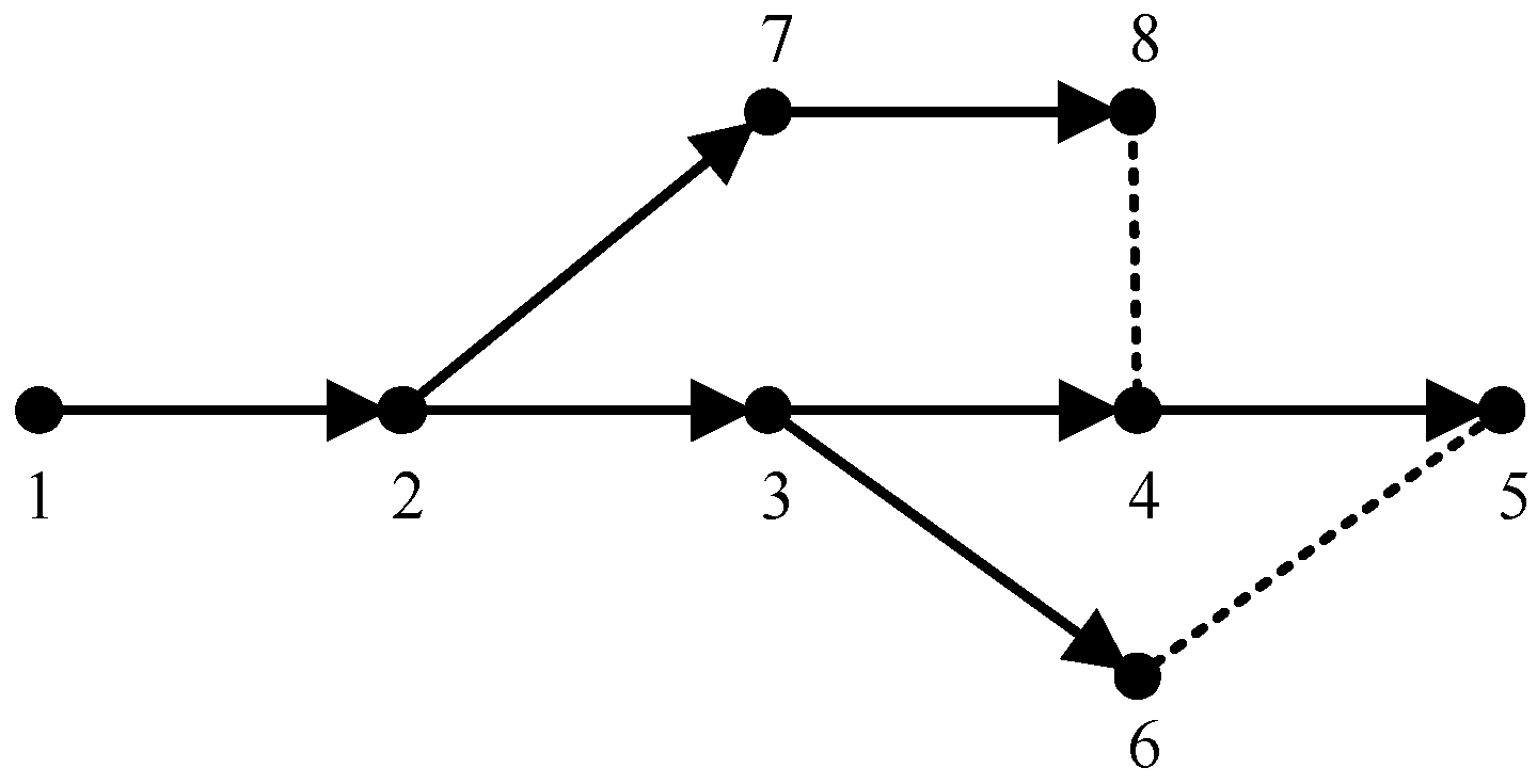
3.1. Nodal Hierarchical Tide Calculation

The general power flow calculation for complex distribution networks is slow, which affects the overall analysis of the distribution network. In this paper, the forward and backward generation method of node layers is used to calculate the power flow, which can not only improve the computational efficiency but also detect the topology structure to determine whether the solution is feasible. According to the branches and nodes of the distribution network, the node association matrix, node layering matrix and upper node matrix must be defined in the distribution system [19].

The node association matrix in the distribution network is defined as follows:

$$N\mathrm{ode}(i,j)=\left\{\begin{array}{l}1 Nodes i,j are associated\\ 0 Nodes i,j are not associated\end{array}\right.,$$

(8)

where i and j are any two nodes in the distribution network.

The node layering matrix is defined as Layer M, where the number of column layers in the matrix and the number of each layer are node numbers.

The upper node matrix is defined as Upper N, which consists of a row with N columns corresponding to the number of nodes in the distribution network. The number in each column is the number of the upper layer node corresponding to the node number in the column.

The node hierarchy is carried out with the radial network of eight nodes shown in Figure 1, with branches 4–8 and 5–6 as contact switches (open). The remaining branches are segment switches (closed).

In normal operation, the contact switch is on while the segment switch is closed. Then, the node association matrix of the network shown in Figure 1 can be described as

$$N\mathrm{ode}(i,j)=\left[\begin{array}{cc}\begin{array}{cc}\begin{array}{ccc}\begin{array}{ccc}\begin{array}{cc}\begin{array}{l}0\\ 1\\ 0\\ 0\\ 0\\ 0\\ 0\\ 0\end{array}& \begin{array}{l}1\\ 0\\ 1\\ 0\\ 0\\ 0\\ 1\\ 0\end{array}\end{array}& \begin{array}{l}0\\ 1\\ 0\\ 1\\ 0\\ 1\\ 0\\ 0\end{array}& \begin{array}{l}0\\ 0\\ 1\\ 0\\ 1\\ 0\\ 0\\ 0\end{array}\end{array}& \begin{array}{l}0\\ 0\\ 0\\ 1\\ 0\\ 0\\ 0\\ 0\end{array}& \begin{array}{l}0\\ 0\\ 1\\ 0\\ 0\\ 0\\ 0\\ 0\end{array}\end{array}& \begin{array}{l}0\\ 1\\ 0\\ 0\\ 0\\ 0\\ 0\\ 1\end{array}\end{array}& \begin{array}{l}0\\ 0\\ 0\\ 0\\ 0\\ 0\\ 1\\ 0\end{array}\end{array}\right],$$

(9)

Since Node(i,j) is a symmetric matrix, the network topology can be determined by the upper triangular matrix Node(i,j)′.

$$N\mathrm{ode}(i,j)\prime =\left[\begin{array}{cc}\begin{array}{cc}\begin{array}{ccc}\begin{array}{ccc}\begin{array}{cc}\begin{array}{l}0\\ 0\\ 0\\ 0\\ 0\\ 0\\ 0\\ 0\end{array}& \begin{array}{l}1\\ 0\\ 0\\ 0\\ 0\\ 0\\ 0\\ 0\end{array}\end{array}& \begin{array}{l}0\\ 1\\ 0\\ 0\\ 0\\ 0\\ 0\\ 0\end{array}& \begin{array}{l}0\\ 0\\ 1\\ 0\\ 0\\ 0\\ 0\\ 0\end{array}\end{array}& \begin{array}{l}0\\ 0\\ 0\\ 1\\ 0\\ 0\\ 0\\ 0\end{array}& \begin{array}{l}0\\ 0\\ 1\\ 0\\ 0\\ 0\\ 0\\ 0\end{array}\end{array}& \begin{array}{l}0\\ 1\\ 0\\ 0\\ 0\\ 0\\ 0\\ 0\end{array}\end{array}& \begin{array}{l}0\\ 0\\ 0\\ 0\\ 0\\ 0\\ 1\\ 0\end{array}\end{array}\right],$$

(10)

Since node 1 is a power node, the search is performed from this node. The element in column 1 and row 1 of the node layering matrix is “1”; that is, Layer M = [1], and the corresponding Upper N = [0 0 0 0 0 0 0 0 0 0].

To find the second layer of nodes: The element of the first column of the upper node hierarchy matrix is “1”, then find the column where the element “1” is in the first row of the upper triangular matrix, which is the second column, so Layer M = [1 2], and the second column of the upper node matrix is “1”, that is, Upper N = [0 1 0 0 0 0 0 0].

And so on, until Upper N, in addition to the first element, is “0”, and the rest is not “0”, which means that the network nodes have been searched. The final node layering matrix and upper node matrix can be derived as follows.

$$Upper N=[0 1 2 3 4 3 2 7],$$

(11)

$$Layer M=\left[\begin{array}{ccc}1& 2& \begin{array}{ccc}3& 4& 5\end{array}\\ 0& 0& \begin{array}{ccc}7& 8& 0\end{array}\\ 0& 0& \begin{array}{ccc}0& 6& 0\end{array}\end{array}\right],$$

(12)

The final Layer M shows the hierarchy of the network, the Upper N shows the upper nodes connected to each node, and the end nodes of the network are 5, 6 and 8. After the hierarchy is completed, the tide is calculated using the traditional forward–back substitution method.

3.2. Coding Strategy

The distribution network usually uses ring structure radial operation; that is, every close contact switch forms a ring network. To meet the structural requirements of distribution network operation, it is necessary to disconnect a segment switch in the ring network to keep the network radial. Since there are many branches in the distribution network, a reasonable strategy for coding the branches must be chosen. To reduce the solution space for reconstructing the distribution network, an integer ring network coding strategy is used to code each branch. The individual steps are as follows:

The entire network switch is closed to form a number of ring networks. The number of ring networks is equal to the number of contact switches.

The switches of the entire network are numbered with natural numbers from small to large. They are classified according to their respective ring networks.

The switches in each ring network are renumbered within the ring. The contact switches in each ring network are numbered last.

In the following, the IEEE 33-bus distribution network shown in Figure 2 is used as an example for the coding explanation, and the coding results are shown in

Table 1. Coding results.

Ring Network	Actual Switch Number	Switch Number
L1	7 6 5 4 3 2 20 19 18 33	1–10
L2	14 13 12 11 10 9 34	1–7
L3	11 10 9 8 7 6 5 4 3 2 21 20 19 18 35	1–15
L4	17 16 15 14 13 12 11 10 9 8 7 6 25 26 27 28 29 30 31 32 36	1–21
L5	24 23 22 28 27 26 25 4 3 37	1–11

[19].

As shown in Figure 1, there are 32 segment switches and 5 contact switches in the network, of which switch 1 is not in any ring network and is therefore not encoded. In this coding strategy, the particle dimension is the number of ring networks, and the specific value of each dimension represents the number of switches that are not connected in the corresponding ring networks. For example, Swarm = [10, 7, 15, 21, 37] disconnects switches 33, 34, 35, 36, 37. Table 1 shows that the upper limit of each particle dimension is U_b = [10, 7, 15, 21, 11], and the lower limit is L_b = [1, 1, 1, 1, 1].

The reconfiguration of the distribution network should correspond to the radial network structure and not form a ring network; that is, an independent ring network is formed when a contact switch is closed and a disconnector is switched off. Therefore, the number of unfeasible solutions will increase in the reconstruction process. To ensure that there are no ring networks and isolated islands in the reconstructed network, the branch loop correlation matrix is introduced and combined with the node layering strategy to determine the infeasible solution. The branch loop correlation matrix T is described as

$$T=\left[\begin{array}{cccc}\begin{array}{cc}\begin{array}{l}{S}_{11}\\ S_{21}\\ S_{31}\\ S_{41}\\ S_{51}\end{array}& \begin{array}{l}{S}_{12}\\ S_{22}\\ S_{32}\\ S_{42}\\ S_{52}\end{array}\end{array}& \begin{array}{l}{S}_{13}\\ S_{23}\\ S_{33}\\ S_{43}\\ S_{53}\end{array}& \begin{array}{l}{S}_{14}\\ S_{24}\\ S_{34}\\ S_{44}\\ S_{54}\end{array}& \begin{array}{l}{S}_{15}\\ S_{25}\\ S_{35}\\ S_{45}\\ S_{55}\end{array}\end{array}\right],$$

(13)

where the rows in matrix T represent the five loops formed by the IEEE 33-node distribution system, and the columns represent the disconnected switch numbers. S = 0 indicates the switch is closed, and S = 1 indicates the switch is disconnected; for example, S₂₃ = 0 indicates the third switch of the second loop is closed.

Judgment rules are as follows:

If the matrix T is a diagonal array after particle iteration, there is no common switch in the loop, and a feasible solution is obtained.

If the matrix T is not diagonal and there are two identical rows, this means that the same switch is interrupted twice, and a loop network is created. That is not a feasible solution.

If the matrix T is not diagonal and does not have the same two rows, then the upper node matrix Upper N is needed to make a judgment. If the first element of Upper N is zero and the remaining elements are non-zero, a feasible solution is obtained. If the first element of Upper N is zero and the remaining elements are non-zero, this indicates that the line is islanded, and a non-feasible solution is obtained.

Take the distribution network IEEE with 33 nodes as an example. If the combinations of the switched-off switches are 33, 34, 35, 36 and 37, the following three matrices can be obtained by coding.

$$T=\left[\begin{array}{cccc}\begin{array}{cc}\begin{array}{l}1\\ 0\\ 0\\ 0\\ 0\end{array}& \begin{array}{l}0\\ 1\\ 0\\ 0\\ 0\end{array}\end{array}& \begin{array}{l}0\\ 0\\ 1\\ 0\\ 0\end{array}& \begin{array}{l}0\\ 0\\ 0\\ 1\\ 0\end{array}& \begin{array}{l}0\\ 0\\ 0\\ 0\\ 1\end{array}\end{array}\right],$$

(14)

$$Layer M=\left[\begin{array}{cccc}\begin{array}{cccc}\begin{array}{cccc}\begin{array}{cccc}\begin{array}{cccc}\begin{array}{ccc}\begin{array}{l}1\\ 0\\ 0\end{array}& \begin{array}{l}2\\ 0\\ 0\end{array}& \begin{array}{l}3\\ 19\\ 0\end{array}\end{array}& \begin{array}{l}4\\ 20\\ 23\end{array}& \begin{array}{l}5\\ 21\\ 24\end{array}& \begin{array}{l}6\\ 22\\ 25\end{array}\end{array}& \begin{array}{l}7\\ 26\\ 0\end{array}& \begin{array}{l}8\\ 27\\ 0\end{array}& \begin{array}{l}9\\ 28\\ 0\end{array}\end{array}& \begin{array}{l}10\\ 29\\ 0\end{array}& \begin{array}{l}11\\ 30\\ 0\end{array}& \begin{array}{l}12\\ 31\\ 0\end{array}\end{array}& \begin{array}{l}13\\ 32\\ 0\end{array}& \begin{array}{l}14\\ 33\\ 0\end{array}& \begin{array}{l}15\\ 0\\ 0\end{array}\end{array}& \begin{array}{l}16\\ 0\\ 0\end{array}& \begin{array}{l}17\\ 0\\ 0\end{array}& \begin{array}{l}18\\ 0\\ 0\end{array}\end{array}\right],$$

(15)

$$\begin{array}{c}Upper N=\left[\begin{array}{cccc}\begin{array}{cccc}\begin{array}{cccc}\begin{array}{cccc}\begin{array}{cccc}\begin{array}{cccc}\begin{array}{cc}0& 1\end{array}& 2& 3& 4\end{array}& 5& 6& 7\end{array}& 8& 9& 10\end{array}& 11& 12& 13\end{array}& 14& 15& 16\end{array}& 17& 2& 19\end{array}\right.\\ \left.\begin{array}{cccc}\begin{array}{cccc}\begin{array}{cccc}\begin{array}{cccc}20& 21& 3& 23\end{array}& 24& 6& 26\end{array}& 27& 28& 29\end{array}& 30& 31& 32\end{array}\right]\end{array},$$

(16)

At this time, the matrix T is a diagonal array, and the matrix Upper N is not zero except for the first element, so there are no islands in the line, and this switching solution is a feasible solution.

4. Chaotic Particle Swarm Chicken Flock Algorithm

4.1. Chaotic Particle Swarm Algorithm

The particle swarm optimization (PSO) algorithm has good local search capability and search efficiency in reconfiguring distribution networks. However, the uncertainty and randomness in the process of initialization and iteration cause the particles to fall into a local optimum. The Logistic equation is introduced in [20]. Based on the diversity and ergodicity of the chaotic search population, the chaotic setting of particle initialization is performed. Chaos disturbs the particles with poor fitness values, which not only prevents the inert particles from falling into the local optimum but also increases the convergence rate of the particles. The specific iterative process of PSO is the following formula:

$$\left\{\begin{array}{l}{v}_{id}^{k+1}=\omega v_{id}^k+c_1{r}_1\left(pbes{t}_{id}-x_{id}^k\right)+c_2{r}_2\left(gbes{t}_{id}-x_{id}^k\right)\hfill \\ x_{id}^{k+1}=x_{id}^k+v_{id}^k\hfill \end{array}\right.,$$

(17)

where ω represents inertia weight, c₁ and c₂ represent acceleration coefficients, r₁ and r₂ are random numbers between [0, 1], pbest and gbest represent individual optimum and global optimum, respectively, and x_id and v_id represent the position and velocity of the kth iteration, respectively.

The logistic equation is formulated as

$$u_{n+1}=\mu u_n\left(1-u_n\right),$$

(18)

where u is the control variable, generally taken as 4, and x_n is taken as a random number in the interval of [0, 1].

The process steps of particle swarm chaos optimization are:

Create a random vector between 0 and 1 in the search space, denoted as u₁.

Iterate m chaotic variables using Equation (17), where m is the step size of the search space (taken as 5 in this paper), and map the chaotic sequence to the search space by Equation (18) to obtain the initial population as follows:

$$x_0=x_{\min }+u_n\left(x_{\max }-x_{\min }\right),$$

(19)

where x_max and x_min represent the upper and lower limits of particle search, respectively.

The chaotic perturbation of the particles is performed using Equation (19), and the magnitude of the fitness value of the particles is calculated.

$$x\prime =round\left(x-ax{u}_n\right),$$

(20)

where α represents the perturbation coefficient, here taken as 2, and x′ and x represent the positions of the particles before and after the perturbation, respectively.

Compare the fitness value of the particle before and after the disturbance. If the fitness value of the particle after the disturbance is better than before the disturbance, the particle is replaced, and vice versa.

4.2. Chicken Swarm Optimization

Chicken Swarm Optimization (CSO) is a novel bionic optimization algorithm that uses the hierarchy and group activity behavior of chickens. The idea is to divide the flock into different groups. The roosters had the strongest search ability and the best fitness scores. The number is equal to the number of groups. The search ability and fitness values of the hens are slightly inferior to those of the roosters. The rest of the hens are considered as chicks. The roosters in each group acted as lead chicks to guide the hens to forage, and the chicks foraged near the corresponding hens, which allowed information exchange between the groups. The roosters, hens and chicks in the group were re-selected for each round of foraging. The steps of the CSO algorithm are as follows:

Initialize the parameters and set the flock size N and the number of different chickens.

Calculate the fitness value of the chickens, divide them into roosters, hens and chicks according to their size, and divide them into different groups to establish the subordination relationship.

Determine if the grouping of the chickens needs to be updated, and if so, update it; otherwise, proceed to the next step.

Update the positions of roosters, hens and chicks and calculate the global optimum value.

Determine if the maximum number of iterations has been reached. If yes, output the result; otherwise, return to the third step.

4.3. Chaotic Particle Swarm Chicken Swarm Fusion Optimization

In order to efficiently use the global and local search capabilities of the CSO algorithm and overcome the disadvantage of small particle search radius in the iterative process, the Chaotic Particle Swarm Chicken Swarm Fusion Optimization (CPSCSFO) algorithm is proposed by combining the CPSO algorithm and CSO algorithm. It is applied to the optimal reconfiguration of distribution networks with DG. The steps of the CPSCSFO algorithm are as follows:

Chaos setting for particle initialization: calculate the fitness value of the particles by Equation (17), classify the particles into X particles, Y particles and Z particles in different proportions according to the size of the fitness value, and group the particles with the number of groups as the number of X particles.

Determine if the population system needs to be reconstructed and, if so, reclassify the particles according to the fitness value; otherwise, proceed to the next step.

Update the position of X particles, and the formula is as follows:

$$X_{i,j}^{t+1}=X_{i,j}^t\left(1+Rand\left(0,{\sigma }^2\right)\right),$$

(21)

$${\sigma }^2=\left\{\begin{array}{l}1,f_i⩽f_k\hfill \\ \exp \left(\left(f_k-f_i\right)/\left(\left|f_i\right|+\epsilon \right)\right),f_i>f_k,r\ne i,r\in [1,RN]\hfill \end{array}\right.,$$

(22)

where Rand(0,σ²) represents Gaussian distribution, and the mean and variance are 0 and sigma, respectively, f_i and f_k represent particle i and particle k objective functions, respectively, and ε is an infinitesimal number.

Update the position of particle Y, and the formula is as follows:

$$X_{i,j}^{t+1}=X_{i,j}^t+s_1{r}_1\left(X_{s_1,j}^t-X_{i,j}^t\right)+s_2{r}_2\left(X_{s_2,j}^t-X_{i,j}^t\right),$$

(23)

$$s_1=\exp \left(\left(f_i-f_{s_1}\right)/\left(\left|f_i\right|+\epsilon \right)\right),$$

(24)

$$s_2=\exp \left(f_{s_2}-f_i\right),$$

(25)

where s₁ and s₂ represent the influence factors, r₁ represents the X particles in the Y particle group, and r₂ represents the Z particles in the Y particles and the particles in the other groups.

Update the position of Z particles, and the formula is as follows:

$$X_{i,j}^{t+1}=X_{i,j}^t+F_{fl}\left(X_{m,j}^t-X_{i,j}^t\right)$$

(26)

where X_g,j represents the position of Z particles corresponding to Y particles in the same group, F_fl is the search parameter, which indicates that Z particles are bounded by Y particles, and take values in [0, 2].

The particles are subjected to chaos perturbation, and the fitness values of the particles before and after perturbation are compared. If the fitness values of the particles after the perturbation are better than those before the perturbation, the fitness values of the particles are updated and vice versa.

4.4. Algorithm Implementation Flow

When the distribution network is reconstructed, the radial network is guaranteed. The particles in the CPSCSFO algorithm are set to the switch combination mode, and the branch loop matrix and hierarchical node strategy are used to determine the infeasible solution. Accurate and efficient calculation of the distribution network under the constraints of combining network switching states with minimum network loss is required. The algorithm flow chart is shown in Figure 3. The calculation steps of the CPSCSFO algorithm in the optimal reconfiguration of the distribution network are as follows:

Step 1: Set the parameters of the CPSCSFO algorithm and define the relevant variables, then read in the distribution network structure data. Initialize the position and velocity of each particle based on the chaotic sequence.

Step 2: Determine if the particles need to reconfigure the hierarchy (the group to redraw the category), and if so, perform Step 3; otherwise, perform Step 4.

Step 3: Create the population hierarchy according to the good and bad fitness values of the population particles, use the rules of the population hierarchy to divide the particles into different groups, and determine the mother–child relationship between particles Y and Z and that particle Y belongs to particle X.

Step 4: Iterative updates are performed according to the X, Y and Z particle location update formulae. It is important to ensure that the structure of the distribution network is radial and free of islands.

Step 5: The optimal value after iteration is iteratively searched for a chaotic quadratic optimum. If a better solution exists, it is replaced, and the individual optimum and the global optimum are updated.

Step 6: Determine if the maximum number of iterations has been reached. If so, terminate the algorithm and output the minimum active loss, the voltage distribution and the most worrying state of the breaker combination after the optimal reconfiguration of the distribution network; otherwise, return to Step 2.

5. Case Simulation and Analysis

In this paper, we apply the CPSCSFO algorithm in the IEEE 33-node distribution system shown in Figure 2 for an arithmetic simulation analysis to verify the effectiveness and superiority of the algorithm. The reference voltage of the system is set to 12.66 kV, the reference power is set to 10 MV·A, the active load is 3.715 MW, and the reactive load is 2.3 Mvar. The system includes 37 segment switches and 5 contact switches, and the specific node parameters are given in reference [21]. In the CPSCSFO algorithm, the population size is 50, with X, Y and Z particles accounting for 40%, 40% and 20%, respectively, c₁ = 0.4, c₂ = 1.6, ω = 1, and the maximum number of iterations is 100.

5.1. Distribution Network Reconfiguration without DG

To verify the feasibility of the CPSCSFO algorithm in distribution network reconfiguration without DG, the CPSCSFO algorithm in this paper is compared with the CSO algorithm in reference [22], and the results and voltage distribution curves before and after reconfiguration are shown in

Table 2. Reconfiguration results of distribution network without DG.

Algorithm	Open Switches	Active Power Loss (kW)	Minimum Nodal Voltage (p.u.)
Pre-reconstruction	33 34 35 36 37	202.6747	0.9131
PSO	6 8 13 31 37	140.4834	0.9381
CSO [22]	7 9 14 32 37	139.5500	0.9378
CPSCSFO	7 9 14 32 37	139.5191	0.9378

and Figure 4.

From Table 2, it can be seen that the optimal switch combination is obtained with the CSO algorithm and the proposed algorithm. The minimum node voltage is increased from 0.9131 p.u. to 0.9378 p.u. by 2.71%. The active network loss of the system before reconfiguration is 202.6747 kW, and the active network loss after reconfiguration by the algorithm in this paper is 139.5191 kW, which is 31.2% lower than before reconfiguration, while the active network loss after reconfiguration by the CSO algorithm is 31.1% lower. In addition, the active power loss obtained by using the CPSCSFO algorithm for distribution network optimization is lower than that obtained by the PSO algorithm, and the minimum node voltage is higher. This shows that the CPSCSFO algorithm has good application value for distribution network optimization and reconfiguration.

Figure 4 shows the voltage distribution of each node in the distribution network before and after reconfiguration. From this, it can be seen that reconfiguration using the CPSCSFO algorithm not only significantly reduces the network loss of the system but also significantly improves the overall voltage distribution.

5.2. Distribution Network Reconfiguration with PQ-Type DG

To verify whether the CPSCSFO algorithm can incorporate a single DG for distribution network reconfiguration, four distributed power sources of PQ type are used for simulation in this paper, and the specific access locations and network connection parameters are listed in

Table 3. Grid connection parameters of DG [23].

DG Number	1	2	3	4
Location	32	23	17	27
Capacity	50	100	200	100
Power factor	0.9	0.9	0.9	0.9

. The active network loss is used as the objective function and compared with the CS-PSO algorithm of reference [23]. The results before and after reconfiguration are shown in

Table 4. Reconfiguration results of distribution network with PQ-Type DG.

Algorithm	Open Switches	Active Power Loss (kW)	Minimum Nodal Voltage (p.u)
Pre-reconstruction	33 34 35 36 37	148.1182	0.9269
PSO	7 9 14 32 37	117.3438	0.3912
APSO	7 8 14 17 37	114.5495	0.9414
CS-PSO [23]	7 9 14 32 28	113.2365	0.9433
CPSCSFO	7 9 14 31 37	104.5069	0.9488

.

From Table 4, when a single distributed power source is added, the active power loss of the system is reduced from 202.6747 kW to 148.1182 kW, which is 26.92% lower than the original active loss of the network. In addition, the minimum node voltage was increased from 0.9131 p.u. to 0.9269 p.u. Thus, the system access to a single distributed power source not only reduces the active network loss of the system but also results in some improvement in the node voltage. The active power loss after reconfiguration with the algorithm CS-PSO is reduced by 23.55% compared to that before reconfiguration, and the minimum node voltage is improved by 1.74%. The active network loss after reconfiguration with the algorithm in this paper is 104.5069 kW, which is 29.44% lower than that before reconfiguration, and the minimum node voltage is improved from 0.9269 p.u. to 0.9488 p.u., which is 2.31% higher. In addition, compared with the PSO and APSO algorithms, the proposed algorithm has been greatly improved in terms of active network loss and voltage offset. The proposed algorithm can effectively complete the distribution network reconfiguration with PQ-type DG, and its performance has been significantly improved.

As shown in Figure 5, from the voltage distribution before and after reconfiguration with a single DG, it can be seen that the voltage distribution before and after adding PQ-type DG reconfiguration shows an overall increasing trend, while the overall voltage level is better compared to the results of the CS-PSO algorithm. The effectiveness of the algorithm in this paper is demonstrated, and the performance of the system is significantly improved.

From Figure 6, although the convergence speed of the PSO and APSO algorithms is faster than that of the algorithm in this paper, it easily falls into the local optimum, it is difficult to find the global optimum, and it is computationally inefficient. The algorithm proposed in this paper not only finds the optimum faster than the CS-PSO algorithm but also converges faster.

5.3. Distribution Network Reconfiguration with Multiple DGs

To verify whether the CPSCSFO algorithm can connect a variety of DGs for distribution network reconfiguration, four different types of distributed DGs are used for simulation in this paper. Figure 7 shows the location of DG access. The DGs are connected to the network with the parameters listed in

Table 5. Grid connection parameters of DG [24].

DG	Double-Fed Fan	Gas Turbine	Photovoltaic Cell	Wind Asynchronous Generator
Location	30	25	17	4
Capacity	PQ	PV	PI	PQ(V)
Power factor	P = 200 kW	P = 300 kW	P = 300 kW	P = 300 kW
	cos φ = 0.9	Vs = 0.98 p.u.	Is = 50 A

.

The active power loss is used as the objective function and compared with the HDQPSO algorithm in reference [24]. The results before and after reconfiguration are shown in

Table 6. Reconfiguration results of distribution network with Multiple DGs.

Algorithm	Open Switches	Active Power Loss (kW)	Minimum Nodal Voltage (p.u.)
Pre-reconstruction	33 34 35 36 37	108.0021	0.9355
PSO	7 10 14 32 25	101.4236	0.9397
APSO	7 10 14 36 37	101.4155	0.9401
HDQPSO [24]	7 9 14 28 32	85.3985	0.9473
CPSCSFO	9 14 16 28 32	61.6250	0.9688

. When multiple DG sources are added, the active network loss of the system is reduced by 46.71% compared to the initial network, and the minimum node voltage is improved by 2.45%. The active network loss after reconfiguration with the HDQPSO algorithm is reduced by 49.96% compared to the pre-configuration, and the minimum node voltage is improved by 1.25%. The active power loss after reconfiguration with the algorithm in this paper is 61.625 kW, which is 69.59% lower than before reconfiguration, and the minimum node voltage is increased from 0.9355 p.u. to 0.9688 p.u., which is 3.44% higher. This shows that the active power loss is significantly reduced, and the minimum node voltage is significantly increased after reconfiguration. The active power loss and node voltage obtained after reconfiguration with the CPSCSFO algorithm have certain advantages compared to the HDQPSO algorithm. It can be seen from the simulation results that, compared with PSO and APSO algorithms, after adding multiple DGs, the active power loss of the distribution network is greatly reduced, and the voltage level of each node is also improved. After reconfiguration, the node voltage level is significantly increased, and the active power network loss is reduced.

In Figure 8, the voltage distribution curves before and after reconfiguration with multiple DGs are shown, and it can be seen that the voltage levels before and after reconfiguration with multiple DGs are significantly improved, which confirms the high efficiency of the algorithm in this paper. The fitting curves are shown in Figure 9. Compared with the other three algorithms, the algorithm proposed in this paper is the first to achieve convergence, and the convergence accuracy is higher, indicating that the algorithm proposed in this paper can greatly improve the optimization efficiency, improve the overall voltage level of the distribution network, and reduce the system loss when the distribution network is reconfigured with multiple DGs.

The simulation results in three different cases show that the CPSCSFO algorithm used in this paper is not only suitable for the optimal reconstruction of both active and passive structured distribution networks but is also effective in improving the voltage level and reducing the network losses of the distribution network, which can effectively improve the operating cost of the network.

6. Conclusions

In this paper, we present a multi-objective model for optimal reconfiguration of distribution networks using DG with minimum active loss and minimum voltage deviation. The integrated objective function is normalized by adjusting the inertia weights. The CPSCSFO algorithm is applied to the distribution network of the IEEE33 system, which contains DG with different structures, by using the branching loop matrix with a node stratification strategy to determine infeasible solutions. The experimental results show that this solves the distribution network reconfiguration problem.

The node hierarchical forward generation method computes the tide and improves the computational efficiency by avoiding the emergence of ring networks and island solutions during the reconfiguration process through the infeasible solution determination strategy.

The algorithm effectively reduces the active network losses of the system and improves the voltage level of the distribution network nodes, which ensures the quality of the power supply and the operational reliability of the network.

The proposed distribution network optimization reconfiguration algorithm not only improves the efficiency and search ability of the traditional algorithm but also has higher convergence accuracy. It provides a reference value for the future development of the distribution network.

References

1. Shukla, J.; Das, B.; Pant, V. Stability constrained optimal distribution system reconfiguration considering uncertainties in correlated loads and distributed generations. Int. J. Elect. Power Energy Syst. 2018, 99, 121–133. [Google Scholar] [CrossRef]
2. Ali, M.H.; Kamel, S.; Hassan, M.H.; Tostado-Veliz, M.; Zawbaa, H.M. An improved wild horse optimization algorithm for reliability based optimal DG planning of radial distribution networks. Energy Rep. 2022, 8, 582–604. [Google Scholar] [CrossRef]
3. Cupelli, L.; Cupelli, M.; Ponci, F.; Monti, A. Data-Driven Adaptive Control for Distributed Energy Resources. IEEE Trans. Sustain. Energy 2019, 10, 1575–1584. [Google Scholar] [CrossRef]
4. Yazdanian, M.; Mehrizi-Sani, A. Distributed Control Techniques in Microgrids. IEEE Trans. Smart Grid. 2014, 5, 2901–2909. [Google Scholar] [CrossRef]
5. Blaabjerg, F.; Yang, Y.H.; Yang, D.S.; Wang, X.F. Distributed Power-Generation Systems and Protection. Proc. IEEE 2017, 105, 1311–1331. [Google Scholar] [CrossRef]
6. Gerez, C.; Silva, L.I.; Belati, E.A.; Sguarezi Filho, A.J.; Costa, E.C.M. Distribution network reconfiguration using selective firefly algorithm and a load flow analysis criterion for reducing the search space. IEEE Access 2019, 7, 67874–67888. [Google Scholar] [CrossRef]
7. Samman, M.A.; Mokhlis, H.; Mansor, N.N.; Mohamad, H.; Suyono, H.; Sapari, N.M. Fast optimal network reconfiguration with guided initialization based on a simplified network approach. IEEE Access 2020, 8, 11948–11963. [Google Scholar] [CrossRef]
8. Khodr, H.M.; Martinez-Crespo, J.; Matos, M.A.; Pereria, J. Distribution systems reconfiguration based on OPF using benders decomposition. IEEE Trans. Power Deliv. 2009, 24, 2166–2176. [Google Scholar] [CrossRef]
9. Jabr, R.A.; Singh, R.; Pal, B.C. Minimum loss network reconfiguration using mixed-integer convex programming. IEEE Trans. Power Syst. 2012, 27, 1106–1115. [Google Scholar] [CrossRef]
10. Zin, A.A.M.; Ferdavani, A.K.; Bin Khairuddin, A.; Naeini, M.M. Two circular-updating hybrid heuristic methods for minimum-loss reconfiguration of electrical distribution network. IEEE Trans Power Syst. 2013, 28, 1318–1323. [Google Scholar]
11. Chen, K.; Pan, L. Design of distribution network reconfiguration containing distributed generation based on GA-QPSO algorithm. Res. Explor. Lab. 2022, 41, 111–115. [Google Scholar]
12. Xu, X.Q.; Wang, B.; Zhao, H.S.; Du, Z.; Yang, D.J.; Liu, J.; Liu, Y.G.; Hu, P. Reconfiguration of two-voltage distribution network based on cuckoo search and simulated annealing algorithm. Power Syst. Prot. Control 2022, 48, 84–91. [Google Scholar]
13. Wang, L.M.; Cheng, J.; Wang, W.Q. Research on distribution network reconfiguration with distributed generation based on improved grey wolf optimizer. Mod. Electr. Power 2022, 39, 56–63. [Google Scholar]
14. Li, C.; Qin, L.J.; Duan, H. Research on reconfiguration of distribution network with photovoltaic generation based on improved group search optimizer. Acta Energy Sol. Sin. 2022, 43, 213–218. [Google Scholar]
15. Shaheen, A.M.; Elsayed, A.M.; Ginidi, A.R.; El-Sehiemy, R.A.; Elattar, E.E. Improved Heap-Based Optimizer for DG Allocation in Reconfigured Radial Feeder Distribution Systems. IEEE Syst. J. 2022, 16, 6371–6380. [Google Scholar] [CrossRef]
16. Shaheen, A.M.; El-Sehiemy, R.A.; Kamel, S.; Elattar, E.E.; Elsayed, A.M. Improving Distribution Networks’ Consistency by Optimal Distribution System Reconfiguration and Distributed Generations. IEEE Access 2021, 9, 67186–67200. [Google Scholar] [CrossRef]
17. Shaheen, A.M.; Elsayed, A.M.; Ginidi, A.R.; El-Sehiemy, R.A.; Elattar, E.E. Reconfiguration of electrical distribution network-based DG and capacitors allocations using artificial ecosystem optimizer: Practical case study. Alex. Eng. J. 2021, 61, 6105–6118. [Google Scholar] [CrossRef]
18. Shaheen, A.M.; Elsayed, A.M.; Ginidi, A.R.; El-Sehiemy, R.A.; Elattar, E.E. A heap-based algorithm with deeper exploitative feature for optimal allocations of distributed generations with feeder reconfiguration in power distribution networks. Knowl. Based Syst. 2022, 6, 241. [Google Scholar] [CrossRef]
19. Liu, D.; Zhang, Q.; Lv, G.Y. Improvement and application of quantum-behaved particle swarm optimization in distribution network reconfiguration. Electr. Meas. Instrum. 2022, 59, 58–65. [Google Scholar]
20. Xu, X.B.; Zheng, K.F.; Li, D.; Wu, B.; Yang, Y.X. New chaos-particle swarm optimization algorithm. J. Commun. 2012, 33, 24–30. [Google Scholar]
21. Gong, Y.J.; Li, J.J.; Zhou, Y.; Yun, L.; Chung, S.H.; Shi, Y.H.; Zhang, J. Genetic Learning Particle Swarm Optimization. IEEE Trans. Cybern. 2017, 46, 2277–2290. [Google Scholar] [CrossRef] [PubMed]
22. Wang, X.C.; Hu, H.M.; Liu, L. Distribution network reconfiguration based on chicken swarm optimization algorithm. Electrotech. Electr. 2016, 219, 20–24. [Google Scholar]
23. Xu, Y. Application of improved particle swarm optimization in distribution network reconfiguration with distributed generation. Electr. Meas. Instrum. 2021, 58, 98–104. [Google Scholar]
24. Xu, L.Z. Research on Distribution Network Reconfiguration Containing Distributed Generation. Master’s Thesis, Nanchang Hangkong University, Nanchang, China, 2017. [Google Scholar]
Figure 1. Radial network of 8 buses.
Energies 16 07185 g001
Figure 2. IEEE 33-node distribution system.
Energies 16 07185 g002
Figure 3. Flowchart of CPSCSFO algorithm.
Energies 16 07185 g003
Figure 4. Voltage distribution after reconfiguration without DG.
Energies 16 07185 g004
Figure 5. Voltage distribution after reconfiguration with PQ-type DG.
Energies 16 07185 g005
Figure 6. Fitness value curve of distribution network with PQ-Type DG.
Energies 16 07185 g006
Figure 7. Simplified diagram of the IEEE 33-bus distribution network.
Energies 16 07185 g007
Figure 8. Voltage distribution after reconfiguration with multiple DGs.
Energies 16 07185 g008
Figure 9. Fitness value curve of distribution network with Multiple DGs.
Energies 16 07185 g009