Electric Vehicle Fleet Management for a Prosumer Building with Renewable Generation

Abstract

The integration of renewable energy systems in buildings leads to a reduction in energy bills for end users and a reduction in the carbon footprint of such buildings, usually referred to as prosumers. In addition, the installation of charging points for the electric vehicles of people working or living in these buildings can further improve the energy efficiency of the whole system if innovative technologies, such as vehicle-to-building (V2B) technologies, are implemented. The aim of this paper is to present an Energy Management System (EMS) based on mathematical programming that has been developed to optimally manage a prosumer building equipped with photovoltaics, a micro wind turbine and several charging points for electric vehicles. Capabilities curves of renewable power plant inverters are modelled within the EMS, as well as the possibility to apply power curtailment and V2B. The use of V2B technology reduces the amount of electricity purchased from the public grid, while the use of smart inverters for the power plants allows zero reactive power to be drawn from the grid. Levelized cost of electricity (LCOE) is used to quantify curtailment costs, while penalties on reactive power absorption from the distribution network are evaluated in accordance with the current regulatory framework. Specifically, the model is applied to a prosumer building owned by the postal service in a large city in Italy. The paper reports the main results of the study and proposes a sensitivity analysis on the number of charging stations and vehicles, as well as on the consideration of different typical days characterized by different load and generation profiles. This paper also investigates how errors in forecasting energy production from renewable sources impact the optimal operation of the whole system.

1. Introduction

The building sector is a major consumer of energy, accounting for approximately 40% of final energy consumption and 36% of Greenhouse Gas (GHG) emissions in the European Union (EU). Specifically, the electricity consumption constitutes 35% of the energy use in buildings [1,2].

To address this issue, governments have implemented various measures in recent years to reduce energy consumption in buildings and promote the adoption of Renewable Energy Sources (RESs). The European Commission has introduced the so-called “Fit for 55” package, which aims to reduce GHG emissions by at least 55% by 2030 (compared to 1990 levels) and increase the market share of renewable energy by up to 40%. Specifically, within the building sector, the target is to achieve a 49% share of RES energy consumption [3].

In addition, private transportation accounts for 15% of CO₂ emissions in the EU. The “Fit for 55” package proposes a gradual reduction plan for CO₂ emissions from private vehicles, with a goal of achieving a 100% reduction by 2035. This implies that all new cars and vans entering the market after 2035 should be zero-emission vehicles, leading to reduced pollution and improved air quality, especially in densely populated areas [3]. National governments will play a crucial role in this transition by promoting the adoption of Electric Vehicles (EVs) and RESs, starting with public facilities and buildings such as schools, universities, and government offices [4].

RES technologies will play a leading role in boosting this transition: in particular, in dealing with the building sector, small-scale applications of RESs will be needed. The most suitable technologies for this application are Photovoltaic (PV) units and Wind Turbines (WTs). PV units are one of the major sources of distributed renewable energy and are usually involved in domestic rooftop installations, allowing the exploitation of previously unused spaces [5]. This trend is favoured due to the continuous decrease in PV installation prices and the incentives issued by governments.

Small-size WTs are typically positioned in close proximity to facilities in order to minimize potential wind disturbances caused by buildings but can also be installed on the rooftops of high-rise buildings to exploit the high wind speed. In urban areas, wind speed estimation is very important in order to evaluate the suitability of WT installation [6].

However, due to their inherent unpredictability, RESs are unable to instantly follow the profile of the demand. In order to cope with the imbalance between generation and load, Energy Storage Systems (ESSs) such as Battery Energy Storage Systems (BESSs) are commonly installed, enhancing the flexibility of the system. Anyway, in smaller-scale applications such as buildings, the integration of BESSs can significantly impact both installation and operational costs.

Within this regulatory and technical framework, so-called “Prosumption” is gaining increasing importance. “Prosumption” is the combination of both the consumption and the production of energy, and those who are involved in these activities are called “Prosumers”. In addition to consuming their own renewable energy surplus, users have the option to sell it to the external power grid and receive compensation from the market operator. Prosumers are simultaneously consumers, producers and sellers of renewable energy [7].

Small-scale prosumers are residential facilities with PV units and BESS or PV units and EVs. Larger-scale applications of prosumption are represented by public institutions and small/medium enterprises that may exploit larger-size facilities, like larger PV units, WTs and BESSs and a fleet of EVs.

Besides the economic advantage deriving from the sale of surplus electricity to the external network, other forms of revenue may come from the provision of ancillary balancing services to the distribution system operator, like Frequency Containment Reserve (FCR) and automatic Frequency Restoration Reserve (aFRR), well suited for integrated PV-battery prosumers, as shown in [8] and references therein. Prosumers also offer distributed energy capacity, as highlighted in [9].

RESs are exploited not only to generate active power but also to satisfy the reactive power request of the load, thanks to the reactive power exchange capability of the inverters; in addition, by adjusting their reactive power injection/absorption, they provide voltage regulation at the node at which they are connected, even during night [10,11].

EVs are progressively substituting traditional combustion engine vehicles. In order to fully exploit the advantage of this technology, EVs can be connected to buildings, enabling the so-called Vehicle-to-Building (V2B) functionality: in this application, EVs do not behave only like a load but, when in idle mode, their battery can provide power to the building or absorb surplus power from the building, thanks to the bidirectionality of the power flow. V2B represents an alternative to non-mobile BESSs, also in Local Energy Communities (LECs) [12].

V2B applications have several positive effects on the vehicle–building system: they contribute to the dumping of the oscillation and unpredictability of the production of RESs [13], allowing the time shifting of energy and increasing the level of RES self-consumption for the user [14]; peak shaving is possible with V2B, reducing the grid peak generation power [15]. In addition, EVs can be used as a backup source in case of power outages [16]. Moreover, acting as storage systems, they can be used to reduce RES curtailment [17] and to supply energy to buildings in residential districts [18] where they stay parked for a long time. Enabling V2B technologies for EV fleets opens the door for the participation of EVs in primary frequency regulation, acting as spinning resources that are able to comply with national grid codes in terms of effectiveness and promptness [17,18].

The complexity of a system composed of a building and one or several EVs, with the possibility of performing V2B, means that an Energy Management System (EMS) is required in order to optimize the power flows between all the units.

Several examples of EMS applied to V2B can be found in the literature. In [19], a building EMS is proposed in order to integrate EVs with the aim of levelling the peak load demand to the off-peak hours. In [20] and in therein references, several EMSs and advanced control strategies are proposed, focusing in particular on the integration of buildings and EVs. In [21], the authors focus on optimal strategies for the smart charging of EVs in facilities that couple unpredictable RESs and infrastructure for electric mobility, while in [22], the authors investigated how the number of EVs in commercial buildings impacts electricity bills and how they can act as storage systems in buildings operating in the island mode. In [23], the proposed control strategy is designed to enable the effective interaction of a PV system, stationary batteries, and an EV within a prosumer installation. Assuming that the storage system works according to a fixed charging and discharging schedule, the proposed algorithm controls the operation of the EV battery, taking into account trip data introduced by the driver in order for the EV battery to reach the planned level of state of charge before the time of driving. In [24], the authors propose heuristic vehicle-to-home charging strategies with the goal of increasing self-sufficiency, vehicle availability and traction battery lifetime in different scenarios characterized by different EV driver behaviours. An EMS designed to optimize demand response in a prosumer building is described in [25], where the EV fleet is modelled considering stochastic characteristics, and PV production is modelled under uncertainty using actual data collected via smart meters. In [26], an EMS designed for the microgrids of building prosumers is described, considering both active and reactive power exchange.

An EMS for a public building with RES generation from PV and WT units and an EV for mail delivery is proposed in [27]. The present paper represents an extension of the model proposed in [27]. The main objective of this paper is to define an EMS that ensures the optimal operation and scheduling of a postal service-owned building located in a large city in Italy. The building is connected to the medium-voltage distribution network and is also fed by two small-size RES units: a PV unit and a WT unit; it acts like a prosumer of electricity, thanks to the bidirectional connection to the network. Several Electric Delivery Vehicles (EDVs) are allocated to the facility for mail transportation; each vehicle has a dedicated charging station. Innovative aspects of the model are represented through the modelling of the capability curves of the RES inverters within the EMS to optimally manage reactive power flows, as well as via the introduction of costs related to RES curtailment and reactive power absorption in the objective function. By running the EMS over an entire year with an hourly time resolution, the study aims to evaluate the impact of the number of EVs on the operation of the building, both from an energy and an economic point of view. Three scenarios are analysed, considering the number of EDVs equal to 10, 50 and 100. A sensitivity analysis is developed by varying the price of sale and purchase of electricity, as well as the number of Equivalent Operating Hours (EOHs) of the renewable power plants.

This paper is structured as follows: Section 2 describes the whole system, providing essential data and assumptions that have been made by the authors, and presents a comprehensive description of the optimization mathematical model that has been set up. Section 3 shows the results of the study and discusses them by comparing the three scenarios. Some concluding remarks, together with a discussion of potential future developments, are provided in Section 4.

2. Materials and Methods

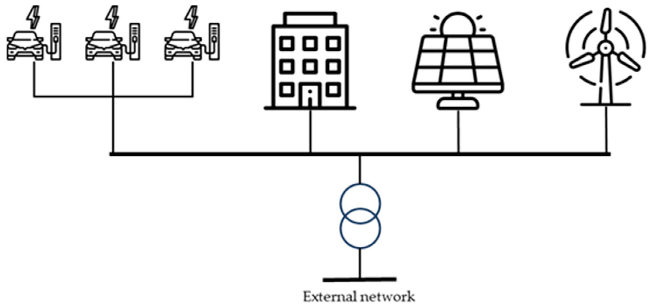
2.1. System Description and Input Data

The developed mathematical model is an EMS, which makes it possible to apply optimal management strategies to the daily operation of a prosumer building equipped with renewable energy systems (mainly PV and WTs) and charging points for EVs. RES power plants are connected to the AC network through smart inverters able to manage both active and reactive powers, while EV charging stations are of the V2B type. As shown in Figure 1, the whole system is modelled as a microgrid connected to the medium-voltage distribution network, and each EV has a dedicated charging station. The EMS is based on a Mixed-Integer Linear Programming (MILP) model, having a time horizon consisting of T time intervals (t = 1 … T), each one with a duration equal to Δ.

The main input data of the model are:

• The number of RES power plants, indicated by J;
• The number of EVS, which coincides with the number of charging points, denoted as N;
• The size $A_j^{RES}$ [kVA] of the inverter associated with the j-th RES plant;
• The estimated average power $P_j^{RES,av}$ [kW] that can be generated by the j-th RES plant at time t;
• the curtailment cost $c_j^{RES,curt}$ [EUR/kWh] of the j-th RES plant, represented by its Levelized Cost of Electricity (LCOE);
• The rated capacity $C_n^{EV}$ [kWh] of the battery installed inside the n-th EV, together with its minimum state of charge ${SOC}_n^{EV,min}$ [%];
• The average energy consumption $F_n^{EV}$ [kWh/km] of the n-th EV;
• The transportation demand $D_{n,t}^{EV}$ of the n-th EV in the time interval t, measured in [km];
• Information on the presence of the vehicles at the facility, as expressed by the factor $y_{n,t}^{EV}$, which is equal to 1 when the n-th EV can be connected to its charging point and equal to 0 when the vehicle is not present;
• The minimum power $P_n^{EV,ch,min}$ [kW] that can be delivered to the n-th EV;
• The maximum power $P_n^{EV,ch,max}$ [kW] that can be delivered to the n-th EV;
• The minimum power $P_n^{EV,dch,min}$ [kW] that can be supplied by the n-th EV when it is operated in V2B mode;
• The maximum power $P_n^{EV,dch,max}$ [kW] that can be supplied by the n-th EV when it is operated in V2B mode;
• The charging (${\eta }^{EV,ch})$ and discharging (${\eta }^{EV,dch})$ efficiencies of EVs;
• The electrical load profiles of the building, in terms of active ($P_t^L$) [kW] and inductive reactive power ($Q_t^L$) [kVAr];
• The size $A_{ }^{grid}$ [kVA] of the transformer which connects the microgrid to the medium voltage distribution network;
• The active energy purchase and selling prices, respectively, $p_t^{grid}$ [EUR/kWh] and $r_t^{grid}$ [EUR/kWh];
• The penalty $q_t^{grid}$ [EUR/kVArh] on reactive energy absorbed from the distribution network, as set by the authority.

It is assumed that every RES power plant can exchange both active and reactive power in accordance with its capability curve, which is characterized by the shape of a semi-circle in the first two quadrants of the plane, with the reactive power on the horizontal axis and the active power on the vertical axis. Charging points for EVs work at a unitary power factor. Reactive power can be exchanged by the microgrid with the distribution network, thus enabling the transformer to operate in the four quadrants of the reactive/active power plane. The building does not present manageable loads apart from the EV charging points, whose scheduling can be optimized via the EMS. As further described in Section 2.2, the main goal of the EMS is that of managing RES power plants and EV charging points in order to minimize global Net Costs (NCs) and reduce the curtailment of RES sources. Among the costs, one is represented by the penalties related to the reactive power absorbed from the distribution network; to minimize this term, the role of inverters of RES plants in providing inductive reactive power is investigated.

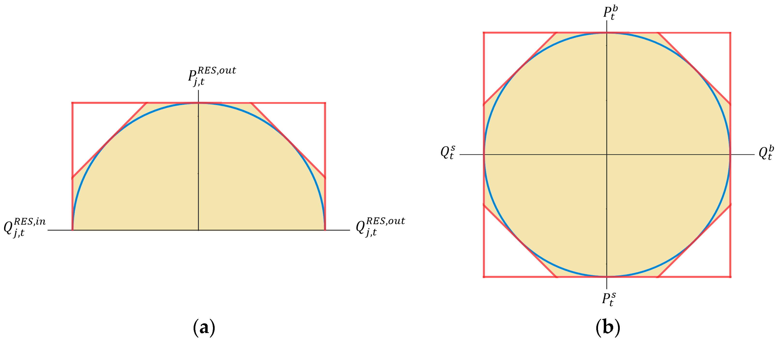
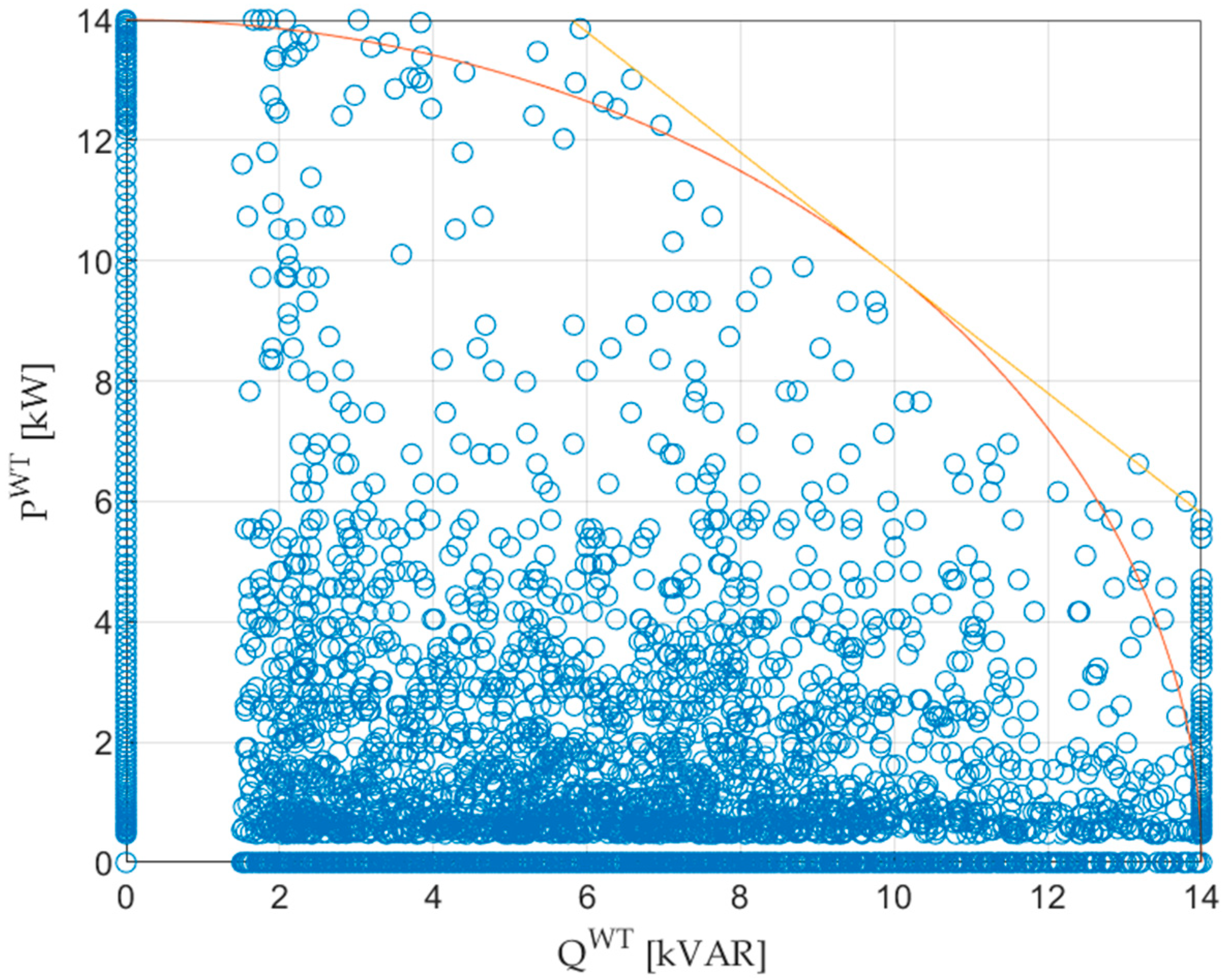
2.2. Mathematical Model

In the mathematical model, RES power plants, EV charging points and the transformer are modelled by a set of linear constraints given by equalities or inequalities correlating with the decision variables, both integer and continuous.

The main decision variables that refer to the operation of j-th RES power plant at time t are:

• $P_{j,t}^{RES,out}$ [kW]: generated active power;
• $P_{j,t}^{RES,curt}$ [kW]: curtailed active power;
• $Q_{j,t}^{RES,in}$ [kVAr]: inductive reactive power absorbed from the microgrid;
• $Q_{j,t}^{RES,out}$ [kVAr]: inductive reactive power supplied to the microgrid.

The relative constraints are defined from (1) to (2). The energy balances (1) set that the active power available from each RES plant is given by the sum between the generated power and the curtailed one, while constraints (2) guarantee that the maximum curtailed power is the available one. Constraints from (3) to (7) are defined to linearize the circular capability curve of inverters in the active power/reactive power plane, as shown in Figure 2a. The operating points lay in the ochre-colored area. In particular, constraints (3) and (4) fix the upper bounds of the inductive reactive power (absorbed and supplied) as a function of the rated apparent power $A_j^{RES}$, whereas constraints (6) and (7) represent the two tangents to the capability curve, respectively, in the first and in the second quadrants at the points of coordinates ($\frac{\sqrt{2}}{2}·A_j^{RES}, \frac{\sqrt{2}}{2}·A_j^{RES})$ and ($-\frac{\sqrt{2}}{2}·A_j^{RES}, \frac{\sqrt{2}}{2}·A_j^{RES})$. The set of binary variables $y_{j,t}^{RES,in}$ and $y_{j,t}^{RES,out}$ is introduced to avoid the simultaneous absorption and supply of inductive reactive power at time t, as ensured by constraints (5).

$$P_{j,t}^{RES,av}-P_{j,t}^{RES,out}-P_{j,t}^{RES,curt}=0\hspace{1em}\hspace{1em}\forall j=1\dots J, \forall t=1\dots T$$

(1)

$$0\le P_{j,t}^{RES,curt}\le P_{j,t}^{RES,av}\hspace{1em}\hspace{1em}\forall j=1\dots J, \forall t=1\dots T$$

(2)

$$0\le Q_{j,t}^{RES,in}\le A_j^{RES}·y_{j,t}^{RES,in}\hspace{1em}\hspace{1em}\forall j=1\dots J, \forall t=1\dots T$$

(3)

$$0\le Q_{j,t}^{RES,out}\le A_j^{RES}·y_{j,t}^{RES,out}\hspace{1em}\hspace{1em}\forall j=1\dots J, \forall t=1\dots T$$

(4)

$$y_{j,t}^{RES,in}+y_{j,t}^{RES,out}\le 1\hspace{1em}\hspace{1em}\forall j=1\dots J, \forall t=1\dots T$$

(5)

$$P_{j,t}^{RES,out}\le -Q_{j,t}^{RES,out}+\sqrt{2}·A_j^{RES}\hspace{1em}\hspace{1em}\forall j=1\dots J, \forall t=1\dots T$$

(6)

$$P_{j,t}^{RES,out}\le -Q_{j,t}^{RES,in}+\sqrt{2}·A_j^{RES}\hspace{1em}\hspace{1em}\forall j=1\dots J, \forall t=1\dots T$$

(7)

The decision variables that describe the active and reactive power exchanged between the microgrid and the distribution network at time t are:

• $P_t^b$ [kW]: active power withdrawn from the distribution network;
• $P_t^s$ [kW]: active power injected into the distribution network;
• $Q_t^b$ [kVAr]: inductive reactive power absorbed from the distribution network.
• $Q_t^s$ [kVAr]: inductive reactive power provided to the distribution network.

Moreover, a set of auxiliary binary variables are needed to avoid the simultaneous absorption and injection of power from/into the distribution network. Specifically, $x_t^b$ and $x_t^s$ are used for active power, while $y_t^b$ and $y_t^s$ for reactive power. The constraints from (8) to (17) model the interaction between the microgrid and the distribution network and are based on the linearization of the transformer capability curve, as reported in Figure 2b. In particular, constraints (8) and (9) limit the maximum active power that can be exchanged, while constraints (11) and (12) do the same for the reactive power. Constraints (10) and (13) ensure the non-simultaneity between absorptions and withdrawals, while constraints (14) to (17) define the limits imposed by the four oblique segments reported in Figure 2b.

$$0\le P_t^b\le A^{grid}·x_t^b\hspace{1em}\hspace{1em}\forall t=1\dots T$$

(8)

$$0\le P_t^s\le A^{grid}·x_t^s\hspace{1em}\hspace{1em}\forall t=1\dots T$$

(9)

$$x_t^b+x_t^s\le 1\hspace{1em}\hspace{1em}\forall t=1\dots T$$

(10)

$$0\le Q_t^b\le A^{grid}·y_t^b\hspace{1em}\hspace{1em}\forall t=1\dots T$$

(11)

$$0\le Q_t^s\le A^{grid}·y_t^s\hspace{1em}\hspace{1em}\forall t=1\dots T$$

(12)

$$y_t^b+y_t^s\le 1\hspace{1em}\hspace{1em}\forall t=1\dots T$$

(13)

$$P_t^b\le -Q_t^b+\sqrt{2}·A^{grid}\hspace{1em}\hspace{1em}\forall t=1\dots T$$

(14)

$$P_t^b\le -Q_t^s+\sqrt{2}·A^{grid}\hspace{1em}\hspace{1em}\forall t=1\dots T$$

(15)

$$P_t^s\le -Q_t^b+\sqrt{2}·A^{grid}\hspace{1em}\hspace{1em}\forall t=1\dots T$$

(16)

$$P_t^s\le -Q_t^s+\sqrt{2}·A^{grid}\hspace{1em}\hspace{1em}\forall t=1\dots T$$

(17)

As far as electric mobility is concerned, the decision variables that refer to the operation of EV charging stations at time t are:

• $P_{n,t}^{EV,ch}$ [kW]: active power supplied to the n-th EV;
• $P_{n,t}^{EV,dch}$ [kW]: active power provided by the n-th EV when operated in V2B mode;
• $E_{n,t}^{EV}$ [kWh]: energy content of the battery in the n-th EV.

The constraints on $P_{n,t}^{EV,ch}$ and $P_{n,t}^{EV,dch}$ can be defined as follows:

$$P_{n,t}^{EV,ch}\ge P_n^{EV,ch,min}·x_{n,t}^{EV,ch} \forall n=1\dots N, \forall t=1\dots T$$

(18)

$$P_{n,t}^{EV,ch}\le P_n^{EV,ch,max}·x_{n,t}^{EV,ch} \forall n=1\dots N, \forall t=1\dots T$$

(19)

$$P_{n,t}^{EV,dch}\ge P_n^{EV,dch,min}·x_{n,t}^{EV,dch}\hspace{1em}\hspace{1em}\forall n=1\dots N, \forall t=1\dots T$$

(20)

$$P_{n,t}^{EV,dch}\le P_n^{EV,dch,max}·x_{n,t}^{EV,dch}\hspace{1em}\hspace{1em}\forall n=1\dots N, \forall t=1\dots T$$

(21)

where the binary variables $x_{n,t}^{EV,ch}$ and $x_{n,t}^{EV,dch}$ become equal to 1 when the n-th vehicle is charging or discharging at time t, respectively. Obviously, as defined in (22), each vehicle can be charged or discharged only when present at the facility ($y_{n,t}^{EV}$ = 1).

$$x_{n,t}^{EV,ch}+x_{n,t}^{EV,dch}\le y_{n,t}^{EV}\hspace{1em}\hspace{1em}\forall n=1\dots N, \forall t=1\dots T$$

(22)

Then, it is necessary to set lower and upper bounds for $E_{n,t}^{EV}$, as shown by constraints (23) and (24).

$$E_{n,t}^{EV}\ge 0.01·{SOC}_n^{EV,min}·C_n^{EV}\hspace{1em}\hspace{1em}\forall n=1\dots N, \forall t=1\dots T$$

(23)

$$E_{n,t}^{EV}\le C_n^{EV}\hspace{1em}\hspace{1em}\forall n=1\dots N, \forall t=1\dots T$$

(24)

The energy balance of the battery installed in the n-th EV can be written as:

$$\begin{gathered} E_{n,t+1}^{EV}=E_{n,t}^{EV}+∆·\left(P_{n,t}^{EV,ch}·{\eta }^{EV,ch}-\frac{P_{n,t}^{EV,dch}}{{\eta }^{EV,dch}}\right)-F_n^{EV}·D_{n,t}^{EV} \\ \forall n=1\dots N, \forall t=1\dots T-1 \end{gathered}$$

(25)

where the quantity of $E_{n,1}^{EV}$ is assumed to be known for all vehicles. It is important to say that the vehicles can be charged only when using the dedicated charging points at the facility.

The remaining set of constraints, (26) and (27), are introduced to represent the active and reactive power balances of the whole system, and are studied with a single bus model given the limited extent of the prosumer power grid.

$$P_t^b+\sum _{j=1}^J{P}_{j,t}^{RES,out}+\sum _{n=1}^N{P}_{n,t}^{EV,dch}=P_t^L+P_t^s+\sum _{n=1}^N{P}_{n,t}^{EV,ch} \forall t=1\dots T$$

(26)

$$Q_t^b+\sum _{j=1}^J{Q}_{j,t}^{RES,out}=Q_t^L+Q_t^s+\sum _{j=1}^J{Q}_{j,t}^{RES,in} \forall t=1\dots T$$

(27)

The objective function (Obj) of the optimization model consists of the minimization of total NCs, which is evaluated as follows:

$$Obj=∆·\sum _{t=1}^T\left[p_t^{grid}·P_t^b+q_t^{grid}·Q_t^b+\alpha ·\sum _{j=1}^J\left(c_j^{RES,curt}·P_{j,t}^{RES,curt}\right)-r_t^{grid}·P_t^s\right]$$

(28)

where the multiplication factor $\alpha$ can be chosen as desired to give more or less weight to RES curtailment costs.

3. Results

This section presents the results of this study. It is divided into four subsections: the first part presents the numerical values that have been chosen for the input quantities; the second one shows a comparison between the three scenarios, as defined by varying the number of EVs owned by the company; the third one shows some results for four typical days, as defined according to the combination of working/weekend days and to the high or low generation coming from RESs, with a number of EDVs equal to 50; and finally, the last subsection presents the results of the cost-sensitivity analysis, carried out considering 50 EDVs.

3.1. Assumptions

In this section, the outcomes of the optimization performed throughout the entire year are presented, assuming a time interval of one hour (Δ = 1 h). Before showing the results, it is necessary to describe some numerical input data to facilitate the reader’s understanding.

The EMS has been implemented using the Matlab R2022b/Yalmip (R20210331 release) [28] environment and solved by calling the Gurobi solver.

The considered generation technologies include a PV plant featuring an inverter with a power rating of 29 kVA and a vertical axis WT equipped with an inverter with a power rating of 14 kVA.

The profiles of PV active power available generation and the wind speed profile, from which the WT active power available generation profile is obtained, have been downloaded from the PVGIS Online Tool database [29]. In this scenario, the EOHs of the PV plant are equal to 1348 h, whilst for the WT plant, they are equal to 1000 h.

Possible forecasting errors related to the production of RES power plants are taken into account by means of an hourly random correction coefficient, which is used to scale up and down the hourly RES productions derived from PVGIS. According to this variability, four scenarios have been defined in addition to the base one, according to the different combinations of the different EOHs of the plants. These scenarios are outlined in

Table 1. Uncertainty scenarios.

	High WT EOH	Low WT EOH
High PV EOH	Scenario I	Scenario III
	PV: 1415 h	PV: 1293 h
	WT: 1102 h	WT: 1102 h
Low PV EOH	Scenario II	Scenario IV
	PV: 1415 h	PV: 1293 h
	WT: 916 h	WT: 916 h

.

The EDVs considered for the analysis are E-NV200 models manufactured by Nissan (Yokohama, Japan) and equipped with a battery capacity equal to 40 kWh. The vehicles have been divided into two categories in terms of different average transportation demand and availability at the facility: Category I (EDVs-I) and Category II (EDV-II). EDVs-I represents 40% of the overall number of EDVs, whilst EDVs-II accounts for 60% of the fleet. The daily average transportation demand is presented in

Table 2. Transportation demand for EDV categories.

	Working Days	Holidays	Preholiday Days
EDV-I	14.5 km	0 km	6.25 km
EDV-II	21.75 km	0 km	9.375 km

for the two categories of vehicles.

EDVs-I are available at the facility throughout the holidays; on working days, they are unavailable from 8 a.m. to 12 p.m. and from 1 p.m. to 5 p.m.; on pre-holiday days, EDVs-I are not available from 8 a.m. to 12 p.m. The availability of EDVs-II shifted twelve hours forward in time when compared to EDVs-I because they are supposed to operate mainly during the night.

The transportation demand has been assumed based on the typical work behaviour of a postman in an Italian countryside area. The technical data of the EDV model have been derived from the manufacturer’s datasheet.

The load profile of the building, both for active and reactive power, is determined by scaling a real measured load profile of a building located in the Savona Campus of the University of Genoa. It is adjusted to reflect the smaller size of the postal service building and its specific location.

The aforementioned data are summarized in

Table 3. Load and generation data.

	Annual Energy
Available from PV [kWh]	39,102
Available from WT [kWh]	13,996
Active power load [kWh]	72,646
Reactive power load [KVArh]	72,157

.

To evaluate the costs reported in the objective function of the optimization model, some input data have to provided:

• $p_t^{grid}$ has been set equal to 0.40 [EUR/kWh] during peak hours and equal to 0.27 [EUR/kWh] during off-peak hours, pre-holiday days and holidays;
• $q_t^{grid}$ has been set equal to 0.0027 [EUR/kVArh] for the whole year;
• $r_t^{grid}$ has been set equal to 0.20 [EUR/kWh] for the whole year.

Curtailment costs for the RESs have been considered equal to the LCOE for those sources: for PV, a value of 0.128 [EUR/kWh] has been chosen, whilst for WTs, a value of 0.60 [EUR/kWh] has been assumed [30].

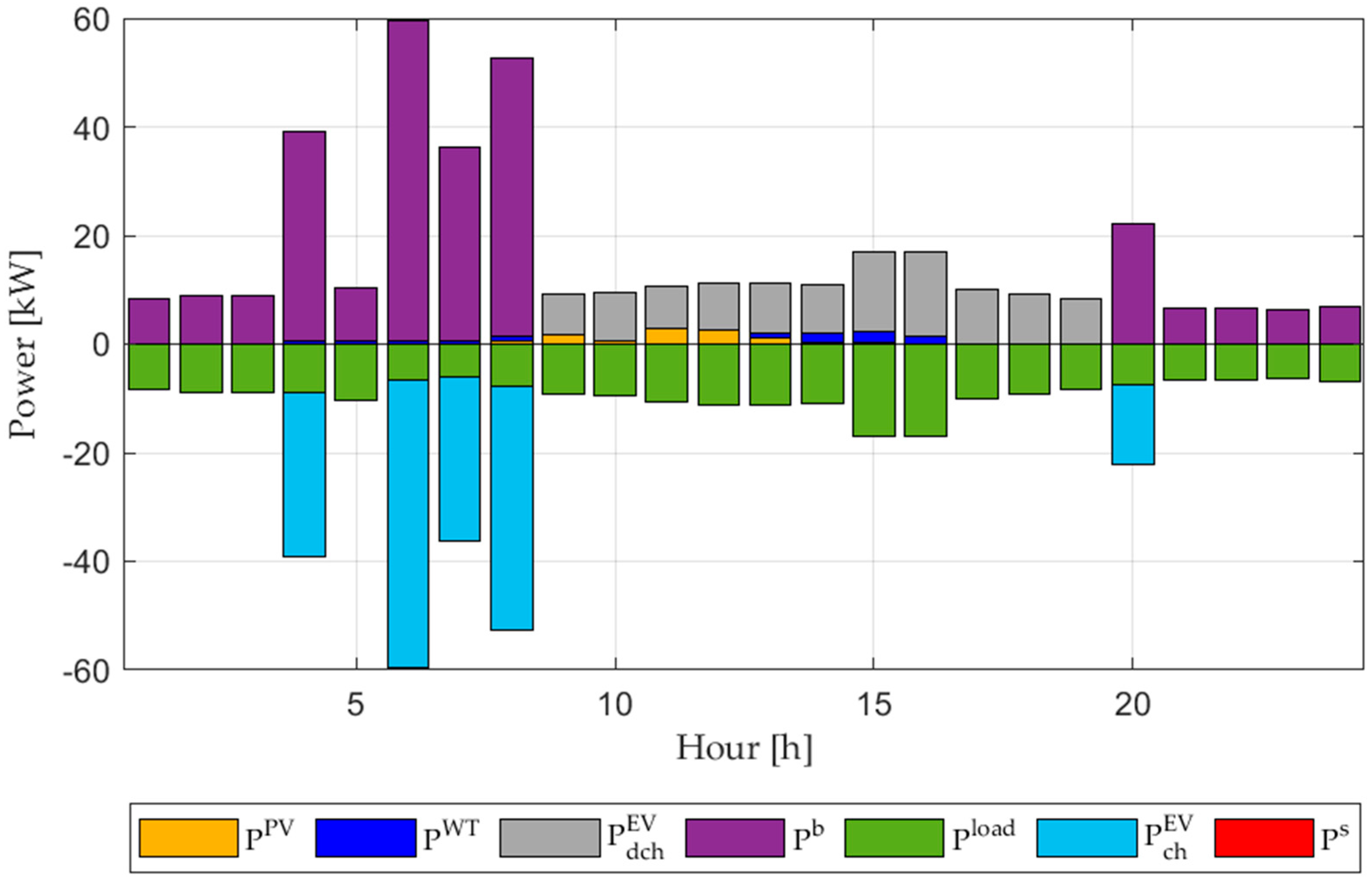
3.2. EMS Results: Sensitivity on the Number of EDVs

This subsection presents the main energy and economic results related to the sensitivity analysis carried out by varying the number of EDVs (N) from 10, passing through to 50 and then up to 100. The annual results are summarized in

Table 4. Annual results.

	[-]	NEDV = 10	NEDV = 50	NEDV = 100
PV active energy generation	[kWh]	39,102
PV curtailed energy	[kWh]	0
PV reactive energy generation	[kVArh]	44,654
WT active energy generation	[kWh]	13,996
WT curtailed energy	[kWh]	0
WT reactive energy generation	[kVArh]	27,503
Bought active energy	[kWh]	34,209	73,585	124,630
Sold active energy	[kWh]	14,604	0	0
Bought reactive energy	[kVArh]	0
Energy charged to EDVs	[kWh]	21,700	62,536	113,581
Energy discharged from EDVs	[kWh]	84,985
NCs	[EUR]	8944	19,868	33,650

.

The capability curves of the inverters connected to the PV and to the WT unit are shown in Figure 3 and Figure 4, where Q^PV and Q^WT, respectively, represent $Q_t^{PV,out}$ and $Q_t^{WT,out}$, while P^PV and P^WT refer to $P_t^{PV,out}$ and $P_t^{WT,out}$. Both the actual curve and the linearized one are depicted in the figures. As previously mentioned, the linearized curve has been modelled in order to be able to use linear programming models. As it is evident from the pictures, for a few hours during the whole year, the inverters are saturated or overloaded. The two figures do not report the second quadrant since no inductive reactive power is absorbed by RES plants in the case study. The provision of reactive power by RES allows zero reactive energy withdrawal from the distribution network in all the examined scenarios. Due to the fact the RES plants almost never produce the maximum active power, it is not necessary to apply curtailment to provide reactive power within the constraints of the linearized capability curve. As far as the injection of active power into the distribution network is concerned, surplus generation from RES only occurs in the scenario with 10 vehicles, whereas in the other two scenarios, this surplus is used to charge the most numerous vehicles.

3.3. Comparison of EMS Results Taking into Account Forecasting Uncertainty

The present subsection presents the main results of the EMS over the whole year when varying the number of EOHs of the two RES power plants in accordance with the correction coefficient introduced in order to take into account the forecasting uncertainty of RES production. The number of EDVs has been considered equal to 50.

The main results are reported in

Table 5. Annual results for different scenarios.

	[-]	Scenario I	Scenario II	Scenario III	Scenario IV
PV active energy generation	[kWh]	41,046	41,046	37,507	37,507
PV curtailed energy	[kWh]	0	0	0	0
PV reactive energy generation	[kVArh]	43,601	42,850	45,753	44,837
WT active energy generation	[kWh]	15,424	12,820	15,424	12,820
WT curtailed energy	[kWh]	0	0	0	0
WT reactive energy generation	[kVArh]	28,556	29,307	26,402	27,321
Bought active energy	[kWh]	70,034	72,737	73,817	76,527
Sold active energy	[kWh]	0	0	0	0
Bought reactive energy	[kVArh]	0	0	0	0
Energy charged to EDVs	[kWh]	61,845	62,228	62,783	63,191
Energy discharged from EDVs	[kWh]	79,872	82,708	86,813	89,828
NCs	[EUR]	18,909	19,639	19,931	20,662

.

According to the previously defined scenarios, the RES production is alternatively increased and reduced when compared to the historical data considered in the base scenario. Scenario I is characterized by increased RES production when compared to the base scenario, leading to a reduced energy exchange between the EDVs and the building; Scenario I is also characterized by the lowest NCs. Scenario IV presents reduced RES production to emulate the possible over-estimation of RES production in the base scenario; in this configuration, the NCs are the highest among all the scenarios, and the exchange of active energy between the EDVs and the building is large because the V2B facility has to compensate for the lack of renewable energy. For the same reason, the amount of energy bought from the network is the highest as well. Scenario II and Scenario III represent intermediate scenarios, with moderate values of NCs, V2B energy exchange and energy purchased from the network. In all scenarios, active energy is never sold to the network due to the large transportation demand of EDVs.

It is important to highlight that the aim of the present study is to simulate the annual operation of the building in order to investigate the benefits deriving from RES generation and V2B techniques: for this reason, the proposed EMS is not designed as a real-time EMS; instead, it is developed in order to be run for the 8760 h of a whole year in order to make global technical and economic considerations. As evident from the results, possible uncertainty in the forecasting of RES generation has a limited impact on the NCs (−4.8% in Scenario I and +4% in Scenario IV). Even variation in the energy exchange between the building and EDVs is limited: in Scenario I, V2B flow is reduced by −6%, and the B2V flow is reduced by −1.1%; in Scenario IV, V2B exchange is increased by +5.4% while the B2V exchange is increased by +1.05%.

3.4. Comparison of EMS Results for Different Typical Days

The present subsection shows the daily results of the EMS for four typical days, defined according to the combination of two criteria: working day/holiday and high RES production/low RES production. For this analysis, the number of EDVs has been considered equal to 50. Regarding EOHs, the base scenario with no uncertainty has been selected.

The days that have been selected according to the aforementioned criteria are summarized in

Table 6. Typical days.

	Working Days	Holidays
Low RES production	Wednesday in December	Sunday in October
	19.56 kWh	45.11 kWh
	Figure 5	Figure 6
High RES production	Friday in June	Sunday in September
	379.73 kWh	366.73 kWh
	Figure 7	Figure 8

, highlighting the energy production of the RES sources.

Figure 5, Figure 6, Figure 7 and Figure 8 show the optimal active power profiles determined using the EMS for the selected days. In these figures, the power associated with EDVs is considered positive when the vehicles are in discharge mode, whilst the charging of the EDVs is considered as a load and, therefore, associated with negative values.

During the working day with low RES penetration (see Figure 5), it is evident that in order to satisfy the transportation demand of the EDVs, power has to be bought from the network. The purchase of electricity from the network is very significant, especially during the night and early in the morning, for two main reasons: one is that the PV unit is not working and the WT is delivering a very low power; the second reason is that EDVs-II (mainly, but also EDVs-I in some hours) are used as “mobile” BESSs: once they have reached the facility after having fulfilled their duty, they are recharged in order to exploit the low off-peak electricity price, and then they are discharged during the day, to avoid buying electricity from the network. When the RES production is very low, a part of the purchased energy is used to charge the EDVs-I so that they are able to satisfy their transportation demand during the day.

During holidays with low RES production (see Figure 6), a large amount of energy must again be purchased from the network, using EDVs as storage systems and exploiting their full availability at the facility throughout the day. Since during holidays, the transportation demand is set to 0, the purchased energy is lower when compared to working days.

During working days with high RES penetration (see Figure 7), it is evident that a much lower power has to be purchased from the network. Thanks to the high RES generation, the EDVs are not discharged during the day, but they are (globally) continuously charged in order to satisfy the transportation demand. The only hours when a more significant amount of power is taken from the network are during the night in order to allow EDVs-II to carry out their service.

Finally, during holidays with high RES penetration (see Figure 8), some energy is bought from the network at the beginning of the day and stored in the EDVs to be used for the services of the following day. During the day, the EDVs are continuously charged in order to avoid the curtailment of RESs, to which a minimal, but still existing, cost is associated.

There is never an excess of electricity sold to the network; this is due to the large number of EDVs that, when exploiting B2V service, charge their batteries in order to use the stored energy to satisfy transportation demands.

V2B services are convenient and have a significant role when RES penetration is low; therefore, they can be used primarily during the winter in order to avoid the purchase of electricity from the network, especially during peak hours, when the cost of energy is higher.

4. Conclusions

The purpose of the present paper was to develop an EMS for the efficient management of a prosumer building connected to the distribution network. The building is owned by the postal service and is equipped with two RESs, namely a PV system and a WT unit, and is equipped with a large fleet of EDVs for postal delivery that can be charged at dedicated charging points installed at the facility. The primary goal of the EMS is to minimize the overall costs associated with the operation of the building, such as those related to the exchange of active and reactive power between the distribution network and the building over the whole year.

Three sensitivity analyses were developed. The first analysis aimed to evaluate the impact of the number of EDVs on the operation of the building while also comparing the annual energy quantities and the NCs. The fleet of EDVs was considered to be composed of either 10, 50 or 100 vehicles. The second analysis was performed in order to evaluate the impact of RES generation forecasting errors on the operation of the building; when considering a number of EDVs equal to 50, the PV and WT generations were alternatively scaled up and down in order to emulate possible underestimations and overestimations in terms of RES forecasting. Then, a third analysis was carried out to analyse the behaviour of the building and the optimal active power profiles with a number of EDVs equal to 50 when considering four different typical days, as identified according to RES generation (high or low) and the considered day (working day or holiday). Moreover, the impact of errors in forecasting renewable energy production on the EMS results was also investigated.

This paper showed how increasing the dimension of the EDV fleet affected energy and cost, highlighting the fact that V2B applications are necessary in order to fully exploit the consumption of RES-derived energy.

Future developments could involve the modification of the load profile of the building and the behaviour of the EDVs in terms of availability and transportation demand in order to investigate different scenarios and different types of users. In addition, to expand the proposed EMS, other technical implementations could also be included, such as the possibility for EVs to exchange reactive power with the building and the implementation of a model of the building’s electric network in order to take power losses into account.

References

1. IEA. Buildings; IEA: Paris, France, 2022. [Google Scholar]
2. Renovation Wave: Creating Green Buildings for the Future. Available online: https://europa.eu/!bG4m7p (accessed on 16 June 2023).
3. Fit for 55: Why the EU Is Toughening CO2 Emission Standards for Cars and Vans. Available online: https://europa.eu/!w39R7x (accessed on 16 June 2023).
4. Fiaschi, D.; Bandinelli, R.; Conti, S. A case study for energy issues of public buildings and utilities in a small municipality: Investigation of possible improvements and integration with renewables. Appl. Energy 2012, 97, 101–114. [Google Scholar] [CrossRef]
5. Alshahrani, A.; Omer, S.; Su, Y.; Mohamed, E.; Alotaibi, S. The technical challenges facing the integration of small-scale and large-scale PV systems into the grid: A critical review. Electronics 2019, 8, 1443. [Google Scholar] [CrossRef]
6. Walker, S.L. Building mounted wind turbines and their suitability for the urban scale—A review of methods of estimating urban wind resource. Energy Build. 2011, 43, 1852–1862. [Google Scholar] [CrossRef]
7. Gautier, A.; Jacqmin, J.; Poudou, J.-C. The prosumers and the grid. J. Regul. Econ. 2018, 53, 100–126. [Google Scholar] [CrossRef]
8. Lopez, A.; Ogayar, B.; Hernández, J.; Sutil, F. Survey and assessment of technical and economic features for the provision of frequency control services by household-prosumers. Energy Policy 2020, 146, 111739. [Google Scholar] [CrossRef]
9. Parag, Y.; Sovacool, B.K. Electricity market design for the prosumer era. Nat. Energy 2016, 1, 16032. [Google Scholar] [CrossRef]
10. Lavi, Y.; Apt, J. Using PV inverters for voltage support at night can lower grid costs. Energy Rep. 2022, 8, 6347–6354. [Google Scholar] [CrossRef]
11. Talkington, S.; Grijalva, S.; Reno, M.J.; Azzolini, J.A. Solar PV inverter reactive power disaggregation and control setting estimation. IEEE Trans. Power Syst. 2022, 37, 4773–4784. [Google Scholar] [CrossRef]
12. Piazza, G.; Bracco, S.; Delfino, F.; Siri, S. Optimal design of electric mobility services for a Local Energy Community. Sustain. Energy Grids Netw. 2021, 26, 100440. [Google Scholar] [CrossRef]
13. Ioakimidis, C.; Thomas, D.; Rycerski, P.; Genikomsakis, K. Peak shaving and valley filling of power consumption profile in non-residential buildings using an electric vehicle parking lot. Energy 2018, 148, 148–158. [Google Scholar] [CrossRef]
14. Barone, G.; Buonomano, A.; Forzano, C.; Giuzio, G.F.; Palombo, A. Increasing self-consumption of renewable energy through the Building to Vehicle to Building approach applied to multiple users connected in a virtual micro-grid. Renew. Energy 2020, 159, 1165–1176. [Google Scholar] [CrossRef]
15. Arias, N.B.; Hashemi, S.; Andersen, P.B.; Træholt, C.; Romero, R. Distribution system services provided by electric vehicles: Recent status, challenges, and future prospects. IEEE Trans. Intell. Transp. Syst. 2019, 20, 4277–4296. [Google Scholar] [CrossRef]
16. Borge-Diez, D.; Icaza, D.; Açıkkalp, E.; Amaris, H. Combined vehicle to building (V2B) and vehicle to home (V2H) strategy to increase electric vehicle market share. Energy 2021, 237, 121608. [Google Scholar] [CrossRef]
17. Martinenas, S.; Marinelli, M.; Andersen, P.B.; Træholt, C. Implementation and demonstration of grid frequency support by V2G enabled electric vehicle. In Proceedings of the 2014 49th International Universities Power Engineering Conference (UPEC), Cluj-Napoca, Romania, 2–5 September 2014; pp. 1–6. [Google Scholar]
18. Meng, J.; Mu, Y.; Jia, H.; Wu, J.; Yu, X.; Qu, B. Dynamic frequency response from electric vehicles considering travelling behavior in the Great Britain power system. Appl. Energy 2016, 162, 966–979. [Google Scholar] [CrossRef]
19. Aziz, M.; Oda, T.; Kashiwagi, T. Extended utilization of electric vehicles and their re-used batteries to support the building energy management system. Energy Procedia 2015, 75, 1938–1943. [Google Scholar] [CrossRef]
20. Zhou, Y.; Cao, S.; Hensen, J.L.; Lund, P.D. Energy integration and interaction between buildings and vehicles: A state-of-the-art review. Renew. Sustain. Energy Rev. 2019, 114, 109337. [Google Scholar] [CrossRef]
21. Zheng, S.; Huang, G.; Lai, A.C. Coordinated energy management for commercial prosumers integrated with distributed stationary storages and EV fleets. Energy Build. 2023, 282, 112773. [Google Scholar] [CrossRef]
22. He, Z.; Khazaei, J.; Freihaut, J.D. Optimal integration of Vehicle to Building (V2B) and Building to Vehicle (B2V) technologies for commercial buildings. Sustain. Energy Grids Netw. 2022, 32, 100921. [Google Scholar] [CrossRef]
23. Kelm, P.; Mieński, R.; Wasiak, I. Energy management in a prosumer installation using hybrid systems combining EV and stationary storages and renewable power sources. Appl. Sci. 2021, 11, 5003. [Google Scholar] [CrossRef]
24. Rücker, F.; Schoeneberger, I.; Wilmschen, T.; Sperling, D.; Haberschusz, D.; Figgener, J.; Sauer, D.U. Self-sufficiency and charger constraints of prosumer households with vehicle-to-home strategies. Appl. Energy 2022, 317, 119060. [Google Scholar] [CrossRef]
25. Thomas, D.; Deblecker, O.; Ioakimidis, C. Optimal operation of an energy management system for a grid-connected smart building considering photovoltaics’ uncertainty and stochastic electric vehicles’ driving schedule. Appl. Energy 2018, 210, 1188–1206. [Google Scholar] [CrossRef]
26. Farinis, G.Κ.; Kanellos, F.D. Integrated energy management system for Microgrids of building prosumers. Electr. Power Syst. Res. 2021, 198, 107357. [Google Scholar] [CrossRef]
27. Bracco, S.; Fresia, M. Energy Management System for the Optimal Operation of a Grid-Connected Building with Renewables and an Electric Delivery Vehicle. In Proceedings of the IEEE EUROCON 2023—20th International Conference on Smart Technologies, Torino, Italy, 6–8 July 2023; pp. 472–477. [Google Scholar]
28. Lofberg, J. YALMIP: A toolbox for modeling and optimization in MATLAB. In Proceedings of the 2004 IEEE International Conference on Robotics and Automation (IEEE Cat. No. 04CH37508), Taipei, Taiwan, 2–4 September 2004; pp. 284–289. [Google Scholar]
29. Šúri, M.; Huld, T.; Cebecauer, T.; Dunlop, E.D. Geographic aspects of photovoltaics in Europe: Contribution of the PVGIS web site. IEEE J. Sel. Top. Appl. Earth Obs. Remote Sens. 2008, 1, 34–41. [Google Scholar] [CrossRef]
30. de Simón-Martín, M.; Bracco, S.; Piazza, G.; Pagnini, L.C.; González-Martínez, A.; Delfino, F. Application to Real Case Studies. In Levelized Cost of Energy in Sustainable Energy Communities: A Systematic Approach for Multi-Vector Energy Systems; Springer International Publishing: Cham, Switzerland, 2022; pp. 77–120. [Google Scholar] [CrossRef]
Figure 1. Electric system scheme.
Energies 16 07213 g001
Figure 2. Capability curve linearization for RES plants (a) and distribution network coupling (b).
Energies 16 07213 g002
Figure 3. PV inverter capability curve. Blue circles represent the hourly operating points of the inverter. The red circular line represents the non-linearized capability curve of the inverter. The yellow line represents the sloped portion of the linearized capability curve of the inverter.
Energies 16 07213 g003
Figure 4. WT inverter capability curve. Blue circles represent the hourly operating points of the inverter. The red circular line represents the non-linearized capability curve of the inverter. The yellow line represents the sloped portion of the linearized capability curve of the inverter.
Energies 16 07213 g004
Figure 5. Active power profiles of the 4 December.
Energies 16 07213 g005
Figure 6. Active power profiles of the 6 October.
Energies 16 07213 g006
Figure 7. Active power profiles of the 7 June.
Energies 16 07213 g007
Figure 8. Active power profiles of the 29 September.
Energies 16 07213 g008