Abstract
As a result of ever-growing energy demands, motor vehicles are among the largest contributors to overall energy consumption. This has led researchers to focus on fuel consumption, which has important implications for the environment, the economy, and geopolitical stability. This article presents a comprehensive analysis of various fuel consumption modeling methods, with the aim of identifying parameters that significantly influence fuel consumption. The scientific novelty of this article lies in its use of low-cost technology, i.e., an OBD-II interface paired with a mobile phone, combined with modern mathematical modeling methods to create an accurate model of the fuel consumption of a vehicle. A vehicle test drive was performed, during which variations in selected parameters were recorded. Based on the obtained data, a model of the vehicle’s fuel consumption was built using three forecasting methods: a multivariate regression model, decision trees, and neural networks. The results show that the multivariate regression model obtained the lowest MSE, MAR, and MRSE coefficients, indicating that this was the best forecasting method among those tested. Sufficient forecast error results were obtained using neural networks, with increases of approximately 73%, 10%, and 131% in MSE, MAE, and MRAE, respectively, compared to regression results. The worst results were obtained with the decision tree model, with increases of approximately 163%, 21%, and 92% in MSE, MAE, and MRAE compared to the regression results.
Keywords:
fuel consumption; OBD-II; mobile phone; GPS; signal processing; regression; decision trees; neural networks 1. Introduction
Transportation plays an important role in the global economy by facilitating the movement of people and goods over distances. As a result, the transport industry continues to experience increasing energy demands. Among the largest contributors to overall energy consumption is motor vehicles. Increased energy consumption is stimulating interest in the field of fuel consumption due to the huge impact of this factor on the economy, environment, geopolitical stability, and national security of individual countries [1].
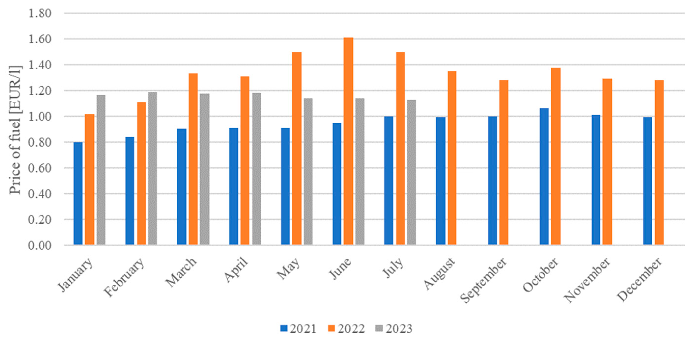
The financial stability of households and enterprises is an important factor in ensuring national security [2]. It enables the collection of funds and resources that are necessary for the state to guarantee its ability to effectively counteract threats to the internal environment and the external socioeconomic system [3]. A major threat to financial security is inflation, which increases prices and thus reduces the purchasing power of consumers. Currently, many factors have a significant impact on increasing inflation. The main ones include supply disruptions related to the COVID-19 pandemic and the resulting disruption of global supply chains, as well as sharp increases in energy, fuel, and food prices resulting from the war in Eastern Europe [4]. On average, European Union (EU) countries recorded an increase in inflation from 0.5% in 2020 to 8.8% in 2022. The largest increases were recorded in the Baltic states, Lithuania, Latvia, and Estonia (up to approximately 18%), while the lowest was in France (about 5.2%) [5]. The increased inflation and the accompanying economic slowdown (associated with the risk of undermining financial security) were mainly caused by increased fuel prices in global markets. The main reasons for this phenomenon are the reduced processing capacity of refineries located in Europe (in connection with the plan to switch to green transport), reduced fuel exports by China in 2022, reduced production by the Organization of the Petroleum Exporting Countries (OPEC), and the economic sanctions imposed on Russia by the EU. Fluctuations in fuel prices in Poland are shown in Figure 1. Fuel prices per liter in the EU ranged from an average of EUR 12 in 2021 to a peak of EUR 1.88 in 2022, with a current average of EUR 1.61 [6]. An analysis of the chart below indicates a significant increase in fuel prices at the beginning of 2022. Currently, a downward trend in fuel prices can be observed, but they are still at a higher level than before the start of the war in Eastern Europe.

Figure 1.
Fuel prices in Poland in 2021–2023 [6].
It is important to analyze fuel prices because, in Europe, a significant percentage of cars are dependent on fossil fuels, such as petrol and diesel; 36.4% of all newly registered cars in the EU run on petrol, while diesel accounts for 16.4% of registrations. Additionally, 21.6% of new passenger cars in the EU are electric vehicles, while hybrids account for 22.6% of total car sales [7].
Fuel consumption has a very significant impact on the costs incurred by households and enterprises, as well as on the emission of harmful pollutants into the environment, exacerbating the greenhouse effect. For example, in the US, nearly one-fifth of all CO2 emissions is generated by cars and trucks, and the entire transportation sector is responsible for nearly 30% of all US global warming gas emissions [8]. Fuel consumption has several adverse effects on the environment, including air and water pollution, the greenhouse effect, and landscape degradation, with the loss of natural habitats. In addition to these environmental effects, dependence on fossil fuels can have significant economic and political implications, because many countries depend on such fuels for their economy (potentially leading to international conflicts and tensions). Volatility in oil and other prices can have a negative impact on the global economy. Rising fuel prices caused by, among other things, unstable geopolitical situations and declarations regarding sustainable development, make it important to take actions that will lead to the identification of factors influencing fuel consumption by vehicles and its consequent minimization. Another reason why it is important to assess fuel consumption is that there is a limited amount of crude oil available in the world and the volume of production of vehicles that use alternative energy sources is currently insufficient [9].
Taking into account the above factors, it is important to take measures to reduce fuel consumption during vehicle operation. This is possible by determining factors and parameters that affect increased fuel consumption and by implementing appropriate management strategies to optimize the costs incurred. That became both the scientific and practical goal of this study.
Fuel consumption in motor vehicles is influenced by vehicle design and technology, including the following factors: vehicle materials (aluminum coating on a car body can reduce fuel consumption by up to 13% on hot days by limiting the use of air-conditioning) and vehicle weight (increased weight leads to increased fuel consumption); aerodynamics (lower drag coefficients reduce fuel consumption); engine design, type, and technology (diesel vehicles consume about 12% less fuel than gasoline-fueled vehicles); and the transmission system (more advanced transmission systems, e.g., CVTs and DCTs, have improved fuel consumption compared to traditional systems). However, technical improvements leading to more fuel-efficient cars will not always result in overall reduced fuel consumption. This is because many car buyers prioritize size and power over fuel economy. Fuel economy is more important to used car buyers [10,11], while for new car buyers, this factor is not the most important [12,13].
Several external factors can impact fuel consumption in motor vehicles, including weather conditions (ambient temperature, both high and low, affects fuel consumption), road type and surface conditions (uneven terrain and the presence of hills lead to increased engine load and rolling resistance, which directly increases fuel consumption), altitude (air density is reduced in higher altitudes air density, which can decrease fuel consumption), and traffic congestion (repeated acceleration and deceleration will increase fuel consumption) [10]. Unfortunately, a driver moving along a predetermined and planned route has no influence on any of these factors [10,13].
On the other hand, the following driver behaviors can significantly lower fuel consumption: using smooth acceleration and gentle braking, as opposed to rapid acceleration and hard braking; using cruise control, which can help to maintain a constant speed (thus maintaining a constant engine load and preventing fluctuations) and optimize fuel consumption; engine braking, or using the vehicle’s momentum to maintain speed; avoiding aggressive driving such as rapid lane changes and tailgating; and using efficient gear shifting by timely upshifting and downshifting, which maintains optimal engine RPMs in manual transmission vehicles [14].
Proper vehicle maintenance is essential in order to achieve optimal fuel consumption and overall vehicle performance. It includes, among other things, regular oil changes (which reduces engine friction), proper tire inflation and alignment (which reduces rolling resistance), air filter replacement (which maintains engine performance), and the use of diagnostic tools, such as OBD-II scanners (which monitor various vehicle parameters in real-time).
Many drivers develop their driving habits after taking a driving course; often, these habits initially have a negative impact on the vehicle, and also result in increased fuel consumption (e.g., exceeding the speed limit, accelerating or braking suddenly, etc.). Over time, drivers gain experience and their driving style becomes more balanced. However, this process can be significantly accelerated with the use of currently available technology, such as mobile phones and OBD-II scanners. These devices enable selected parameters of the vehicle to be displayed and read in real-time. Analyzing these data allows the construction of fuel consumption models for specific vehicles, and understanding them can support drivers in practicing economical driving.
Literature Review on Fuel Consumption Modeling
The literature analysis showed that fuel consumption modeling is a problem often addressed in scientific publications. Fuel consumption is typically expressed in liters per hundred kilometers (L/100 km) or miles per gallon (mpg). Various models exist to predict fuel consumption based on different factors, and they can be divided into the following categories: engine map-based models, which are accurate but require extensive data for every car; regression-based models, which are developed based on regression results from experiments but have limited physical interpretation; load-based models, which are based on physical equations for describing phenomena that affect fuel consumption but are computationally intensive; and hybrid models, the most frequently used models, which combine features of the above-mentioned models to optimize computation time and accuracy [10].
A problem often described in the literature is how driving style can influence fuel consumption [15]. These studies often used the OBD-II interface to obtain the data necessary for analysis [16,17,18]. Alessandrini et al. indicated that it is possible to develop a modern method that identifies the relationship between fuel consumption and the type of road network covered or even specific vehicle users [19]. Ericsson, on the other hand, pointed out that increased fuel consumption is significantly affected by sudden changes in vehicle acceleration and high speed, especially exceeding 100 km/h. The significant impact of the vehicle’s technical conditions was also discussed [20]. Meseguer et al. noted that reducing fuel consumption is influenced by minimizing the duration of driving in low gears and using the higher gears as soon as possible while limiting continuously changing gears [21].
The regression-based studies available in the literature can be divided according to the type of method used to estimate fuel consumption. Machine learning models based on support vector machines [9,22], neural networks [23], or decision trees [24] are widely used. Some studies also use fuzzy logic algorithms [25] or classical regression for modeling [26].
Fuel consumption can be modeled with the use of analytical, statistical, or experimental techniques. Hien et al. [27] conducted a predictive study of fuel consumption and carbon dioxide emissions by constructing a model to predict changes in the near future. With the use of descriptive and inferential statistics, a comprehensive outlook of fuel consumption variation based on dimensional and technical factors was given. Machine learning and deep learning techniques also enabled the determination of a correlation between vehicle specifications and total fuel consumption as a single input–single output or multiple input–single output relation.
Bifulco et al. [28] developed a model for computing instantaneous fuel consumption based on data from the vehicle’s OBD-II port. The analysis was aimed at validating the model performance taking into account different factors and determining the percentage deviation between predicted values given by the model and observed values. The authors showed that instantaneous fuel consumption could be predicted with the use of various models based on a few input variables, and better estimations could be obtained when values were aggregated into fairly long time windows.
Zhao et al. [29] conducted a study of methods to predict vehicle fuel consumption by means of algorithms and statistical models, including neural networks and traditional machine learning. According to the authors, the estimation model for fuel consumption based on neural networks had high accuracy only if the input data were sufficient. Also, the use of hybrid fuel consumption models, consisting of multiple machine learning methods, was found to lead to more reliable results.
According to the analysis Abediasl et al. [30] performed with the use of on-board diagnostics (OBD-II) data, machine learning algorithms using the random forest (RF) technique produced more accurate predictions compared to other tested techniques, including gradient boosting and neural networks.
In conclusion, several modern, complex tools are used to model the discussed problem, including machine learning, or deep learning, but there is a noticeable lack of studies using simple mathematical models, such as regression models, and comparing the effectiveness of their predictions with more advanced models. In addition, simple regression models enable a thorough analysis of the degree of influence of individual explanatory variables on fuel consumption, which is not possible with the use of machine learning models or neural networks. Therefore, the aim of this study was to model vehicle fuel consumption using three methods—regression, decision trees, and neural networks—based on the data provided by a low-cost OBD-II interface.
2. Materials and Methods
On-Board Diagnostic II (OBD-II) is a diagnostic system used in cars that enables access to a variety of real-time data related to vehicle performance and emissions. The OBD standard (OBD-I) was introduced in the mid-1990s, and all gasoline cars sold in the EU since 2001 (all diesel cars since 2004) have been required to have an OBD-II system. This system can read information about the vehicle sensor’s status from the engine control unit (ECU) through the use of an OBD-II adapter, which is connected directly to the vehicle [31,32].
2.1. Research Methodology
The OBD-II adapter typically uses various communication standards that allow data exchange. The most common are wireless communication methods (Bluetooth or Wi-Fi), which allow mobile phones to be used to read selected technical parameters of the car. There are also several OBD-II applications available for mobile phone devices, such as Torque Pro (Android; ver. 1.12.101; Ian Hawkins, Newport Pagnell, Buckinghamshire, UK), DashCommand (iOS and Android; ver. 4.8.15; Palmer Performance Engineering, Orem, UT, USA), and EngineLink (iOS; ver. 8.0; K Solution LLC, Phoenix, AZ, USA) [33,34]. Most of OBD-II applications allow monitoring of selected car parameters, and some, including Torque Pro, also allow logging of all available parameters from the ECU, including those of the phone’s built-in sensors [35]. Parameters that can be read from the OBD-II include engine speed, vehicle speed, engine load, engine coolant temperature, fuel pressure, and mass air flow rate. The system enables self-diagnostics, reporting, and real-time vehicle data monitoring. Using the data, OBD-II can provide real-time feedback to drivers, allowing them to make corrections to their driving behavior to optimize fuel consumption.
Although the OBD-II standard is universal for cars currently being manufactured and sold in the European Union, the same technical parameters cannot be read from every car. In this case, a great deal depends on the technical parameters of the car. In addition to reading the technical parameters from the ECU, applications such as Torque Pro enable the recording of data from the integrated GPS module in the mobile phone. This makes it possible to record the vehicle’s path during the trip. Since GNSS (a functional extension of GPS) is a commonly used system for locating and analyzing the movement of vehicles, it is extremely important to determine its accuracy [36,37].
Because they are readily available to the ordinary user and due to the increasing possible uses of electronic devices such as mobile phones, OBD-II interfaces, and mobile applications, the selected technical parameters were acquired in order to build a model of their impact on fuel consumption.
To obtain these data, a test car was selected and was along a route with a total length of approximately 320 km (Warsaw-Rzeszów, Poland) under real traffic conditions. The vehicle used for the road test was a Mazda 3 (Mazda Motor Corporation, Fuchu, Japan) it is shown in Figure 2 and its technical specifications are given in Table 1. The vehicle was driven by one driver. The route was chosen due to the variety of terrain elevation and the presence of urban sections and expressways (different speed limits).

Figure 2.
Mazda 3 sedan with SkyActiv-G 2.0.

Table 1.
Technical specifications of the selected vehicle.
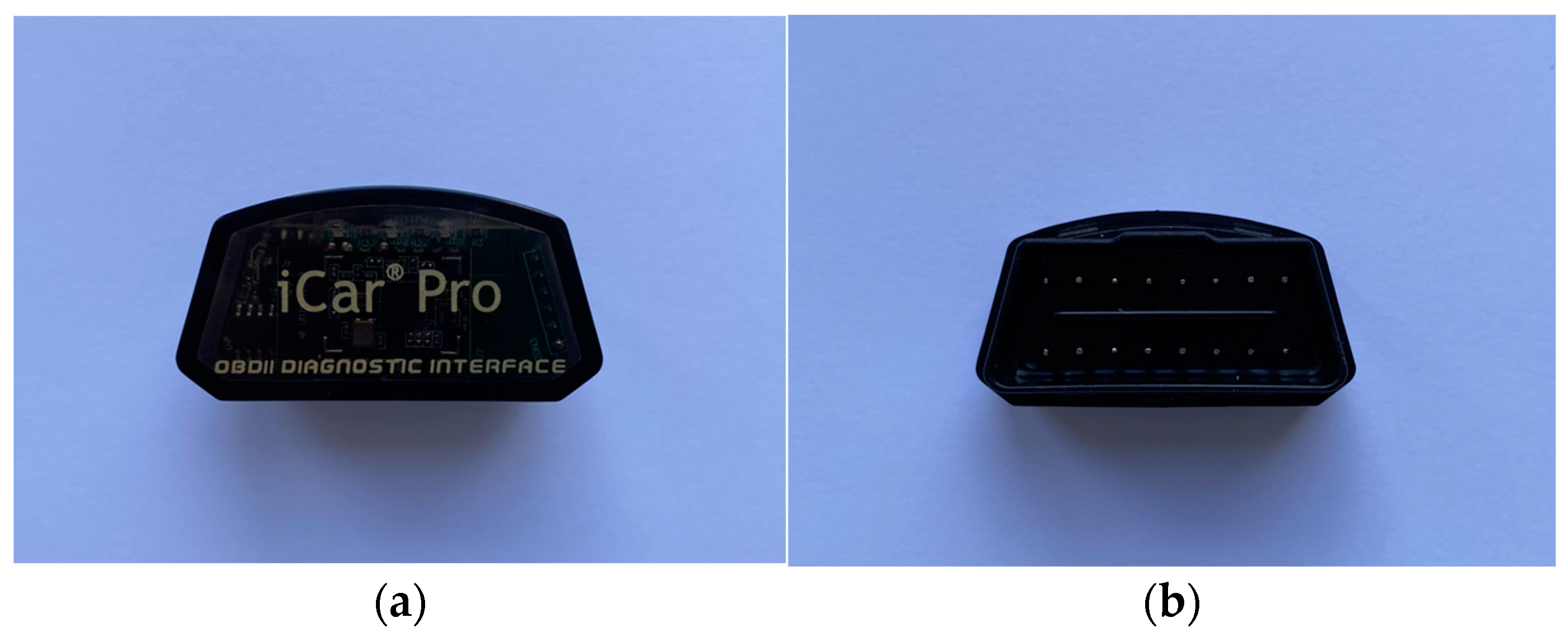
A low-cost (approximately EUR 28) Vgate iCar Pro Wi-Fi OBD-II adapter (Vgate, Shenzhen, China) [37] with the Torque Pro application was used to record the data from the car (Figure 3). A low-cost LG G6 mobile phone (Android OS, release date 2017; LG Electronics, Seoul, Republic of Korea) was used for data logging via Wi-Fi. The sampling frequency of the gathered data was set to 1 Hz (built-in smartphone GPS module limitation).
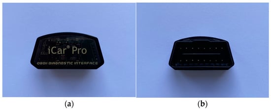
Figure 3.
OBD-II adapter: (a) front view, (b) rear view.
Prior to selecting the parameters for creating the model, an analysis was performed, which indicated many parameters affecting the fuel consumption of a car. Next, the parameters on which the driver has no direct influence were rejected: intake air temperature, engine coolant temperature, etc. However, the final choice of parameters was based on the criterion of readout availability (from the OBD-II or mobile phone) or the possibility of calculating the parameter (indirectly from other variables), because not all relevant parameters (including current gear) are directly available to read from the low-cost OBD-II interface. Finally, the following parameters were selected to build the model: current gear, engine speed, vehicle speed, vehicle acceleration, engine load, and road slope. These variables are presented, categorized by type and the method of obtaining them, in Table 2.
Table 2.
Acquired data specifications.
Basic descriptive statistics of the variables were calculated and the significance of their impact on the modeled dependent variable was assessed (Table 3 and Table 4).
Table 3.
Descriptive statistics of analyzed variables based on OBD data.
Table 4.
Correlation between dependent variable and independent quantitative variables.
Both engine speed (Figure 4) and engine load (Figure 5) were read directly through the OBD-II interface. Engine speed is a significant factor because it is directly related to the operation of the engine: continuous too-high or too-low RPM can cause increased wear and significantly increased fuel consumption.
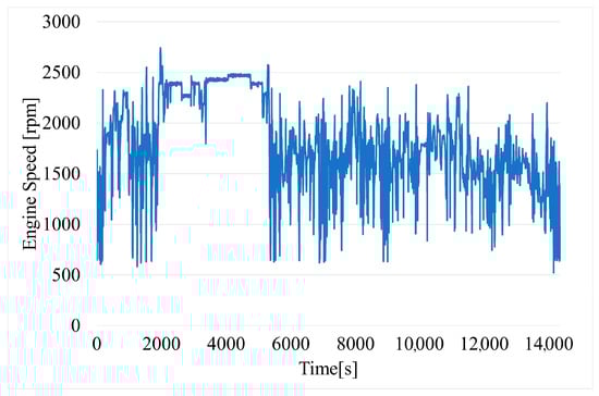
Figure 4.
Time variation of engine speed.
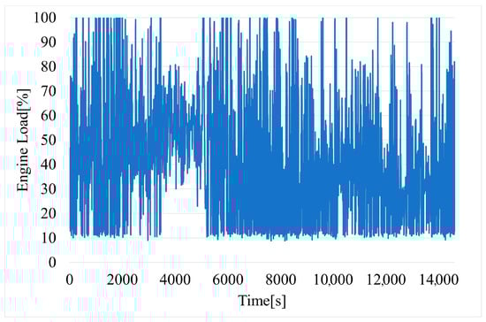
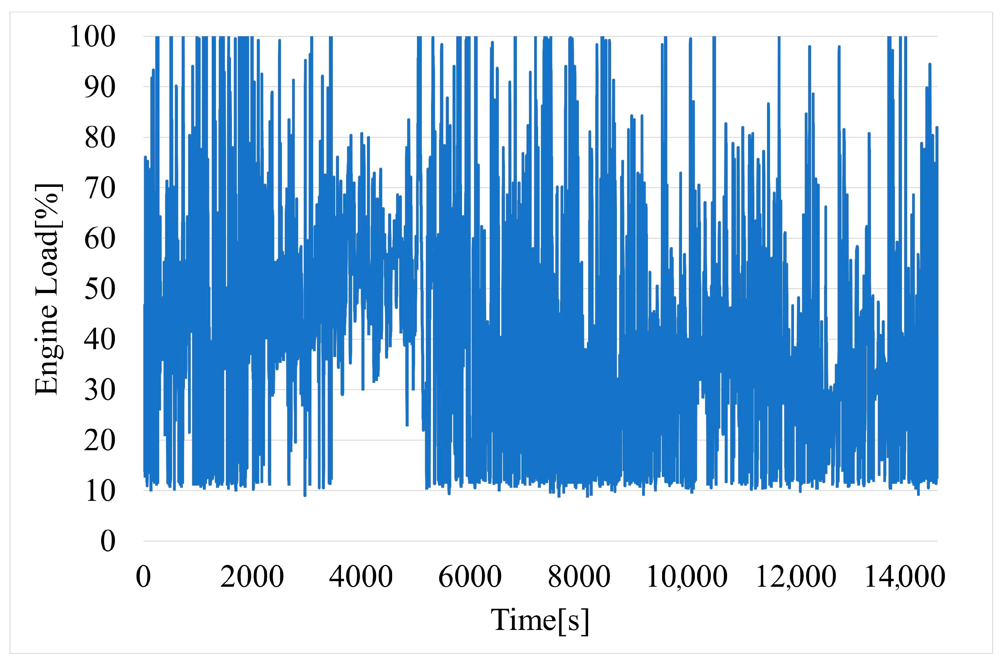
Figure 5.
Time variation of engine load.
Engine load (Figure 5) is commonly expressed as a percentage of the maximum available power. This parameter is computed using mass air flow (MAF), throttle position sensor (TPS), manifold absolute pressure (MAP), engine speed (RPM), and other data. The exact formula can vary based on the vehicle’s ECU, and some of the sensors may not be used for calculation. A high engine load percentage may indicate aggressive driving or driving up inclines, while a low engine load percentage may indicate assertive driving or cruising at a steady speed on a flat surface.
Vehicle speed (Figure 6) is read directly from the phone’s GPS module. This parameter is also available from the OBD-II, but data from GPS are more accurate in this case.
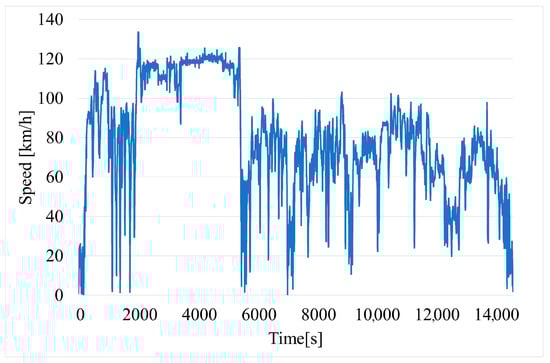
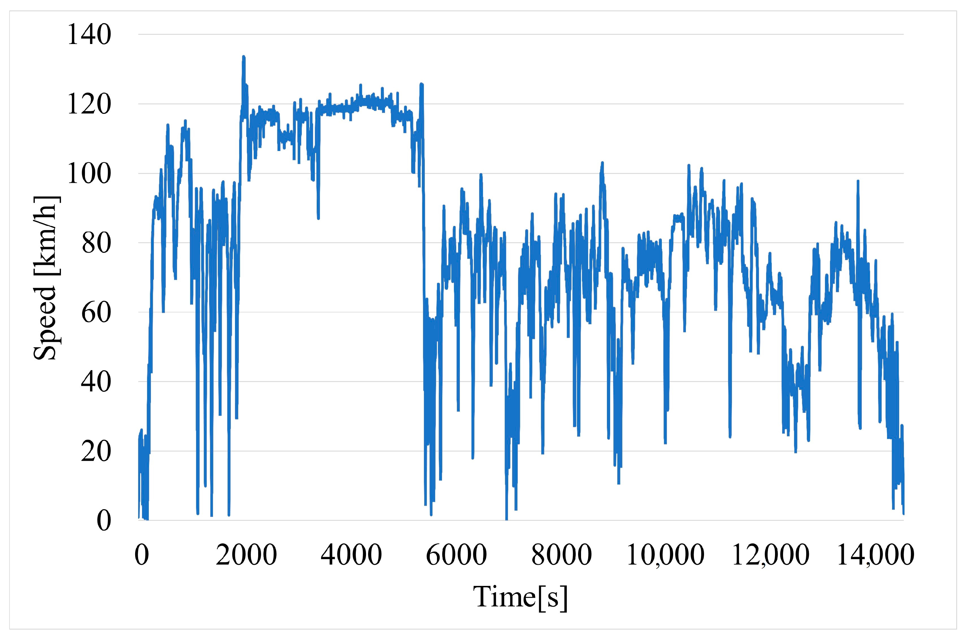
Figure 6.
Time variation of vehicle speed.
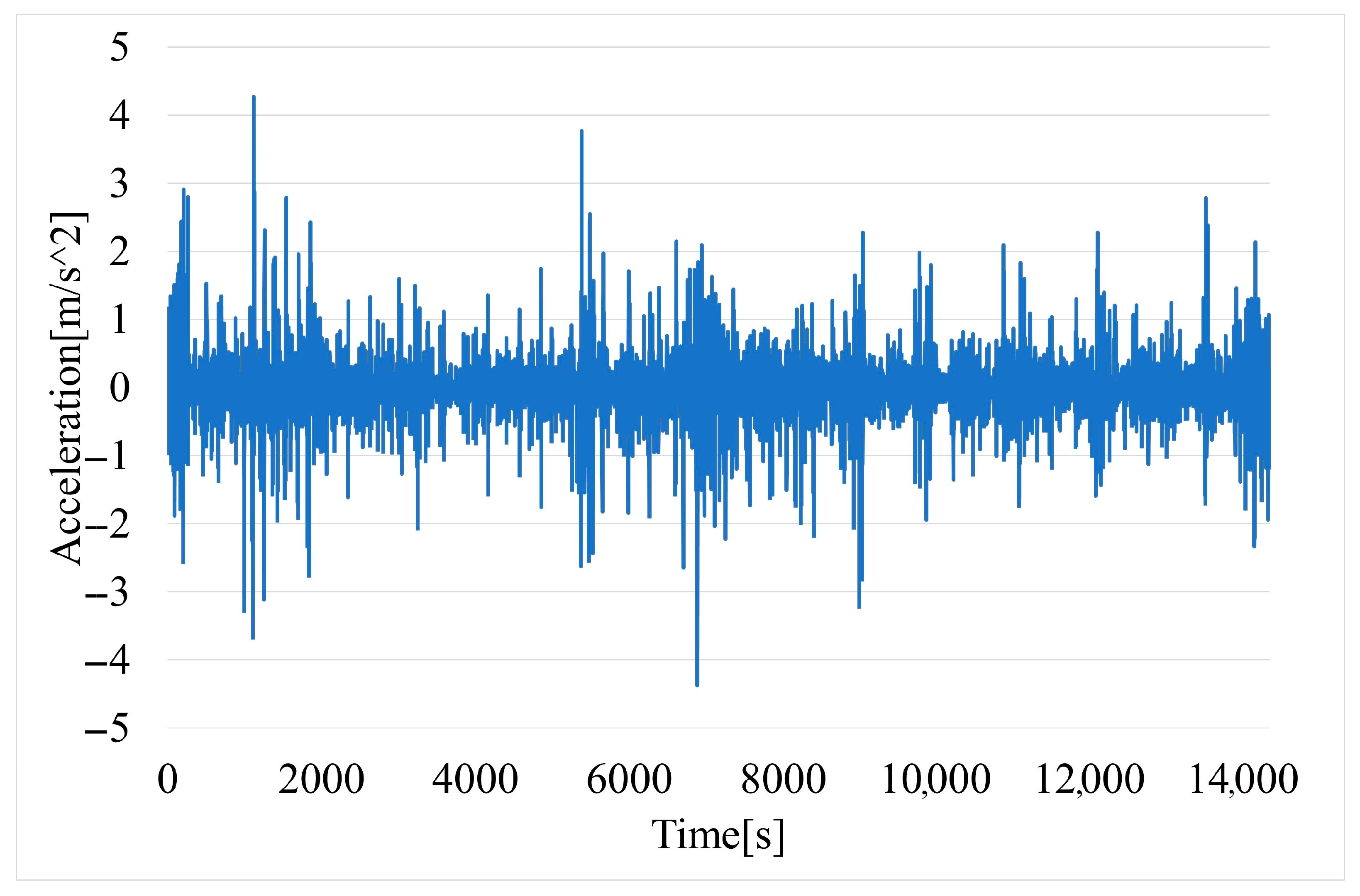
Vehicle acceleration (Figure 7) is determined by differentiating the described vehicle speed readings with respect to time.

Figure 7.
Time variation of vehicle acceleration.
The slope of the road (Figure 8) was determined based on the transformation of the GPS coordinates latitude, longitude, and altitude to north, east, down (NED), which is a geographical coordinate system often used in navigation due to local tangent plane (Earth’s curvature can be ignored for small areas such as roads), its alignment with gravity (the down axis is aligned with gravity), compatibility with GPS (simple conversion form GPS output), etc.
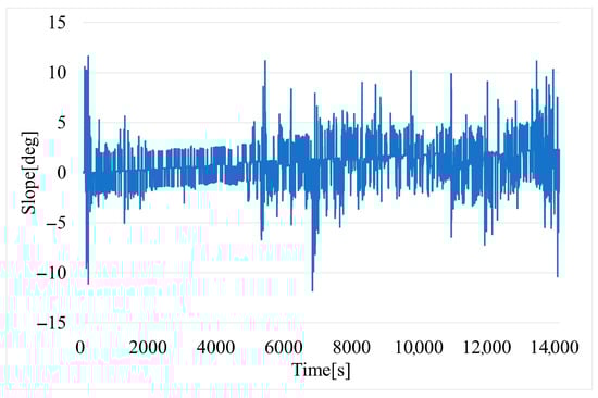
Figure 8.
Time variation of road slope.
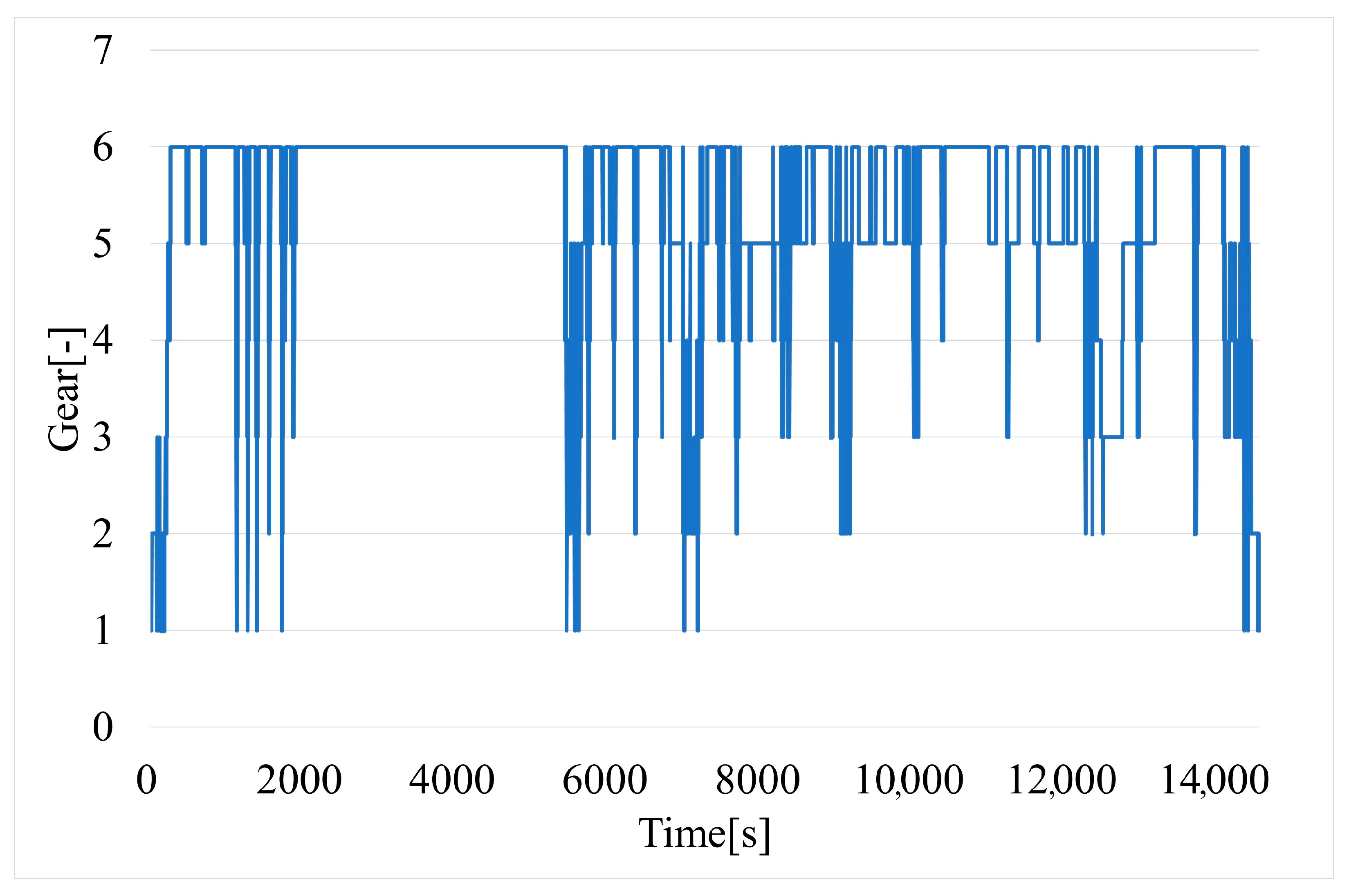
Unfortunately, the current gear is not available from the OBD-II interface (often only for an automatic gearbox). It is possible to determine the current gear (Figure 9) by using linear regression of the obtained dependencies between vehicle speed and engine speed (Figure 10).

Figure 9.
Time variation of current gear of vehicle.
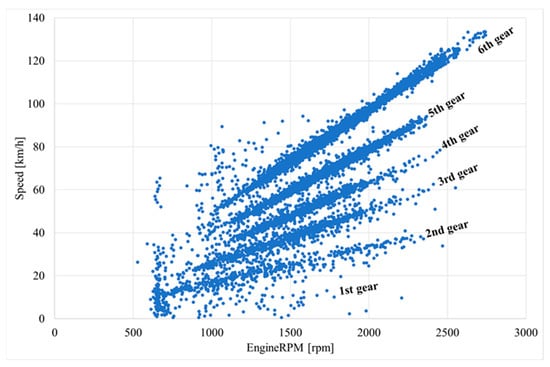
Figure 10.
Vehicle speed variation depending on engine speed, with graphical indication of gears.
The fuel consumption of the vehicle (Figure 11) is calculated based on reading the fuel used (liters) from the OBD-II and the traveled length of road in a given period of time calculated from GPS time stamps.
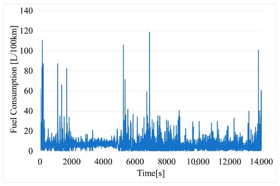
Figure 11.
Time variation of fuel consumption of vehicle.
The results represent raw data that have not been filtered, except for slope (moving average from three measurement points). It was decided to omit the filtering process to assess the quality of the obtained raw data and whether they could be subsequently used in practical solutions operating in real-time.
Since it is not possible to determine fuel consumption in L/100 km when the vehicle is idling (no displacement), the following rule for data selection was adopted: speed > 0 and gear > 0.
2.2. Modeling Methods
Out of all the methods mentioned in the reviewed literature used to determine vehicle fuel consumption, three methods were selected: multiple regression model (Section 2.2.1), decision trees (Section 2.2.2), and neural networks (Section 2.2.3). All three methods require data preprocessing to remove missing values and outliers. Multiple regression assumes linearity, while decision trees and neural networks can model nonlinear relationships. Neural networks require more computational resources and a more complex configuration, including defining the architecture and learning method. Each model was based on the same set of data.
2.2.1. Multiple Regression Model
Multiple regression quantifies the relationship between multiple independent variables and a dependent variable. Including many independent variables in the regression model allows for more accurate and reliable forecasting. It is assumed that the model should contain variables strongly correlated with the dependent variable but at the same time be weakly interdependent. Multiple regression analysis is considered to be an extension of rectilinear regression analysis, with one explanatory variable including a larger number of them [38]. The linear model of multivariate regression is given as Equation (1):
where Y is the expected value of the variable Y, provided that the variable Xi takes the value xi; βj represents the model parameters (regression coefficients); and εi represents internal disturbances.
Model parameters βj are estimated using the least squares method (LSM), based on the assumption that when making the estimation, one should try to minimize the error consisting of differences between observed values yi and model predicted values . The estimated parameters, in accordance with this method, should take values such that the condition for the sample data is met (2):
where yi is the empirical value of variable Y and is the theoretical value determined by the model.
The estimated regression function takes the following form (3):
where i = 1, 2, …, n indicates the observation items numbered consecutively, bj is a regression coefficient, and ei is a residual, defined as the difference between empirical and theoretical values.
Model diagnostics can be performed by residual analysis or collinearity analysis of explanatory variables. Quantitative residual analysis includes testing the normality of the random component distribution (e.g., Shapiro–Wilk test, chi-square) and performing graphical analysis to examine the distribution of residuals, the homogeneity of the variance of the random component for different variants of the explanatory variables (e.g., Bartlett’s test), and no autocorrelation of the random term (e.g., Durbin–Watson test) [39].
2.2.2. Decision Trees
Classification and regression trees can be used in multivariate analysis to enable the study of the relationship between the dependent variable and independent variables measured on the weak scale, i.e., nominal or ordinal, and the strong scale, i.e., interval and quotient. They are a visual representation of the model [40]:
where Y is the dependent variable, represents explanatory variables, L is the number of explanatory variables, K is the number of segments, (k = 1, …, K) indicates subspaces of the space of explanatory variables, represents observations from a recognizable set, denotes model parameters, and I is the index function.
The method of defining the index function is selected based on the type and nature of the explanatory variables. In the case of metric variables, the segments are defined by their limits in space according to the following function:
where the values and represent the upper and lower limits of the segment in the lth dimension of the space.
If the dependent variable is measured on a numerical scale from the group of strong scales, then a regression model should be used, the visualization of which will be a regression tree. Model parameters are calculated according to the following relationship:
where is the number of observations in segment , and denotes the values of the dependent variable in segment .
The last step in building the model is to assess it, which is carried out by analyzing the quality of the division of the space of explanatory variables, using two main assessment measures:
- Classification error, Gini index, and entropy measure for qualitative variables;
- Variance of the dependent variable for quantitative variables [41].
2.2.3. Neural Networks
Artificial neural networks (ANNs) are inspired by natural structures and constitute a simplified model of how the human brain works. They are composed of simple units called neurons, which are intended to mimic real neurons existing in the human brain. Neurons are connected in layers, which are part of the overall structure of the neural network [42].
The design of a neural network depends on its purpose and can be categorized into two types: feedforward neural networks (FNNs), where data moves from input to output (only in one direction), and recurrent neural networks (RNNs), where information flow can create loops. FNNs are widely used because of their simplicity. They include a type of network known as a multilayer perceptron (MLP) [42,43], which consists of at least three layers: an input layer (which processes inputs), one or more hidden layers (with neurons), and an output layer (which provides outputs). Each neuron in a layer connects to every other neuron in the subsequent layer, which makes an MLP a fully connected network. These connections have weights, which the network adjusts during training to reduce errors and improve accuracy [44].
The operation of the network can be presented mathematically as follows:
where xj is the input vector, yk is the output vector, wki is the matrix with weights of the neural network, k is the number of hidden layer neurons, f1(u) is the output layer activation function, and f2(u) is the input layer activation function [45].
The number of hidden neurons in an MLP is a significant consideration that affects its performance. The appropriate number of hidden neurons is chosen mostly by the experimental method (iterative trial and error).
Other key components of neural networks are activation functions (mostly nonlinear): hyperbolic tangent function (tanh.), logistic, exponential, etc. The introduction of nonlinearity allows MLPs to model complex data. Hidden layers also have parameters, called weights, which are modified during the process of learning neural networks.
Training an MLP involves adjusting the weights based on the error of network prediction. The goal of the whole process is to minimize it. This is usually performed with the use of backpropagation or gradient descent [44].
3. Results
This section presents the results of forecasting, divided as follows:
- Multiple regression model (Section 3.1);
- Decision trees (Section 3.2);
- Neural networks (Section 3.3).
3.1. Multiple Regression Model
In the first step, during model construction, the dependent and independent variables used during the study were identified. The data were obtained from the OBD-II system. The quantitative variable fuel consumption (L/100 km) was identified as the dependent variable. Five continuous quantitative variables were selected as independent variables: slope (°), engine load (%), engine speed (rpm), speed (km/h), and acceleration (m/s2), and one incremental variable: gear (1–6). Then, the basic descriptive statistics of the selected variables were calculated and the significance of their impact on the modeled dependent variable was assessed (Table 3 and Table 4). For this purpose, the correlation coefficient was assessed for continuous quantitative variables and the statistical Mann–Whitney U test was performed for the discrete variable gear. All continuous quantitative variables are related to the studied dependent variable. The correlation analysis showed a moderate or strong Influence on fuel consumption. In addition, it should be noted that slope and speed are destimulants, so fuel consumption decreases as they increase, while engine load, engine speed, and acceleration are stimulants.
However, the Mann–Whitney U test showed that for the calculated value, test statistic Z = 11.08, corresponding to p-value = 0.00. This means that the null hypothesis, that the values come from one population against the opposite alternative, should be rejected. Thus, there is a statistically significant impact of the variable gear on the dependent variable under study.
The next step was to build the model. The construction began by analyzing the distribution of independent variables and the relationships between them, with a particular emphasis on their linear course and the lack of relationships between individual predictors. Then, the parameters of the model were estimated and the type of influence of the predictors on the dependent variable was determined. All estimated parameters of the model turned out to be statistically significant, as evidenced by the calculated p-value, which is lower than the designated significance level of 0.05, making the rejection of the null hypothesis in the parameter significance test against the alternative hypothesis that the parameter values are statistically significant not 0. The estimated values of the regression parameters are presented in Table 5.
Table 5.
Estimated parameters of multiple regression models.
In addition, the calculated value of test statistic F (40.12) and the corresponding p = 0.00 proves that the regression equation is correct and statistically significant. The value of the model determination coefficient is 85%, which means that the examined independent variables explain 85% of the variability of fuel consumption.
The final equation for a multiple regression model that forecasts fuel consumption is as follows (4):
The final step in making predictions using a multiple regression model is model verification, which checks that the residual assumptions are met. In a properly constructed model, they should have a normal distribution as well as homoscedasticity and there should be no autocorrelation between them.
The random component normality test was performed based on the Shapiro–Wilk test. The value of the test statistic w was at the level of 0.085 and the corresponding probability level p = 0.01. This means that there is no basis to accept the null hypothesis that the distribution of residuals is close to the normal distribution. As a result, it should be concluded that there may still be dependencies in the model that have not been explained. This may be because fuel consumption is affected by many factors other than the technical parameters of the engine or the driver’s driving style, e.g., factors related to weather conditions. Nevertheless, with such high discrimination, including the data in the model could lead to difficulties in analyzing the impact of individual factors on the studied dependent variable.
Next, the fulfillment of the assumption concerning the homoscedasticity of residues was analyzed. For this purpose, the White test was used. The null hypothesis for this test says that the random term is heteroscedastic. The calculated value of the test statistic is 116.08, and the corresponding p-value is 0.00. As a result of this observation, the null hypothesis concerning the alternative hypothesis should be rejected, based on which it can be concluded that the model assumption regarding the constant value of the model residuals is satisfied.
Finally, the autocorrelation of model residuals was analyzed. For this purpose, the Durbin–Watson statistic was calculated at 1.97, proving that there is no correlation between the random components.
This means that the residuals of the model are random and there are no other dependencies that are not included in the model. The presented analysis, and in particular the estimated value of the determination coefficient, indicates that the constructed model can be considered satisfactory. In addition, the equation of the multiple regression model should be considered correct.
In the next step, the predictive ability of the model was tested by applying V-fold cross-evaluation, which consists of dividing the statistical sample into subsets, and then carrying out all analyses on some of them, the so-called training sets, then using the remaining ones, the so-called test sets, to confirm the reliability of the results. The V-fold cross-score fitting results were as follows:
- Mean square error (MSE) = 3.19;
- Mean absolute error (MAE) = 1.25;
- Relative average deviation (MRAE) = 0.13.
The mean absolute error is 1.25 L, which leads to the conclusion that the model has good prognostic ability.
Finally, Ramsey’s regression specification error test (RESET) was carried out to confirm whether the linear functional form of the model is correct. For the calculated test statistic value of 240.89, the corresponding p-value is 0.00. This means that the model proposed for prediction is not the best possible solution. Therefore, in the next step for forecasting fuel consumption, a machine-learning model based on decision trees was proposed.
3.2. Decision Trees Model
In the next step, a machine learning model for forecasting fuel consumption was constructed. For this purpose, a traditional CART model and a random forest were built and compared. The CART decision tree model was the first to be built. Before starting the analysis, the boundary settings of the presented solution were defined as follows:
- Stopping rule: prune on variance;
- Minimum number of cases n = 100;
- Maximum of nodes n = 1000;
- V-fold cross-validation: v-value = 10.
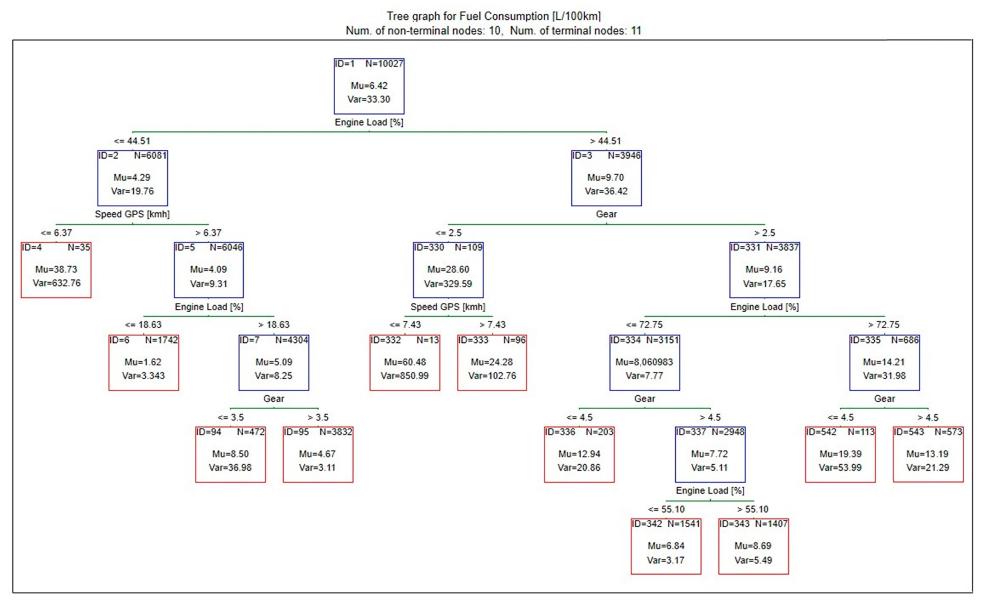
Based on the obtained results (Figure 12), it can be concluded that the highest fuel consumption occurs when the predictor values belong to leaf 332, which show the following parameters: engine load > 44.5%; gear: 1 or 2; speed < 7.5 km/h. For these parameters, the median of instantaneous fuel consumption is over 60 L/100 km.
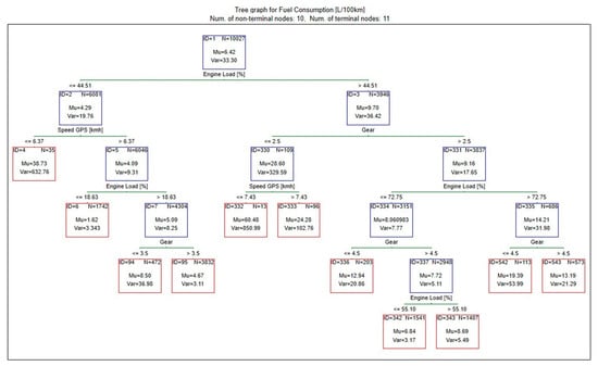
Figure 12.
Graphical diagram of created decision tree.
At the same time, a ranking of predictors that have the greatest impact on the modeled phenomenon was developed (Table 6). According to the calculations, in the analyzed model, the variables gear, speed, and engine load have the greatest influence on fuel consumption.
Table 6.
Predictor importance ranking for developed CART decision tree.
Finally, an evaluation was performed using the cross-validation method with v-value = 10. For the developed model, the errors were at the following level:
- MSE = 8.30;
- MAE = 1.36;
- MRAE = 0.22.
The second model was built using a random forest.
Before starting the analysis, the boundary settings of the presented solution were defined as follows:
- Stopping rule: percentage decrease in training error, 5%;
- Random test data proportion: 30%;
- Number of trees = 20;
- Minimum n in child node = 5;
- Maximum n of levels n = 10;
- Maximum n of nodes n = 1000.
In the next step, in order to properly assess the model’s goodness of fit, the sample was divided into two sets: training and testing. The training set was used to build the model and the test set to evaluate it.
During the construction of the model, the predictors were ranked again, indicating which had the greatest impact on the studied phenomenon (Table 7). Again, the variables engine load, speed, and gear had the greatest impact on the examined phenomenon, but in a different configuration than in the CART model.
Table 7.
Predictor importance ranking for developed random forest model.
The developed model was saved in the form of PPLM code and then implemented based on the data contained in the test sample.
The model errors were at the following level:
- MSE = 8.38;
- MAE = 1.51;
- MRAE = 0.25.
3.3. Neural Networks
Since the process of creating and teaching neural networks is experimental, it was decided to create approximately 750 networks in order to find the one with the fewest prediction errors. Input and output variables were adopted in accordance with the previous methodology.
The random sampling method was chosen with the following sizes: training sample, 80%; test sample, 10%; and validation sample, 10%. In order to force the identical learning process for each network, a fixed seed was chosen for all training networks.
MLP was chosen as the neural network due to its universality and ease of implementation. The number of hidden layers was limited to one, with 5 to 35 neurons in this layer. The activation functions used in the hidden layer were logistic, exponential, and hyperbolic tangent (tanh), and those in the output layer were identity, logistic, exponential, and tanh. Due to the large number of created neural networks, one learning algorithm was adopted, Broyden–Fletcher–Goldfarb–Shanno (BFGS), in order to allow the possibility of subsequent comparison of results. Finally, one error function was selected for all created neural networks, sum of squares (SOS).
The results of teaching neural networks can be found in Appendix A. The analysis of the results (Figure A1 and Figure A2) shows that there is no clear relationship (i.e., low correlation) between the number of neurons and the performance of the neural networks.
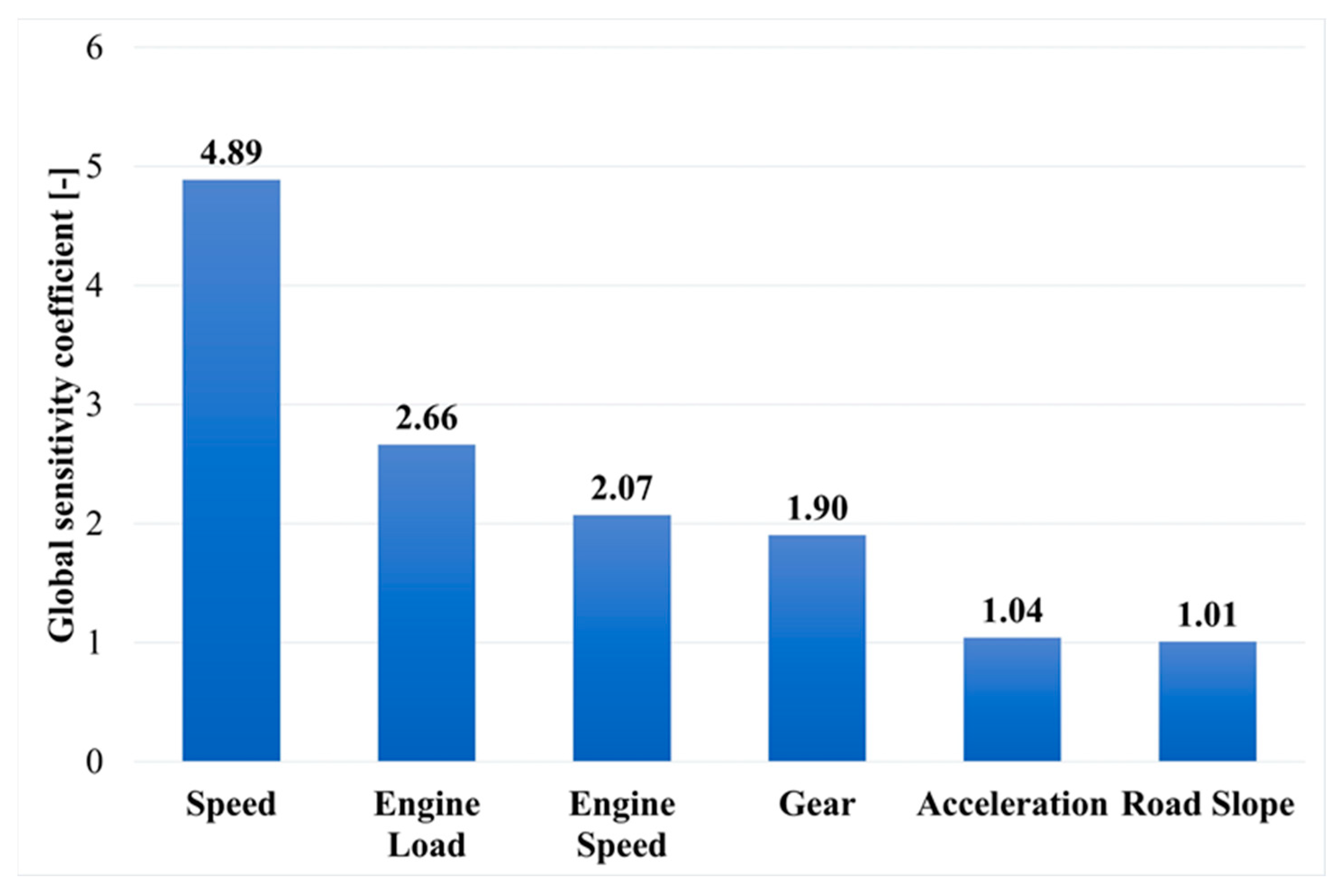
In the next stage of the analysis of the results, global sensitivity analysis was performed on 100 neural networks with the lowest error test performance values. This is a method for determining the validity of particular input variables of a neural network. For every network considered for the analysis, a coefficient for each input is calculated that describes the increase in error when the mentioned input variable is removed. If the value of the coefficient is equal to or less than 1, then the particular input variable can be removed without loss of quality of the neural network. However, if the value is greater than 1, it means that the network has a sensitivity to the variable proportional to the value. Cumulative averaged results of the global sensitivity analysis are presented In Figure 13 [43].
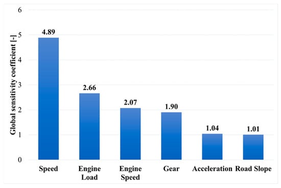
Figure 13.
Results of global sensitivity analysis of 100 selected neural networks.
The sensitivity analysis shows that the variables with the greatest impact on fuel consumption (in descending order) are speed (4.89), engine load (2.66), engine speed (2.07), and gear (1.90). Acceleration and slope (with values close to 1) can be ignored or even removed without degrading network performance.
Among all created neural network models, one model was selected with the highest testing and learning performance. Details of the parameters of the created network are as follows:
- Structure: MLP 6-35-1;
- Training data sample performance (correlation): 0.88;
- Test data sample performance (correlation): 0.89;
- Validation data sample performance (correlation): 0.86;
- Training data sample error: 3.75;
- Test data sample error: 2.76;
- Validation data sample error: 4.03;
- Activation function of hidden layer: Tanh;
- Activation function of output layer: Logistic.
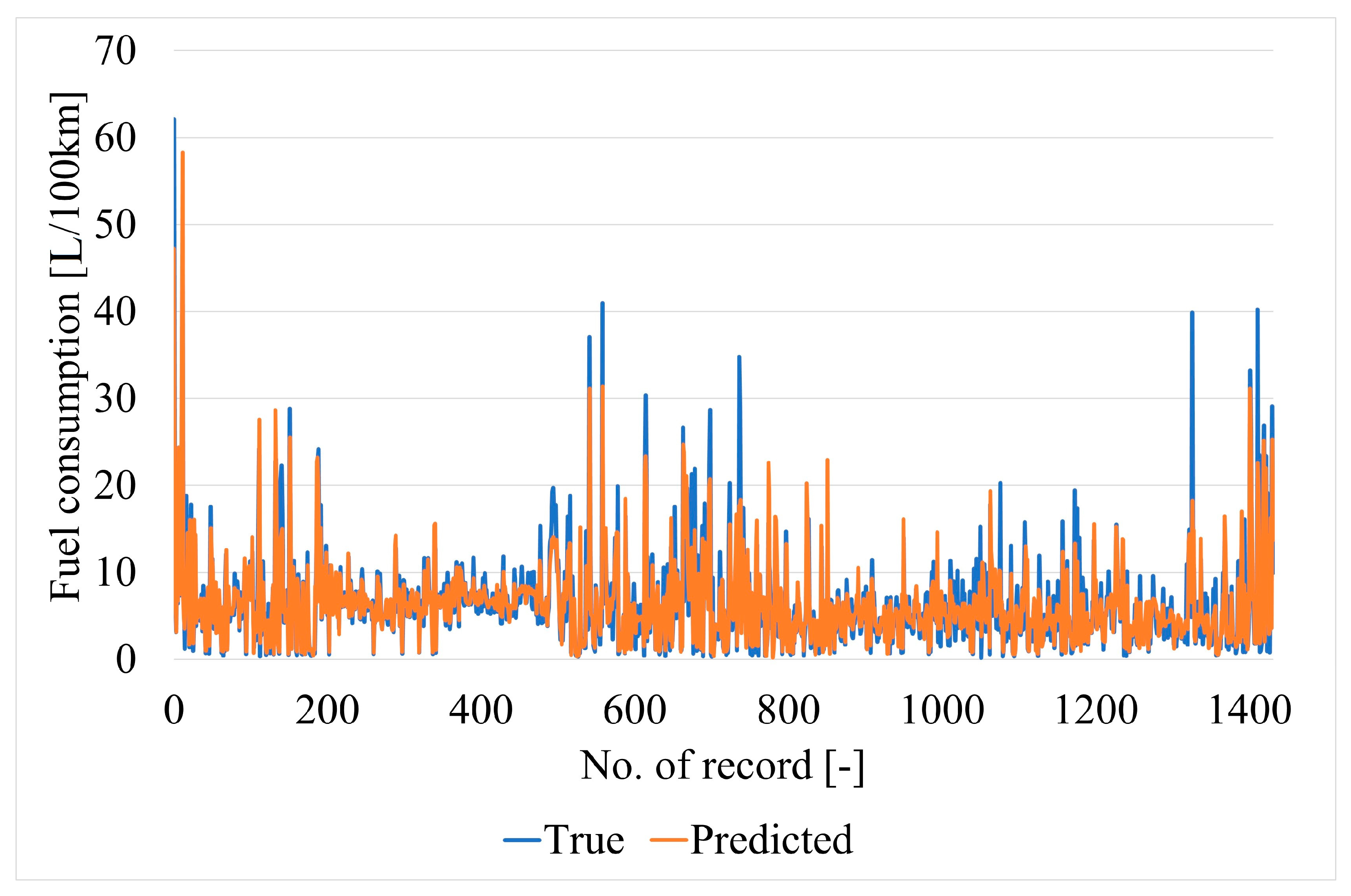
The fitting results of the chosen neural network for all data samples are shown in Figure 14. Neural network predictions and actual targets (for comparison) for the testing data samples are shown in Figure 15.
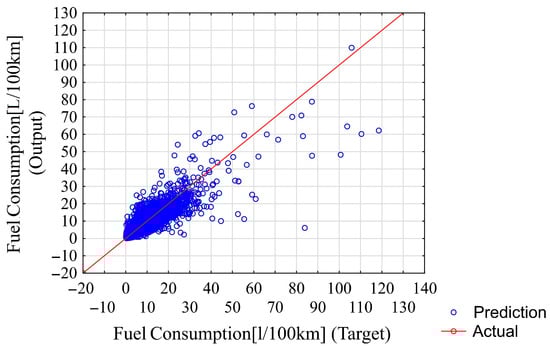
Figure 14.
Neural network predictions with respect to targets for training, validation, and testing data samples.
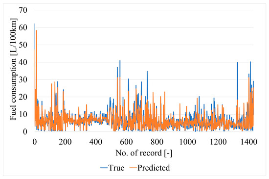
Figure 15.
Neural network predictions and true values for testing data samples.
The fitting results for the described neural network (test data samples) are as follows:
- MSE = 5.51;
- MAE = 1.37;
- MRAE = 0.30.
4. Discussion
The use of low-cost equipment reduces the possible sampling frequency, thus limiting the subsequent analysis of the collected data. The sampling frequency of the GPS modules implemented in mobile phones with the Android operating system is most often 1 Hz. In the case of the OBD-II interface, the limitations relate mainly to the hardware in terms of the bandwidth of the OBD-II module and the mobile phone (i.e., calculation capability).
The low-cost devices used in the article (OBD-II adapter, mobile phone) determine the quality of the data obtained to create fuel consumption models. The use of more expensive devices would allow for an increased amount of data (higher sampling frequency) and higher data fidelity, which in turn would allow more accurate models to be built.
In addition, the use of additional sensors, e.g., an inclinometer, which can directly measure a given parameter, in this case, the slope of the terrain, would allow for less time-consuming data processing (conversion of geographical coordinates) and possibly fewer errors.
The direction of future research could be to implement selected fuel consumption models on available embedded systems, e.g., Raspberry Pi, in order to determine their accuracy in real-time while driving a vehicle. In the case of successful verification of selected models, attempting to create a real-time decision support system for drivers could be an interesting direction.
5. Conclusions
The article presents an analysis of selected fuel consumption modeling methods and parameters that have a significant impact on the studied phenomenon. The scientific novelty of the article is in the use of low-cost technology, i.e., an OBD-II interface paired with a mobile phone, combined with modern mathematical modeling methods to create an accurate model of the fuel consumption of a vehicle that is available to every driver. The study was also carried out to develop fleet management strategies to enable transport enterprises to minimize their costs and stabilize their financial security. Nowadays, this security is threatened by inflation and sharp increases in fuel and energy prices. In order to obtain answers to the research problems, multivariate regression, a decision tree (based on the CART algorithm), and neural network models were built.
The obtained results indicate that the multivariate regression model obtained the lowest MSE, MAR, and MRSE coefficient values, which means it can be considered the best of the analyzed forecasting methods. Satisfactory forecasting error results were obtained using neural networks: an approximate 73% increase in MSE, an approximate 10% increase in MAE, and an approximate 131% increase in MRAE compared to the regression results. The worst results were achieved by the decision tree model: an approximate 163% increase in MSE, an approximate 21% increase in MAE, and an approximate 92% increase in MRAE compared to the regression results.
Implementing the developed forecasting models also allowed for an analysis of the impact of selected variables on fuel consumption. In the multivariate regression model, the phenomenon under study was most influenced by vehicle acceleration, with a 1 m/s2 increase resulting in a 0.94 increase in fuel consumption. In the decision tree model, the predictor gear, speed, and engine load had the greatest impact on the dependent variable, while engine speed and road slope had the smallest impact. In the neural network model, speed, engine load, and engine speed had the greatest impact, and acceleration and road slope had the smallest impact.
The key predictor in the most accurate multivariate regression model was acceleration, which had the least impact on the modeled phenomenon in the other two models. These differences result primarily from the different mathematical models in each method.
By using a low-cost OBD-II interface in combination with a simple multivariate regression model, it is possible to develop an operating cost management strategy (in terms of minimizing vehicle operating costs) for transport companies, without having to invest in expensive, technologically advanced TMS-class IT software, e.g., proper IT equipment.
The analysis of fuel consumption may be extended in the future by increasing the number of parameters analyzed, e.g., by including weather conditions, type of road, or vehicle technical parameters (engine, sensors, etc.). In addition, as part of future research, the authors plan to compare more mathematical methods in terms of their ability to predict fuel consumption.
Author Contributions
Conceptualization, M.R., M.G. and Ł.R.; methodology, M.R., M.G., Ł.R., D.V. and R.-M.S.; software, M.R., M.G. and Ł.R.; validation, M.R. and M.G.; formal analysis, M.R., M.G., Ł.R., D.V. and R.-M.S.; investigation, M.R., M.G., Ł.R., D.V. and R.-M.S.; resources, M.R., M.G. and Ł.R.; data curation, M.R. and Ł.R.; writing—original draft preparation, M.R., M.G., Ł.R., D.V. and R.-M.S.; writing—review and editing, M.R., M.G., Ł.R., D.V. and R.-M.S.; supervision, M.R. and M.G.; project administration, M.R.; funding acquisition, M.R. and M.G. All authors have read and agreed to the published version of the manuscript.
Funding
This research received no external funding.
Data Availability Statement
The data presented in this study are available on request from one of the corresponding authors.
Conflicts of Interest
The authors declare no conflict of interest.
Appendix A
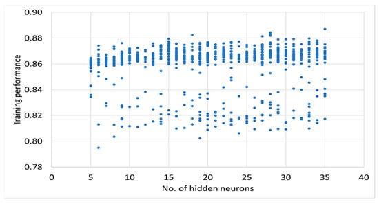
Figure A1.
Results of training performance of neural networks based on number of neurons in hidden layer.
Figure A1.
Results of training performance of neural networks based on number of neurons in hidden layer.
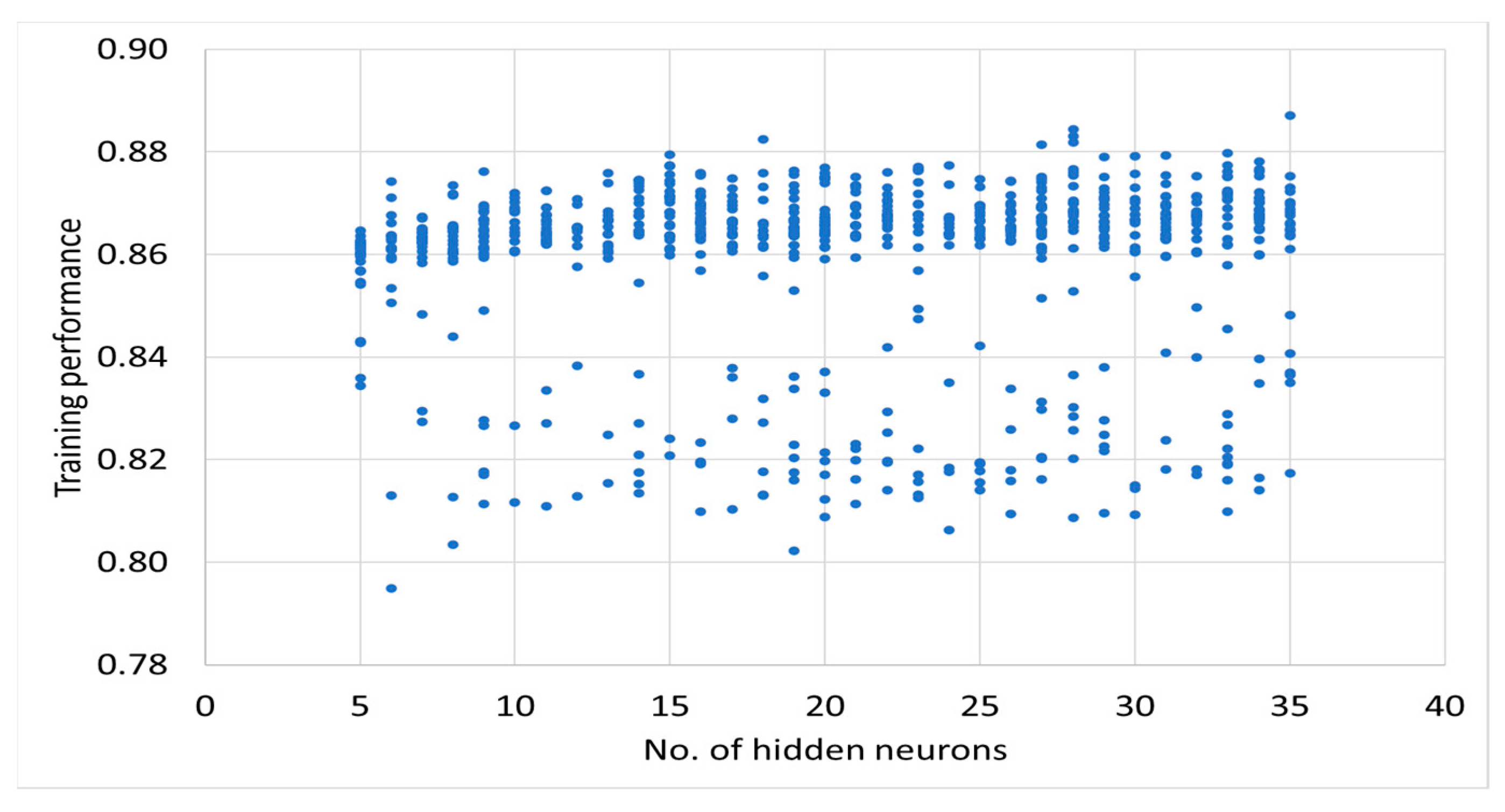
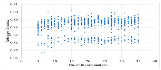
Figure A2.
The results of testing the performance of neural networks depend on the number of neurons in the hidden layer.
Figure A2.
The results of testing the performance of neural networks depend on the number of neurons in the hidden layer.

References
- Tzeiranaki, S.T.; Economidou, M.; Bertoldi, P.; Thiel, C.; Fontaras, G.; Clementi, E.L.; De Los Rios, C.F. The impact of energy efficiency and decarbonisation policies on the European road transport sector. Transp. Res. Part A Policy Pract. 2023, 170, 103623. [Google Scholar] [CrossRef]
- Shpak, N.; Podolchak, N.; Karkovska, V.; Sroka, W.; Horbal, N. The Application of Tools for Assessing the Financial Security of Enterprises. Forum Sci. Oeconomia 2022, 10, 29–44. [Google Scholar] [CrossRef]
- Ivanisevic, A.; Radisic, M.; Njegovan, M.; Pavlovic, A. Development of an Effective Planning Model for Improving Financialm Performance. Forum Sci. Oeconomia 2020, 8, 67–81. [Google Scholar] [CrossRef]
- Kilian, L.; Zhou, X. The Impact of Rising Oil Prices on U.S. Inflation and Inflation Expectations in 2020–2023. Energy Econ. 2022, 113, 106228. [Google Scholar] [CrossRef]
- Inflation, Consumer Prices (Annual %)–European Union. Available online: https://data.worldbank.org/indicator/FP.CPI.TOTL.ZG?locations=EU (accessed on 23 August 2023).
- Fuel Wholesale Prices. Available online: https://www.orlen.pl/en/for-business/fuel-wholesale-prices (accessed on 23 August 2023).
- Fuel Types of New Passenger Cars in the E.U. Available online: https://www.acea.auto/figure/fuel-types-of-new-passenger-cars-in-eu (accessed on 23 August 2023).
- Car Emissions and Global Warming. Available online: https://www.ucsusa.org/resources/car-emissions-global-warming#:~:text=Collectively%2C%20cars%20and%20trucks%20account%20for%20nearly%20one-fifth,other%20global-warming%20gases%20for%20every%20gallon%20of%20gas (accessed on 23 August 2023).
- Abukhalil, T.; AlMahafzah, H.; Alksasbeh, M.; Alqaralleh, B.A.Y. Fuel Consumption Using OBD-II and Support Vector Machine Model. J. Robot. 2020, 2020, 9450178. [Google Scholar] [CrossRef]
- Witaszek, K. Modeling of fuel consumption using artificial neural networks. Diagnostyka 2020, 21, 103–113. [Google Scholar] [CrossRef]
- Wierzbicki, S. Evaluation of the effectiveness of on-board diagnostic systems in controlling exhaust gas emissions from motor vehicles. Diagnostyka 2019, 20, 75–79. [Google Scholar] [CrossRef]
- Zervas, E. Impact of altitude on fuel consumption of a gasoline passenger car. Fuel 2011, 90, 2340–2342. [Google Scholar] [CrossRef]
- Hilgers, M. Fuel Consumption and Consumption Optimization; Springer: Berlin/Heidelberg, Germany, 2023; pp. 1–5. [Google Scholar]
- Ping, P.; Qin, W.; Xu, Y.; Miyajima, C.; Takeda, K. Impact of Driver Behavior on Fuel Consumption: Classification, Evaluation and Prediction Using Machine Learning. IEEE Access 2019, 7, 78515–78532. [Google Scholar] [CrossRef]
- Techniques for Drivers to Conserve Fuel. Available online: https://afdc.energy.gov/conserve/behavior_techniques.html (accessed on 23 August 2023).
- Puchalski, A.; Komorska, I. Driving style analysis and driver classification using OBD data of a hybrid electric vehicle. Transp. Probl. 2020, 15, 83–94. [Google Scholar]
- Lasocki, J.; Chłopek, Z.; Godlewski, T. Driving style analysis based on information from the vehicle’s OBD system. Combust. Engines 2019, 58, 173–181. [Google Scholar] [CrossRef]
- Hermawan, G.; Husni, E. Acquisition, modeling, and evaluating method of driving behavior based on OBD-II: A literature survey. In IOP Conference Series: Materials Science and Engineering; IOP Publishing: Bristol, UK, 2020; Volume 879, p. 12030. [Google Scholar]
- Alessandrini, A.; Filippi, F.; Orecchini, F.; Ortenzi, F. A new method for collecting vehicle behaviour in daily use for energy and environmental analysis. Proc. Inst. Mech. Eng. Part D J. Automob. Eng. 2006, 220, 1527–1537. [Google Scholar] [CrossRef]
- Ericsson, E. Independent driving pattern factors and their influence on fuel-use and exhaust emission factors. Transp. Res. Part D Transp. Environ. 2001, 6, 325–345. [Google Scholar] [CrossRef]
- Meseguer, J.E.; Calafate, C.T.; Cano, J.C.; Manzoni, P. DrivingStyles: A Smartphone Application to Assess Driver Behavior. In Proceedings of the 2013 IEEE Symposium on Computers and Communications (ISCC), Split, Croatia, 7–10 July 2013; pp. 535–540. [Google Scholar]
- Antosz, K.; Jasiulewicz-Kaczmarek, M.; Paśko, Ł.; Zhang, C.; Wang, S. Application of machine learning and rough set theory in lean maintenance decision support system development. Eksploat. Niezawodn. Maint. Reliab. 2021, 23, 695–708. [Google Scholar] [CrossRef]
- Ziółkowski, J.; Oszczypała, M.; Małachowski, J.; Szkutnik-Rogoż, J. Use of Artificial Neural Networks to Predict Fuel Consumption on the Basis of Technical Parameters of Vehicles. Energies 2021, 14, 2639. [Google Scholar] [CrossRef]
- Wickramanayake, S.; Dilum Bandara, H.M.N. Fuel Consumption Prediction of Fleet Vehicles Using Machine Learning: A Comparative Study. In Proceedings of the 2016 Moratuwa Engineering Research Conference (MERCon), Moratuwa, Sri Lanka, 5–6 April 2016; pp. 90–95. [Google Scholar]
- Syahputra, R. Application of neuro-fuzzy method for predictions for prediction of vehicle fuel consumption. J. Theor. Appl. Inf. Technol. 2016, 86, 138–150. [Google Scholar]
- Owczarek, P.; Brzeziński, M.; Zelkowski, J. Evaluation of light commercial vehicles operation process in a transport company using the regression modelling method. Eksploat. Niezawodn. Maint. Reliab. 2022, 24, 522–531. [Google Scholar] [CrossRef]
- Hien, N.L.H.; Kor, A.-L. Analysis and Prediction Model of Fuel Consumption and Carbon Dioxide Emissions of Light-Duty Vehicles. Appl. Sci. 2022, 12, 803. [Google Scholar] [CrossRef]
- Bifulco, G.N.; Galante, F.; Pariota, L.; Spena, M.R. A Linear Model for the Estimation of Fuel Consumption and the Impact Evaluation of Advanced Driving Assistance Systems. Sustainability 2015, 7, 14326–14343. [Google Scholar] [CrossRef]
- Zhao, D.; Li, H.; Hou, J.; Gong, P.; Zhong, Y.; He, W.; Fu, Z. A Review of the Data-Driven Prediction Method of Vehicle Fuel Consumption. Energies 2023, 16, 5258. [Google Scholar] [CrossRef]
- Abediasl, H.; Ansari, A.; Hosseini, V.; Koch, C.R.; Shahbakhti, M. Real-time vehicular fuel consumption estimation using machine learning and on-board diagnostics data. Proc. Inst. Mech. Eng. Part D J. Automob. Eng. 2023. [Google Scholar] [CrossRef]
- Rimpas, D.; Papadakis, A.; Samarakou, M. OBD-II sensor diagnostics for monitoring vehicle operation and consumption. Energy Rep. 2020, 6, 55–63. [Google Scholar] [CrossRef]
- Merkisz, J.; Rychter, M. OBD II system as a future diagnostic method of vehicles. Eksploat. Niezawodn. Maint. Reliab. 2002, 1, 38–51. [Google Scholar]
- Google Play Store—OBD Apps. Available online: https://play.google.com/store/search?q=obd&c=apps (accessed on 23 August 2023).
- Apple App Store—OBD Apps. Available online: https://www.apple.com/pl/search/obd?src=globalnav (accessed on 23 August 2023).
- Torque Pro Wiki. Available online: https://wiki.torque-bhp.com/view/Main_Page (accessed on 23 August 2023).
- Rykała, Ł.; Rubiec, A.; Przybysz, M.; Krogul, P.; Cieślik, K.; Muszyński, T.; Rykała, M. Research on the Positioning Performance of GNSS with a Low-Cost Choke Ring Antenna. Appl. Sci. 2023, 13, 1007. [Google Scholar] [CrossRef]
- OBD-II Vgate iCar Pro WIFI—Amazon.com. Available online: https://www.amazon.com/s?k=OBD-II+Vgate+iCar+Pro+WIFI&crid=3L7JBQ9IZ7R1P&sprefix=obd-ii+vgate+icar+pro+wifi%2Caps%2C210&ref=nb_sb_noss (accessed on 23 August 2023).
- Sennefelder, R.M.; Martín-Clemente, R.; González-Carvajal, R. Energy Consumption Prediction of Electric City Buses Using Multiple Linear Regression. Energies 2023, 16, 4365. [Google Scholar] [CrossRef]
- Zhang, F.; Li, D. Multiple Linear Regression-Structural Equation Modeling Based Development of the Integrated Model of Perceived Neighborhood Environment and Quality of Life of Community-Dwelling Older Adults: A Cross-Sectional Study in Nanjing, China. Int. J. Environ. Res. Public. Health 2019, 16, 4933. [Google Scholar] [CrossRef]
- Sun, J.; Dang, W.; Wang, F.; Nie, H.; Wei, X.; Li, P.; Zhang, S.; Feng, Y.; Li, F. Prediction of TOC Content in Organic-Rich Shale Using Machine Learning Algorithms: Comparative Study of Random Forest, Support Vector Machine, and XGBoost. Energies 2023, 16, 4159. [Google Scholar] [CrossRef]
- D’Cruz, J.J.M.; Alex, A.P.; Manju, V.S. Mode Choice Analysis of School Trips Using Random Forest Technique. Arch. Transp. 2022, 62, 39–48. [Google Scholar] [CrossRef]
- Tadeusiewicz, R.; Szaleniec, M. Lexicon of Neural Networks; Projekt Nauka; Fundacja na Rzecz Promocji Nauki Polskiej: Warsaw, Poland, 2015; pp. 17–133. (In Polish) [Google Scholar]
- Rykała, M.; Rykała, Ł. Economic Analysis of a Transport Company in the Aspect of Car Vehicle Operation. Sustainability 2021, 13, 427. [Google Scholar] [CrossRef]
- Osowski, S. Neural Networks for Information Processing; Oficyna Wydawnicza Politechniki Warszawskiej: Warsaw, Poland, 2006; pp. 10–100. (In Polish) [Google Scholar]
- Grzelak, M.; Rykała, M. Modeling the Price of Electric Vehicles as an Element of Promotion of Environmental Safety and Climate Neutrality: Evidence from Poland. Energies 2021, 14, 8534. [Google Scholar] [CrossRef]


Disclaimer/Publisher’s Note: The statements, opinions and data contained in all publications are solely those of the individual author(s) and contributor(s) and not of MDPI and/or the editor(s). MDPI and/or the editor(s) disclaim responsibility for any injury to people or property resulting from any ideas, methods, instructions or products referred to in the content. |
© 2023 by the authors. Licensee MDPI, Basel, Switzerland. This article is an open access article distributed under the terms and conditions of the Creative Commons Attribution (CC BY) license (https://creativecommons.org/licenses/by/4.0/).