A Low Common-Mode SVPWM for Two-Level Three-Phase Voltage Source Inverters

Abstract

In order to reduce the common-mode voltage (CMV) generated by the use of space vector pulse width modulation (SVPWM) in two-level three-phase voltage source inverters, a low common-mode SVPWM method is proposed. In this method, the voltage plane is divided into 12 sectors, and on each sector, two non-zero vectors of the same class and one single zero vector are adopted for synthesis. The action time of the zero vector is placed at both ends of each switching cycle, the currents are sampled at the beginning of each switching cycle, and the action time and sequence of vectors on each sector is provided. Simulation and experimental results show that, in the vector control system of a permanent magnet synchronous motor fed by the inverter, compared with the conventional SVPWM, the proposed method reduces the CMV peak-to-valley value by 33.333%, the CMV jump frequency by three times, and the performance of the line voltage and line current. The electromagnetic torque and rotor speed remain good, which has good application value in high-performance drives.

1. Introduction

Two-level three-phase voltage source inverters are widely used in energy conversion as a standard converter topology [1]. The space vector pulse width modulation (SVPWM) strategy, due to its high control accuracy and high voltage utilization rate, is the dominant modulation strategy for these inverters [2]. However, there are common-mode voltages (CMVs) generated by the use of SVPWM in the inverters [3]. In inverter–load systems, such as inverter–motor systems, CMVs would exacerbate negative effects such as leakage current, cable and winding insulation degradation, bearing voltage, and electromagnetic interference [4,5]. With the development of high-frequency and integrated systems, these negative effects cannot be ignored, thus requiring CMV suppression in high-performance applications [6,7].

There are two main methods for suppressing CMV: hardware methods and software methods. The former generally involve adding common-mode filters or changing the main circuit topology, while the latter generally involve improving the PWM algorithms [8,9], for example, improving the traditional sinusoidal PWM, the specified harmonic elimination PWM, the model predictive PWM, etc. [10,11,12]. In software methods, hardware costs are hardly increased and the burden of common mode filters is reduced, resulting in high cost-effectiveness and widespread attention from researchers. Due to the SVPWM strategy being the dominant modulation strategy of these inverters, improvements in conventional SVPWM have attracted much attention. At present, improved SVPWM algorithms with CMV suppression mainly include active zero-state PWM, near-state PWM, virtual vector PWM, and odd–even alternating PWM [13,14,15,16].

A typical improved SVPWM method is the active zero state PWM method proposed in ref. [13]. In the synthesis of expected vector, the two zero vectors 000 and 111 are not used, but two vectors in the opposite direction act for the same amount of time to achieve the equivalent “dynamic zero vector”. Another typical improved SVPWM method is the near-state PWM method proposed in ref. [14]. In the synthesis of the expected vector, adjacent vectors on the sector where the expected vector is located are synthesized, and a third vector on the adjacent sector is introduced to participate in the synthesis. This way, without relying on zero vectors, the unique three sets of action times can be solved to achieve the expected vector synthesis, thus avoiding the use of zero vectors. Ref. [15] proposes a virtual vector PWM method. Using two adjacent non-zero fundamental vectors to synthesize a virtual vector, a total of six virtual vectors were obtained. With six virtual vectors as boundaries, the voltage α-β plane is divided into six sectors. On each sector, two virtual vectors and two non-zero fundamental vectors in opposite directions are used for synthesis. Ref. [16] researches an odd even-alternating PWM method. The voltage α-β plane is divided into six sectors, which differ in position by 30° compared to the six sectors of the conventional SVPWM. Only three non-parity active vectors are used for synthesis on odd-numbered sectors, and only three parity active vectors are used for synthesis on even-numbered sectors.

The common feature of the above methods is that the zero vectors are not used, and instead, the synthesis of other non-zero vectors are used to replace the zero vectors. These methods can reduce the CMV amplitude to U_d/6 (U_d is the DC link voltage value of the inverter) because the CMV amplitude under zero vector action is equal to U_d/2, while that under non-zero vector action is equal to U_d/6. However, due to the fact that the vectors involved in the synthesis are all non-zero vectors, the harmonics of the inverter output line voltage increase, resulting in a decrease in other performances of the system, generally lower than the conventional SVPWM [17,18]. In addition, the closed-loop current regulation of the inverter system usually requires sensors to directly measure the output line currents. Current sampling should be carried out in the middle of the zero-vector segment, and the instantaneous value of the sampled current at this point closes to the fundamental value of the inverter output current. However, the current sampling of the above methods is carried out under the action of a non-zero vector, resulting in a significant difference between the sampling value and the fundamental value. The harmonics of the current feedback value increase, further reducing the other performances of the system [19,20].

From this, it can be seen that the improved SVPWM algorithms suppress the CMV by discarding zero vectors, but the performance of line voltage and line current deteriorates. The conventional SVPWM algorithm achieves excellent line voltage and line current performance by using two types of zero vectors, but the CMV performance is relatively poor. The CMV and the line voltage are conflicting performance criteria [21,22]. In order to reduce the CMV of the inverter system while not deteriorating other performances of the system, this paper proposes a low common-mode SVPWM method, which combines two non-zero vectors of the same type and one single zero vector. Simulation and experimental verification are conducted in the vector control system of a permanent magnet synchronous motor (PMSM) fed by the inverter. The proposed method can reduce the peak-valley value, jump the frequency of the CMV, and maintain good line voltage, line current, torque, and speed.

2. Low Common-Mode SVPWM Method

2.1. Classification of Basic Vectors

The inverter using SVPWM is a three-phase power supply, and the sum of its three phase voltages may not necessarily be equal to zero. The arithmetic mean of the three phase voltages is defined as the common-mode voltage. In the inverter–motor system, the potential difference between the star node of the motor stator winding and the midpoint of the inverter DC link is equal to the CMV, as shown in Figure 1.

The inverter has 8 switch states, corresponding to 8 basic vectors, which are divided into four categories according to different CMV values, as shown in

Table 1. Classification of basic vectors.

Classes	Basic Vectors	SA	SB	SC	CMV Values
Class (i)	V0	0	0	0	−Ud/2
	V1	1	0	0
Class (ii)	V3	0	1	0	−Ud/6
	V5	0	0	1
	V2	1	1	0
Class (iii)	V4	0	1	1	Ud/6
	V6	1	0	1
Class (iv)	V7	1	1	1	Ud/2

. In this table, S_k (k = A, B, C) is the switching function, defined as:

$${\mathrm{S}}_k=\{\begin{array}{l}1 k-\mathrm{phase} \mathrm{upper} \mathrm{bridge} \mathrm{arm} \mathrm{conduction}, \mathrm{lower} \mathrm{bridge} \mathrm{arm} \mathrm{disconnection}\\ 0 k-\mathrm{phase} \mathrm{lower} \mathrm{bridge} \mathrm{arm} \mathrm{conduction}, \mathrm{upper} \mathrm{bridge} \mathrm{arm} \mathrm{disconnection}\end{array}$$

From Table 1, it can be seen that the basic vectors of class (i) and class (iv) are zero vectors V₀ and V₇, and the CMV amplitude can reach U_d/2. The basic vectors of class (ii) and class (iii) are non-zero vectors, with a CMV amplitude of U_d/6.

The conventional SVPWM uses two zero vectors, V₀ and V₇, so the CMV valley value is −U_d/2, the peak value is U_d/2, and the peak-valley value is U_d. The low common-mode SVPWM proposed in this article only uses a zero vector (using V₀ as an example), so the CMV valley value is −U_d/2, the peak value is U_d/6, and the peak-valley value is 2U_d/3, which is 33.333% lower than the conventional SVPWM.

2.2. Synthesis of Expected Vectors

In the conventional SVPWM, the voltage α-β plane is divided into six sectors, S1 to S6, as shown in Figure 2a. Six non-zero vectors are used as boundaries, and the expected vector is synthesized on each sector using the sector start edge vector, sector end edge vector, and two classes of zero vectors. The maximum length of the expected vector is equal to the radius of the incircle of the regular hexagon in Figure 2a [23].

Here, we divide each sector in Figure 2a into two sectors, resulting in 12 sectors numbered S1′ to S12′, as shown in Figure 2b. On each sector, the expected vector is synthesized using the zero vector V₀ and two non-zero vectors of the same class. For example, on sector S1′, the zero vector V₀, the vector V₁ at the beginning of the sector, and the vector V₃ of the same class outside the sector are synthesized, as shown in Figure 3a. Due to the fact that the V₁ and V₃ are vectors of the same class and have the same CMV value, the CMV can be kept constant, thereby reducing the CMV jump frequency. Similarly, on sector S2′, the zero vector V₀, the vector V₂ at the end of the sector, and the vector V₆ of the same class outside the sector are synthesized, as shown in Figure 3b.

The calculation formula for the action times of the three vectors on each sector are as follows:

On sector S1′, the action times of V₁, V₃, and V₀ within a switching cycle T_s are recorded as T₁, T₃, and T₀, respectively. Then, there is a volt second balance equation:

$$\{\begin{array}{l}{T}_1{V}_1+T_3{V}_3+T_0{V}_0=T_{\mathrm{s}}{V}_{\mathrm{ref}}\\ T_1+T_3+T_0=T_{\mathrm{s}}\end{array}$$

(1)

in which V_ref is the expected vector.

After (1) is solved, the result is as follows:

$$\{\begin{array}{l}{T}_1=\frac{2}{\sqrt{3}}\frac{V_{\mathrm{ref}}}{V}\sin \left({120}^{°}-\theta \right)·T_{\mathrm{s}}\\ T_3=\frac{2}{\sqrt{3}}\frac{V_{\mathrm{ref}}}{V}\sin \theta ·T_{\mathrm{s}}\\ T_0=T_{\mathrm{s}}-T_1-T_3\end{array}$$

(2)

in which V_ref is the length of the expected vector; θ is the angle between the expected vector and the beginning edge of the sector, 0° ≤ θ ≤ 30°; and V is the length of the non-zero vector.

The action times of the basic vectors on sectors S3′, S5′, S7′, S9′, and S11′ are similar to (2).

On sector S2′, the action times of V₂, V₆, and V₀ within a switching cycle T_s are recorded as T₂, T₆, and T₀, respectively, then there is a volt second balance equation:

$$\{\begin{array}{l}{T}_2{V}_2+T_6{V}_6+T_0{V}_0=T_{\mathrm{s}}{V}_{\mathrm{ref}}\\ T_2+T_6+T_0=T_{\mathrm{s}}\end{array}$$

(3)

After (3) is solved, the result is as follows:

$$\{\begin{array}{l}{T}_2=\frac{2}{\sqrt{3}}\frac{V_{\mathrm{ref}}}{V}\sin \left(\theta +{90}^{°}\right)·T_{\mathrm{s}}\\ T_6=\frac{2}{\sqrt{3}}\frac{V_{\mathrm{ref}}}{V}\sin \left[{120}^{°}-\left(\theta +{90}^{°}\right)\right]·T_{\mathrm{s}}\\ T_0=T_{\mathrm{s}}-T_2-T_6\end{array}$$

(4)

The action times of the basic vectors on sectors S4′, S6′, S8′, S10′, and S12′ are similar to (4).

The basic vectors on each sector and their action times are shown in

Table 2. Basic vectors on each sector and their action times.

Sectors	Basic Vectors	Action Time	Sectors	Basic Vectors	Action Time
S1′	V0 V1 V3	Equation (2)	S7′	V0 V4 V6	Similar to (2)
S2′	V0 V2 V6	Equation (4)	S8′	V0 V3 V5	Similar to (4)
S3′	V0 V2 V4	Similar to (2)	S9′	V0 V1 V5	Similar to (2)
S4′	V0 V1 V3	Similar to (4)	S10′	V0 V4 V6	Similar to (4)
S5′	V0 V3 V5	Similar to (2)	S11′	V0 V2 V6	Similar to (2)
S6′	V0 V2 V4	Similar to (4)	S12′	V0 V1 V5	Similar to (4)

. According to the above synthesis method, the maximum length of the expected vector is equal to the radius of the inscribed circle of the regular hexagram in Figure 2b.

2.3. Sequences of Basic Vectors

There are three vectors at work during each switching cycle on each sector, and the number of sequences of these three vectors is 6 (that is, 3! = 6). Taking sector S2′ as an example, the six sequences are shown in

Table 3. Sequences of basic vectors (taking sector S2′ as an example).

Sequence Number	Sequences of Basic Vectors within One Switching Cycle	Number of Switches	Current Sampling Synchronized with Zero Vector
sequence 1	V0V6V2V2V6V0	8	convenient
sequence 2	V0V2V6V6V2V0	8	convenient
sequence 3	V6V2V0V0V2V6	8	convenient
sequence 4	V2V6V0V0V6V2	8	convenient
sequence 5	V6V0V2V2V0V6	8	inconvenient
sequence 6	V2V0V6V6V0V2	8	inconvenient

. In order to ensure the symmetry of the SVPWM output waveform, in Table 3, the first half of the switching cycle is a positive sequence, and the second half is an inverse sequence.

As mentioned in the introduction, in the inverter–motor system, current sampling should be carried out in the middle of the zero-vector segment, and the instantaneous value of the sampled current at this point should be close to the fundamental value of the inverter output current. Sequence 5 and sequence 6 in Table 3 are difficult to achieve in current sampling, so these two sequences are not adopted.

For the remaining four sequences, the number of switches within one switching cycle is 8. However, further analyses show that sequences 3 and 4 switch during sector transition, while sequences 1 and 2 do not have this problem. Therefore, sequences 1 and 2 are adopted. In order to balance the number of switches of power semiconductor devices, sequence 1 may be used in the first half of each sector, and sequence 2 may be used in the second half of each sector.

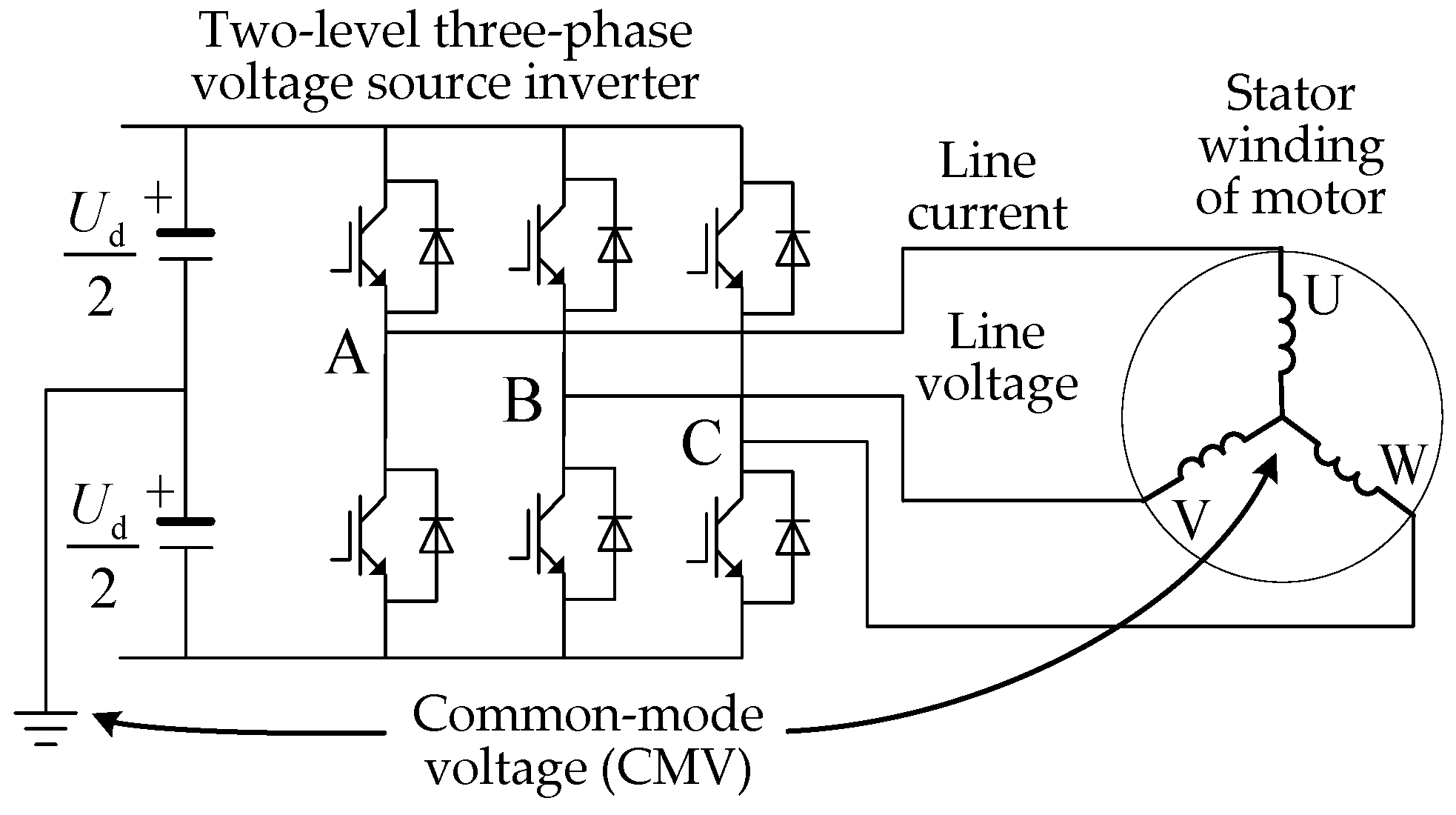
2.4. Waveform of Common-Mode Voltages

Figure 4 shows the CMV waveforms of the conventional SVPWM and the low common-mode SVPWM in 12 sectors. For simplicity, on each sector, only the CMV waveform during one switching cycle is drawn, while the CMV waveforms during other switching cycles are similar.

Comparing Figure 4a,b, it can be seen that the CMV peak value of the conventional SVPWM is U_d/2, the valley value is −U_d/2, and the peak-valley value is U_d. The CMV peak value of the low common-mode SVPWM is U_d/6, the valley value is −U_d/2, and the peak-valley value is 2U_d/3, a decrease of 33.33%. The conventional SVPWM results in the CMV value jumping 6 times within a switching cycle; therefore, the jumping frequency is equal to 6 times the switching frequency. However, the low common-mode SVPWM only jumps twice within a switching cycle, resulting in a jumping frequency equal to twice the switching frequency, which is reduced by three times. The smaller the CMV peak-valley value and jumping frequency, the smaller the negative impact on the inverter–motor system.

The above theoretical design indicates that the proposed low common-mode SVPWM has a CMV suppression effect and does not abandon zero vectors; therefore, it would maintain good line voltage and line current performance. We further validate this using simulations and experiments.

3. Simulation and Experimental Results

On the vector control system platform of a PMSM with a rotor flux orientation and stator excitation current i_d = 0, simulations and experiments were conducted for two methods: the conventional SVPWM and the low common-mode SVPWM. The relevant results were compared to verify their effectiveness. The simulation parameters are consistent with the experimental device parameters, which are shown in

Table 4. Simulation and experimental parameters.

Parameters	Values	Parameters	Values
Inverter DC link voltage	311 V	Motor stator resistance	0.958 Ω
Inverter switching frequency	5 kHz	Motor stator d-axis inductance	0.00525 H
Line current sampling frequency	5 kHz	Motor stator q-axis inductance	0.012 H
Speed command value	750 r/min	Motor rotor flux linkage	0.1827 W
Motor-rated voltage	130 V/50 Hz	Motor damping coefficient	0.008 N·m·s
Motor moment of inertia	0.003 kg·m2	Motor number of pole pairs	4

.

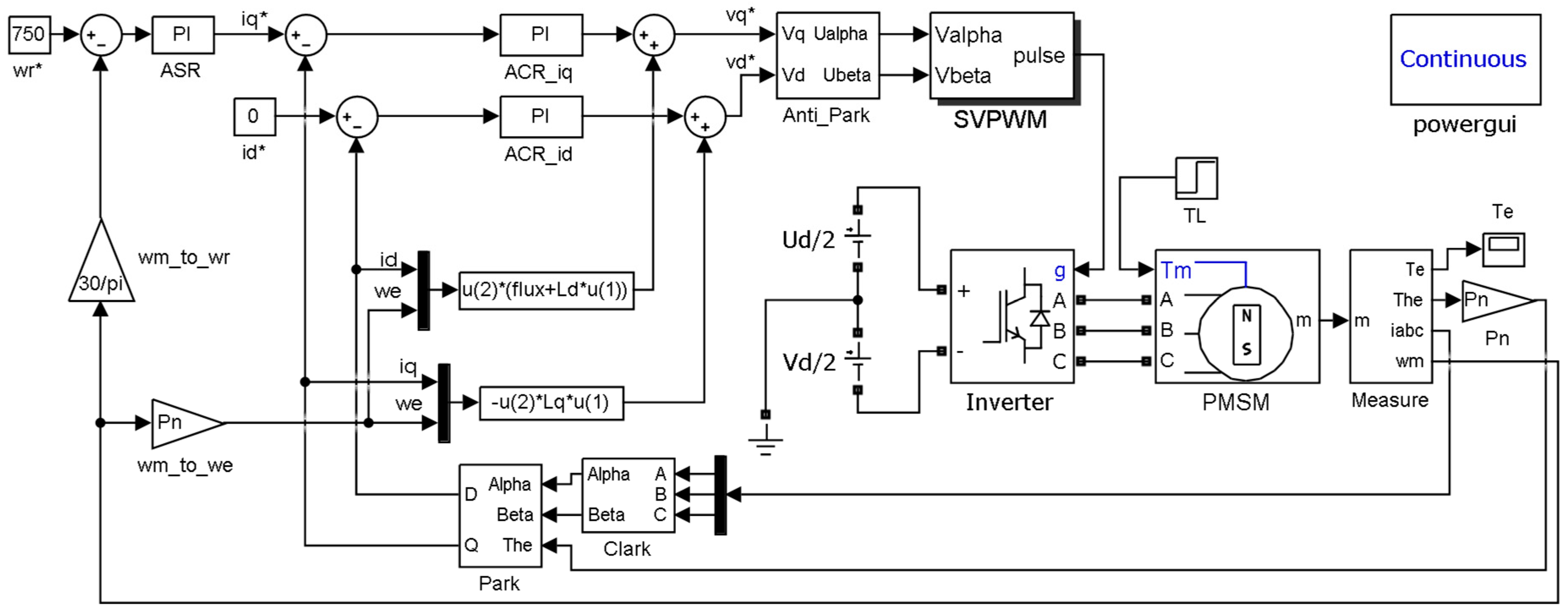
3.1. Simulation Results

The simulation is executed using MATLAB R2016a software, and the simulation model is shown in Figure 5.

The simulations start with no load. A load torque of 10 N·m is applied at 0.2 s, and it stops at 0.4 s. The CMV simulation waveforms and the fast Fourier transform (FFT) analyses of the two methods are shown in Figure 6.

Comparing Figure 6a,b, it can be seen that the CMV peak value and valley value for conventional SVPWM are 155.5 V and −155.5 V, while for the low common-mode SVPWM, they are 51.83 V and −155.5 V. Comparing Figure 6c,d, it can be seen that the CMV of the conventional SVPWM jumps six times within a switching cycle, while the CMV of the low common-mode SVPWM only jumps two times. Therefore, the peak-valley value of the latter is reduced by 33.333% compared to the former, and the jumping frequency is reduced by three times compared to the former, all of which are consistent with the theoretical analysis results.

Comparing Figure 6e,f, it can be seen that the CMV fundamental (50 Hz) amplitudes in the two methods are 0.07931 V and 0.1874 V, respectively, which are close to zero, indicating that neither CMV contains the fundamental frequency component. The total harmonic distortion (THD) for the CMV does not provide meaningful results due to a very small fundamental amplitude. The CMV harmonics are mainly at the switching frequency harmonics, which amounts to 168.8 V in the conventional SVPWM and only 96 V in the low common-mode SVPWM, a decrease of 43.13%. Additionally, due to the use of one zero vector in the low common-mode SVPWM, the CMV has a certain DC component.

The simulation waveforms of the line voltage u_AB after loading in the two methods, their FFT analysis, and their waveforms obtained through low-pass filtering (LPF) are shown in Figure 7.

From Figure 7a,b, it can be seen that the peak value and valley value of the line voltage for both methods are 311 V and −311 V, respectively, which is consistent with the theoretical analysis. Although Figure 7a,b shows that the line voltage waveforms of the two methods are different, it can be seen from Figure 7c,d that the fundamental amplitude of the line voltage of both methods is equal to 130.8 V, which is consistent with the theoretical value of 130 V.

From Figure 7c,d, it can be seen that the THD for the line voltage in the low common-mode SVPWM is slightly higher than that in the conventional SVPWM. This is because the conventional SVPWM uses two zero vectors, while the low common-mode SVPWM uses single zero vector, which increases the high-frequency harmonic component of the line voltage. The line voltage harmonics in the conventional SVPWM are mainly two times the switching frequency harmonics, with an amplitude of 100 V. However, the low common-mode SVPWM mainly has harmonics of one times the switching frequency, with an amplitude of only 87 V.

Upon comparison of Figure 7e,f, we find the waveforms obtained through LPF in the two methods are substantially the same, both of which are sine waves with an amplitude of 130.8 V. Overall, the line voltage quality in the low common-mode SVPWM is comparable to that of the conventional SVPWM.

Under the excitation of the line voltages, the simulation waveforms of the line current i_A and their FFT analysis in the two methods are shown in Figure 8.

A comparison of Figure 8a,b shows that the no-load and load waveforms, as well as the transient-state and steady-state waveforms of line current in the two methods, are nearly identical. Inspection of Figure 8c,d indicates that the two line currents after loading are a sine wave with an amplitude of 9.6 A. Further reference to Figure 8e,f indicates that the fundamental amplitudes of the two line currents after loading are 9.597 A and 9.587 A, respectively, which are nearly identical.

From Figure 8e,f it can be seen that the line current harmonics in the conventional SVPWM are mainly two times the switching frequency harmonics, with an amplitude of 0.11 A, while in the low common-mode SVPWM, they are mainly a harmonic of one times the switching frequency, with an amplitude of 0.23 A. Overall, the line current quality of the low common-mode SVPWM is comparable to that of the conventional SVPWM.

The simulation results of the electromagnetic torque and rotor speed of the PMSM using the two methods are shown in Figure 9.

Inspection of Figure 9a,b indicates that the torque response in the two methods is nearly identical; that is, the no-load and load values, transient-state, and steady-state waveforms are almost identical. From Figure 9c,d, it can be seen that the speed response in the two methods is also nearly identical.

The above simulation results indicate that the low common-mode SVPWM can effectively suppress the peak-valley value and the jump frequency of the CMV, while the performance of the line voltage, line current, torque, and speed does not decrease, which is equivalent to the conventional SVPWM.

3.2. Experimental Results

During the experiment, the inverter–motor system was started with no load, and a load of 10 N·m was applied at 20 s. The experimental setup is shown in Figure 10. The waveforms of CMV, line voltage through LPF, line current, torque, and speed for the two methods are shown in Figure 11.

Figure 11a,b shows the CMVs in the two methods, with peak-valley values consistent with the theoretical analysis and simulation results. The CMV peak-valley values in the low common-mode SVPWM are reduced by 33.333% compared to the conventional SVPWM, thus reducing the negative impact on the inverter–motor system.

Figure 11c,d show the locally enlarged CMVs in the two methods. It can be seen that the CMV of the conventional SVPWM jumps six times in a switching cycle, while the CMV of the low common-mode SVPWM jumps only two times. The jumping frequency of the low common-mode SVPWM is three times lower than that of the conventional SVPWM, thus reducing the negative impact on the inverter–motor system.

Figure 11e,f shows the line voltages u_AB and u_BC through the LPF before and after loading in the two methods. The comparison shows that the line voltage quality of the two methods is equivalent. Figure 11g,h shows the line currents i_A and i_B before and after loading in the two methods. The comparison shows that the line current qualities of the two methods are also equivalent.

Figure 11i,j shows the electromagnetic torque and rotor speed before and after loading in the two methods. The adjustment time and overshoot during the transition process are nearly identical, and the steady-state response is also nearly identical.

The above experimental results are consistent with the theoretical analysis and simulation results, thus further demonstrating that the low common-mode SVPWM has a CMV suppression effect while maintaining good other system performance, which is substantially the same as the conventional SVPWM.

The above experimental results were obtained under rated operating conditions. In order to verify the CMV suppression effect of the low common-mode SVPWM under non-rated operating conditions, three critical operating condition experiments were conducted.

In critical condition 1, the speed command value was 75 r/min, the inverter–motor system was started with no load, and a load of 10 N·m was applied at 20 s. When the load was applied, the speed dynamically dropped to zero and then recovered to 75 r/min; therefore, this was a critical operating condition.

In critical condition 2, the speed command value was 1050 r/min, the inverter–motor system was started with no load, and a load of 10 N·m was applied at 20 s. When the load was applied, the length of the expected vector was 177 V, which was close to the maximum length of 179 V within the linear modulation range. Therefore, this was a critical operating condition.

In critical condition 3, the speed command value was 750 r/min, the inverter–motor system was started with no load, and a load of 20 N·m was applied at 20 s. When the load was applied, the length of the expected vector was 178 V, which was close to the maximum length of 179 V within the linear modulation range. Therefore, this was also a critical operating condition.

The locally enlarged CMVs under the three critical operating conditions mentioned above are shown in Figure 12.

From Figure 12, it can be seen that the peak value, valley value, and jumping frequency of the CMV waveforms under the three critical operating conditions were consistent with the rated operating conditions, with the difference being that the CMV duty cycle was different. The CMV duty cycle of critical condition 1 was less than that of the rated condition, while the CMV duty cycles of critical conditions 2 and 3 were greater than that of the rated condition. Therefore, the proposed low common-mode SVPWM could also effectively reduce the CMV under the critical operating conditions.

In addition, we simulated open-circuit or short-circuit faults in the bridge arm of the inverter, open-circuit or short-circuit faults in the stator winding of the motor, and open-circuit faults in the sensors in the experimental device. The results showed that if the proposed low common-mode SVPWM method was still used after the fault occurred, the peak value or valley value of the tested CMVs would increase, and the CMV jumping frequency would change. Therefore, the proposed method was not suitable for operation under the fault conditions.

4. Discussion

This section provides a discussion of the CMVs of the eight SVPWM methods, including the proposed conventional SVPWM and the low common-mode SVPWM. The eight methods are the conventional SVPWM, the discontinuous PWM with maximum clamping (DPWMmax), the discontinuous PWM with minimum clamping (DPWMmin) [1,2,3], active zero-state PWM [13], near-state PWM [14], virtual vector PWM [15], odd–even alternating PWM [16], and the low common mode PWM proposed in this paper. The waveforms of the switching functions and CMVs of the eight methods within one switching cycle are shown in Figure 13.

From Figure 13, it can be seen that the peak value, valley value, and jumping frequency of the CMVs for the eight methods are different. For the purposes of comparison and analysis,

Table 5. Features of the eight SVPWM methods.

Method Number	SVPWM Method	CMV Peak Value	CMV Valley Value	Number of CMV Jumps in a Period	Number of Switches in a Period	Whether to Use Zero Vector	Line Voltage Quality	Current Sampling Quality
1	Conventional SVPWM	Ud/2	−Ud/2	6	6	Yes	Excellent	Excellent
2	DPWMmax	Ud/2	−Ud/6	4	4	Yes	Good	Good
3	DPWMmin	Ud/6	−Ud/2	4	4	Yes	Good	Good
4	Active zero-state PWM	Ud/6	−Ud/6	6	6	No	Medium	Medium
5	Near-state PWM	Ud/6	−Ud/6	4	4	No	Medium	Medium
6	Virtual vector PWM	Ud/6	−Ud/6	6	6	No	Medium	Medium
7	Odd–even alternating PWM	−Ud/6	−Ud/6	0	8	No	Medium	Medium
8	Low common-mode SVPWM	Ud/6	−Ud/2	2	6 or 8	Yes	Good	Good

provides a summary of some characteristics of the eight methods.

Analyzing Table 5, it can be seen that the CMV peak-valley value of method 1, namely the conventional SVPWM, is U_d, and the number of CMV jumps within a switching period is six. The two indicators are the largest among the eight methods, which indicate that the CMV performance of this method is relatively poor. However, its line voltage and line current quality are excellent, which are the best among the eight methods because it uses two zero vectors.

Method 2 and method 3 are discontinuous PWMs, with a CMV peak-valley value of 2U_d/3, which is 33.333% lower than the conventional SVPWM. The number of CMV jumps within a switching period is four, which is reduced by 33.333% compared to the conventional SVPWM. Their line voltage and line current quality are good but slightly inferior to the conventional SVPWM because they use one vector instead of two zero vectors.

The common feature of methods 4 to 7 is that they do not use zero vectors; therefore, their performance in line voltage and line current quality is mid-level. The CMV peak-valley values for methods 4, 5, and 6 are U_d/3, which is 66.667% lower than the conventional SVPWM. The number of CMV jumps within a switching period is six or four. It is worth pointing out that the CMV of method 7 remains unchanged at −U_d/6 in a switching period and −U_d/6 in a fundamental period, which makes it the best among the eight methods in terms of CMV performance. However, it has eight switching actions, which is the highest among the eight methods, and the performance of the line voltage and line current quality is mid-level.

Method 8, the low common-mode SVPWM proposed in this paper, achieves effective compromise optimization between CMV performance and line voltage performance, which not only has the effect of suppressing CMV, but also has good line voltage performance. The CMV peak-valley value is 2U_d/3, which is reduced by 33.333% compared to the conventional SVPWM. The number of CMV jumps within a switching period is two, which is three times lower than the conventional SVPWM. Due to using a zero vector, the performances of the line voltage and line current quality are good.

5. Conclusions

The CMV and line voltage are conflicting performance criteria in two-level three-phase voltage source inverters. The low common-mode SVPWM proposed in this paper achieves effective compromise optimization between CMV performance and line voltage performance. It has both CMV suppression and good line voltage performance.

The low common-mode SVPWM combines one single zero vector and two non-zero vectors of the same class. Compared with the conventional SVPWM, the proposed method reduces the CMV peak-to-valley value by 33.333% and the CMV jumping frequency by three times. Therefore, it has a good CMV suppression effect. At the same time, the performance of the line voltage, line current, electromagnetic torque, and rotor speed remains good. This method has good engineering reference applications value in inverter systems, with high requirements for electromagnetic compatibility and interference. In the future, we will conduct in-depth research on the nonlinear compensation and overmodulation techniques of the low common-mode SVPWM.

References

1. Mirafzal, B. Power Electronics in Energy Conversion Systems; McGraw-Hill Education: New York, NY, USA, 2022; pp. 206–210. ISBN 978-1-260-46380-4. [Google Scholar]
2. Suntio, T.; Messo, T. Power Electronics in Renewable Energy Systems; MDPI: Basel, Switzerland, 2019; pp. 1–8. ISBN 978-3-03921-045-9. [Google Scholar]
3. Geyer, T. Model Predictive Control of High Power Converters and Industrial Drives; John Wiley & Sons: Hoboken, NJ, USA, 2017; pp. 77–84. ISBN 978-1-119-01090-6. [Google Scholar]
4. Fan, L.; Liu, Z.; Liang, Y.; Li, H.; Rao, B.; Yin, S.; Jiang, D. Analysis and utilization of common-mode voltage in inverters for power supply. IEEE Trans. Power Electron. 2023, 7, 8811–8824. [Google Scholar] [CrossRef]
5. Luo, Q.; Zheng, J.; Sun, Y.; Yang, L. Optimal modeled six-phase space vector pulse width modulation method for stator voltage harmonic suppression. Energies 2018, 18, 2598. [Google Scholar] [CrossRef]
6. Abu-Rub, H.; Malinowski, M.; Al-Haddad, K. Power Electronics for Renewable Energy Systems, Transportation and Industrial Applications; John Wiley & Sons: Hoboken, NJ, USA, 2014; pp. 664–671. ISBN 978-1-118-63403-5. [Google Scholar]
7. Zheng, J.; Rong, F.; Li, P.; Huan, S.; He, Y. Six-phase SVPWM with common-mode voltage suppression. IET Power Electron. 2018, 15, 2461–2469. [Google Scholar] [CrossRef]
8. Sudhoff, S.D. Power Magnetic Devices: A Multi-Objective Design Approaches, 2nd ed.; John Wiley & Sons: Hoboken, NJ, USA, 2022; pp. 543–572. ISBN 978-1-119-67465-8. [Google Scholar]
9. Wu, B.; Narimni, M. High-Power Converters and AC Drives, 2nd ed.; John Wiley & Sons: Hoboken, NJ, USA, 2017; pp. 101–109. ISBN 978-1-119-15603-1. [Google Scholar]
10. Tan, B.; Gu, Z.; Shen, K.; Ding, X. Third harmonic injection SPWM method based on alternating carrier polarity to suppress the common mode voltage. IEEE Access 2019, 7, 9805–9816. [Google Scholar] [CrossRef]
11. Dai, J.; Li, G.; Hu, C. Study on a new method to eliminate the common-mode voltage based on improved SHEPWM. IEEE Conf. Ind. Electron. Appl. 2015, 1633–1636. [Google Scholar]
12. Guo, L.; Jin, N.; Gan, C.; Luo, K. Hybrid voltage vector preselection-based model predictive control for two-level voltage source inverters to reduce the common-mode voltage. IEEE Trans. Ind. Electron. 2020, 6, 4680–4691. [Google Scholar] [CrossRef]
13. Cetin, N.O.; Hava, A.M. Interaction between the filter and PWM units in the sine filter configuration utilizing three-phase AC motor drives employing PWM inverters. In Proceedings of the IEEE Energy Conversion Congress & Exposition, Atlanta, GA, USA, 12–16 September 2010; pp. 2592–2599. [Google Scholar]
14. Ün, E.; Hava, A.M. A near-state PWM method with reduced switching losses and reduced common-mode voltage for three-phase voltage source inverters. IEEE Trans. Ind. Appl. 2009, 2, 782–793. [Google Scholar] [CrossRef]
15. Tian, K.; Wang, J.; Wu, B.; Xu, D.; Cheng, Z.; Zargari, N.R. A virtual space vector modulation technique for the reduction of common-mode voltages in both magnitude and third-order component. IEEE Trans. Power Electron. 2016, 1, 839–848. [Google Scholar] [CrossRef]
16. Zheng, J.; Lyu, M.; Li, S.; Luo, Q.; Huang, K. Common-mode reduction SVPWM for three-phase motor fed by two-level voltage source inverter. Energies. 2020, 12, 3884. [Google Scholar] [CrossRef]
17. Lee, J.; Park, J. Selection of PWM methods for common-mode voltage and DC-link capacitor current reduction of three-phase VSI. IEEE Trans. Ind. Appl. 2023, 1, 1064–1076. [Google Scholar] [CrossRef]
18. Singh, H.; Sudhoff, S.D. A common-mode shorting network to reduce common-mode excitation of three-phase two-level electric drives. IEEE Open Access J. Power Energy 2023, 10, 14–24. [Google Scholar] [CrossRef]
19. Jiang, D.; Shen, Z.; Liu, Z.; Hun, X.; Wang, Q.; He, Z. Progress in active mitigation technologies of power electronics noise for electrical propulsion system. Proc. CSEE 2020, 16, 5291–5301. [Google Scholar]
20. Zhao, R.; Jiang, X.; Wang, C.; Wang, Y.; Xu, H.; Yan, Q. A novel zero-sequence-voltage-balanced SVPWM with the analyses of common-mode voltage and differential-mode current. IEEE J. Emerg. Sel. Top. Power Electron. 2022, 10, 2483–2496. [Google Scholar] [CrossRef]
21. Xu, X.; Wu, M.; Wang, K.; Zhang, M.; Li, H.; Li, Y.W.; Li, Y. Common-mode voltage reduction for back-to-back two-level converters based on zero-sequence voltage injection. IEEE Trans. Ind. Electron. 2023, 12, 11971–11982. [Google Scholar] [CrossRef]
22. Li, X.; Xie, M.; Ji, M.; Yang, J.; Wu, X.; Shen, G. Restraint of common-mode voltage for PMSM-inverter systems with current ripple constraint based on voltage-vector MPC. IEEE J. Emerg. Sel. Top. Power Electron. 2023, 2, 688–697. [Google Scholar] [CrossRef]
23. Wu, X.; Tan, G.; Ye, Z.; Liu, Y.; Xu, S. Optimized common-mode voltage reduction PWM for three-phase voltage-source inverters. IEEE Trans. Power Electron. 2016, 4, 2959–2969. [Google Scholar] [CrossRef]
Figure 1. Common-mode voltage (CMV) of the inverter–motor system. (A represents the A-phase bridge arm, B represents the B-phase bridge arm, and C represents the C-phase bridge arm).
Energies 16 07294 g001
Figure 2. Sectors of two SVPWM methods. (a) Six sectors of conventional SVPWM; (b) Twelve sectors of low common-mode SVPWM.
Energies 16 07294 g002
Figure 3. Two sectors of low common-mode SVPWM. (a) Sector S1′; (b) Sector S2′.
Energies 16 07294 g003
Figure 4. CMV waveforms of two SVPWM methods. (a) Conventional SVPWM; (b) low common-mode SVPWM.
Energies 16 07294 g004
Figure 5. Simulation model of inverter–PMSM vector control system. (The asterisk * in the box diagrams represents a multiplication sign).
Energies 16 07294 g005
Figure 6. CMV simulation results of two SVPWM methods. (a) Global waveform in conventional SVPWM; (b) Global waveform in low common-mode SVPWM; (c) Local waveform in conventional SVPWM; (d) Local waveform in low common-mode SVPWM; (e) FFT analysis of Figure 6c; (f) FFT analysis of Figure 6d.
Energies 16 07294 g006aEnergies 16 07294 g006b
Figure 7. Line voltage uAB simulation results after loading in the two SVPWM methods. (a) Local waveform in the conventional SVPWM; (b) local waveform in the low common-mode SVPWM; (c) FFT analysis of Figure 7a; (d) FFT analysis of Figure 7b; (e) LPF of Figure 7a; (f) LPF of Figure 7b.
Energies 16 07294 g007
Figure 8. Line current iA simulation results in the two SVPWM methods. (a) Global waveform in the conventional SVPWM; (b) Global waveform in the low common-mode SVPWM; (c) Local waveform in the conventional SVPWM; (d) Local waveform in the low common-mode SVPWM; (e) FFT analysis of Figure 8c; (f) FFT analysis of Figure 8d.
Energies 16 07294 g008
Figure 9. Simulation results of torque and speed in the two SVPWM methods. (a) Torque in the conventional SVPWM; (b) Torque in the low common-mode SVPWM; (c) Speed in the conventional SVPWM; (d) Speed in the low common-mode SVPWM.
Energies 16 07294 g009
Figure 10. Experimental setup of the inverter–PMSM system.
Energies 16 07294 g010
Figure 11. Experimental results of the two SVPWM methods. (a) CMV in the conventional SVPWM; (b) CMV in the low common-mode SVPWM; (c) CMV in the conventional SVPWM (zoom in); (d) CMV in the low common-mode SVPWM (zoom in); (e) Line voltage after LPF in the conventional SVPWM; (f) Line voltage after LPF in the low common-mode SVPWM; (g) Line current in the conventional SVPWM; (h) Line current in the low common-mode SVPWM; (i) Torque and speed in the conventional SVPWM; (j) Torque and speed in the low common-mode SVPWM.
Energies 16 07294 g011aEnergies 16 07294 g011b
Figure 12. CMV experimental waveforms for the low common-mode SVPWM under three critical operating conditions: (a) under critical condition 1 with no load; (b) under critical condition 1 with a load; (c) under critical condition 2 with no load; (d) under critical condition 2 with a load; (e) under critical condition 3 with no load; (f) under critical condition 3 with a load.
Energies 16 07294 g012
Figure 13. Waveforms of switching functions and CMVs of eight methods in one switching cycle. (a) Conventional SVPWM; (b) DPWMmax; (c) DPWMmin; (d) active zero state PWM; (e) near-state PWM; (f) virtual vector PWM; (g) odd–even alternating PWM; (h) low common-mode SVPWM (sector S1′); (i) low common-mode SVPWM (sector S2′).
Energies 16 07294 g013