Robust Bilevel Optimal Dispatch of Park Integrated Energy System Considering Renewable Energy Uncertainty


Abstract
:1. Introduction
1.1. Motivation and Incitement
1.2. Literature Review
1.3. Contribution
2. Robust Bilevel Optimization Model
2.1. Robust Optimization Model
2.1.1. K-Means++ Clustering Technique
2.1.2. The Ellipsoidal Uncertainty Set
2.2. Leader Model
2.2.1. The Objective Function
2.2.2. Constraints
- (1)
- Component model
- (a)
- Energy storage model
- (b)
- Gas Turbine
- (c)
- CHP
- (d)
- Boiler
- (2)
- Multi-energy network model
- (a)
- Power flow model
- (b)
- Thermal network model
- (c)
- Natural gas pipeline network model
- (3)
- Energy price constraints
2.3. Follower Model
2.3.1. The Objective Function
2.3.2. Constraints
- (a)
- Electric load model
- (b)
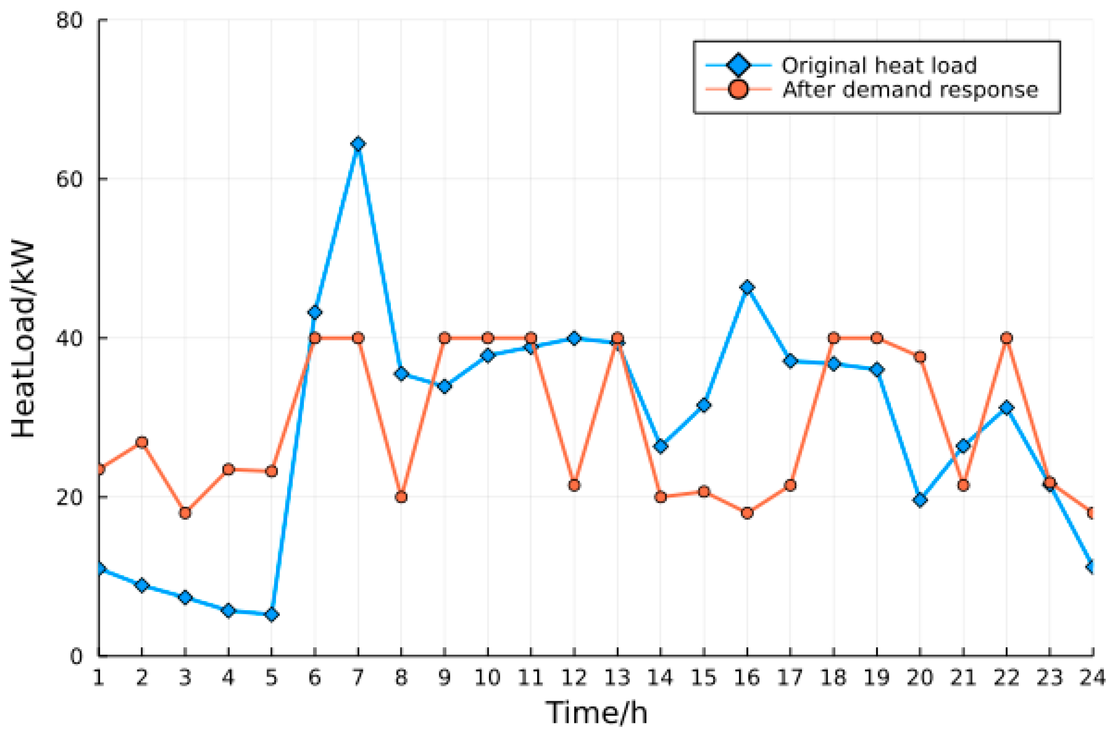
- Heat load model
3. The Solution of the Robust Bilevel Optimization Model
4. Empirical Analysis
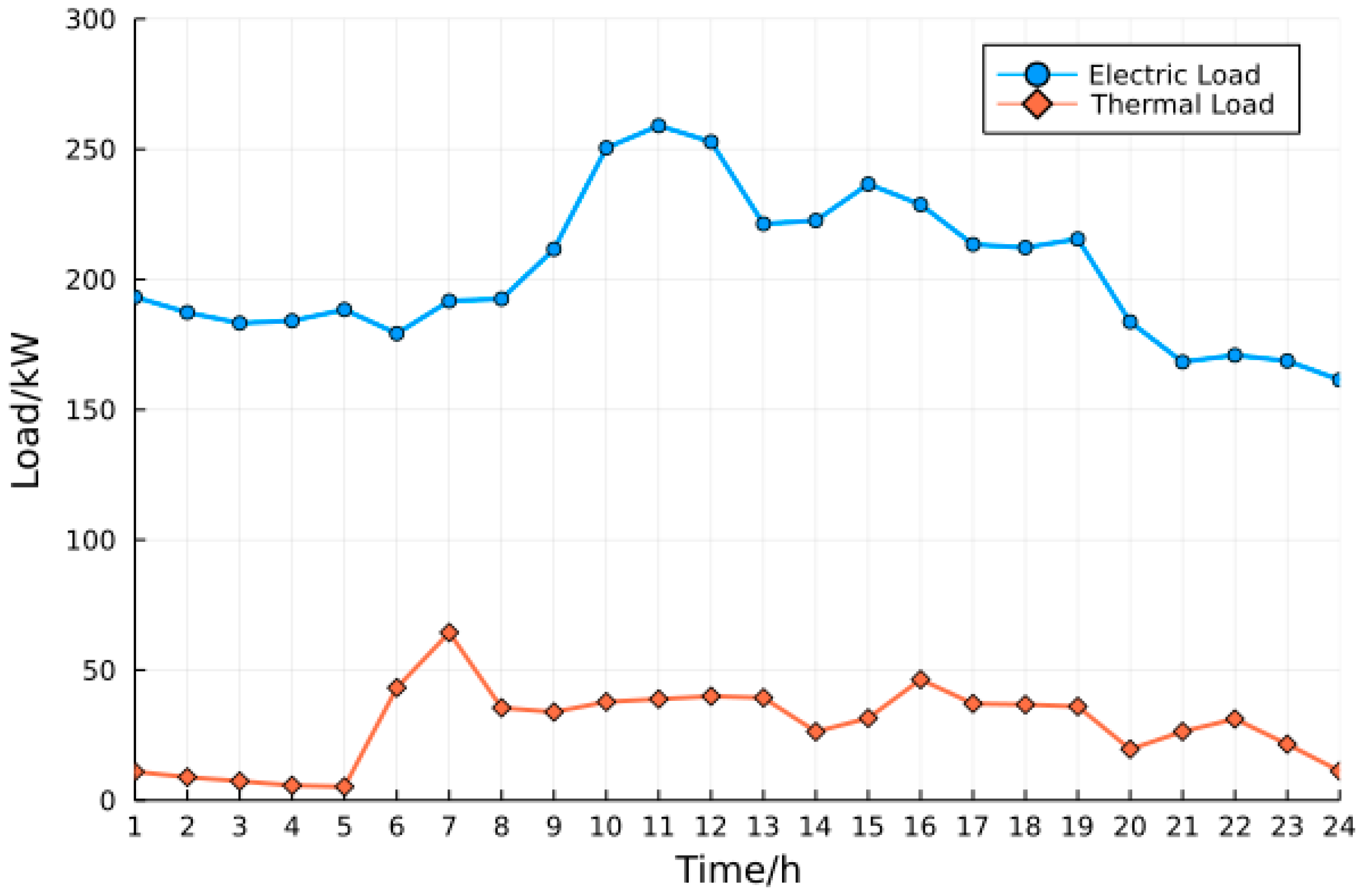
4.1. Description of the Simulation System
4.1.1. PIES Topology
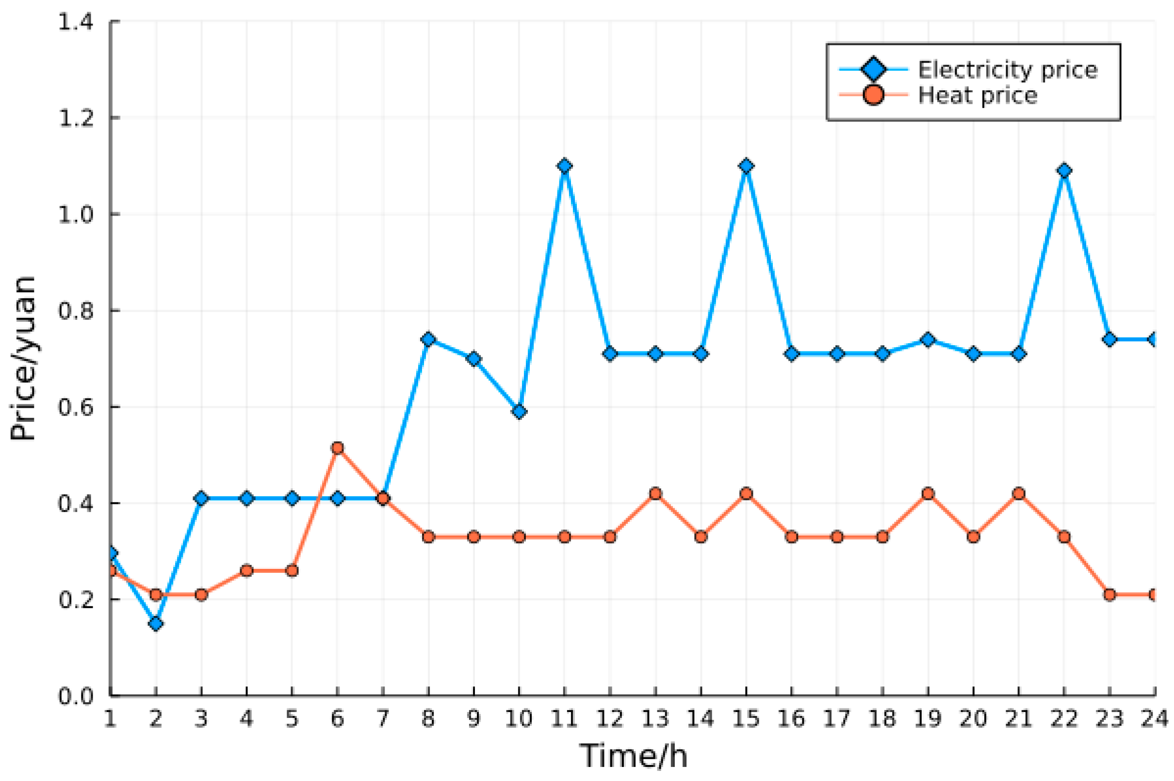
4.1.2. Relevant Data and Model Parameters
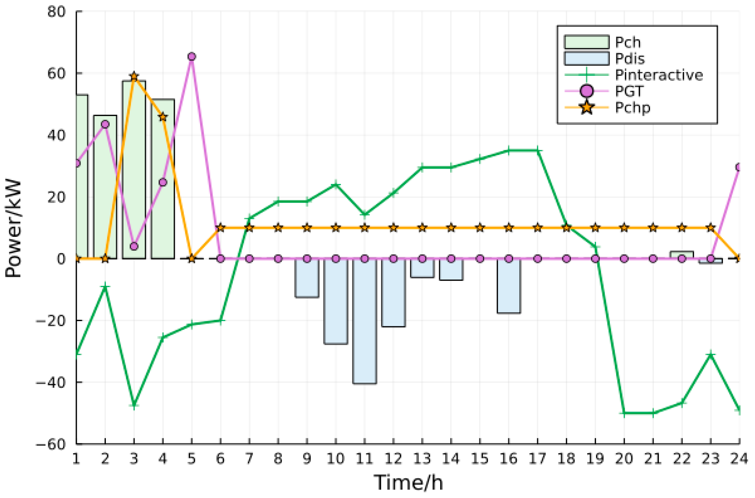
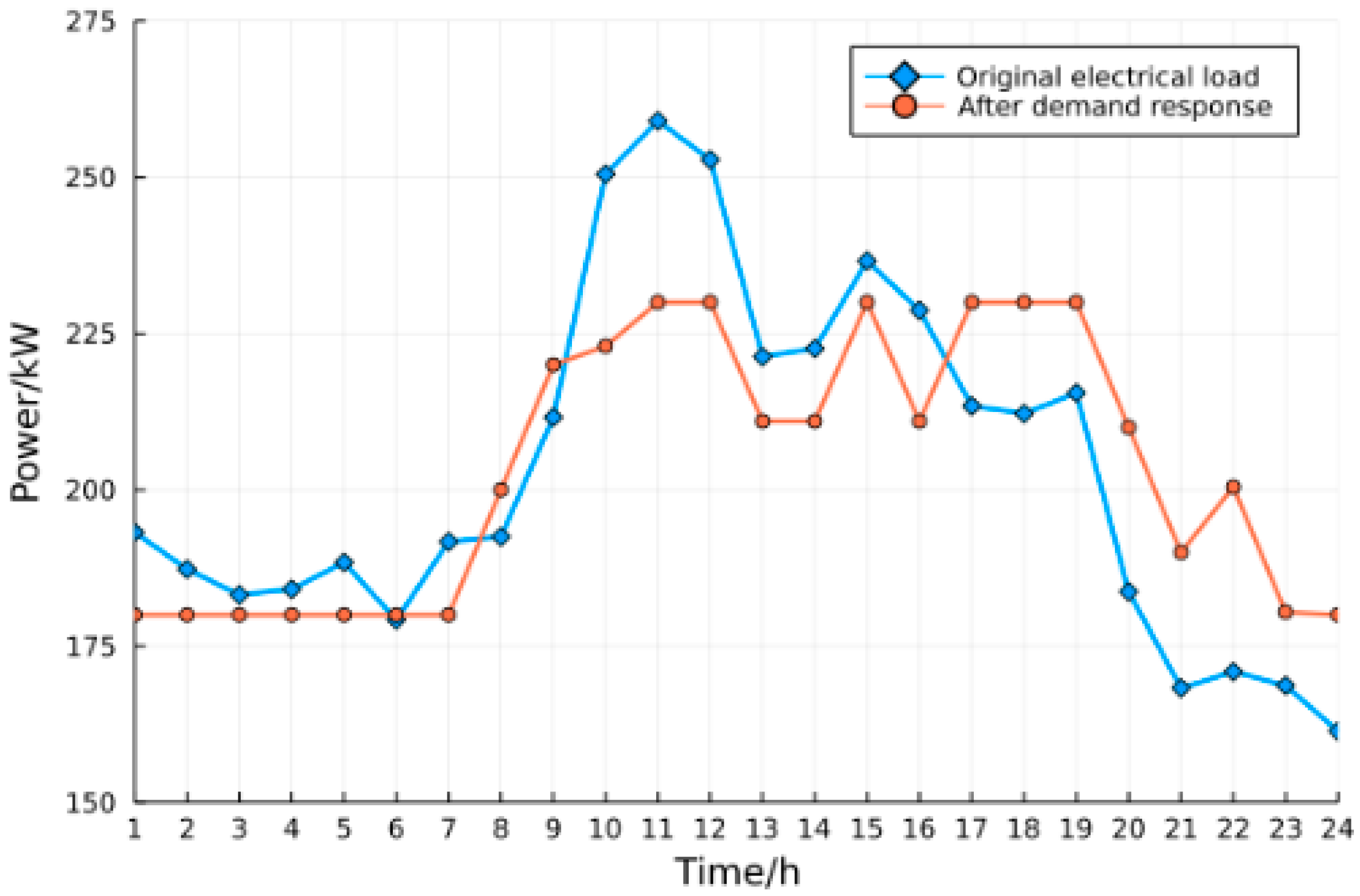
4.2. Simulation Results
4.3. Case Studies
4.3.1. Comparison of Models in Sample
- (1)
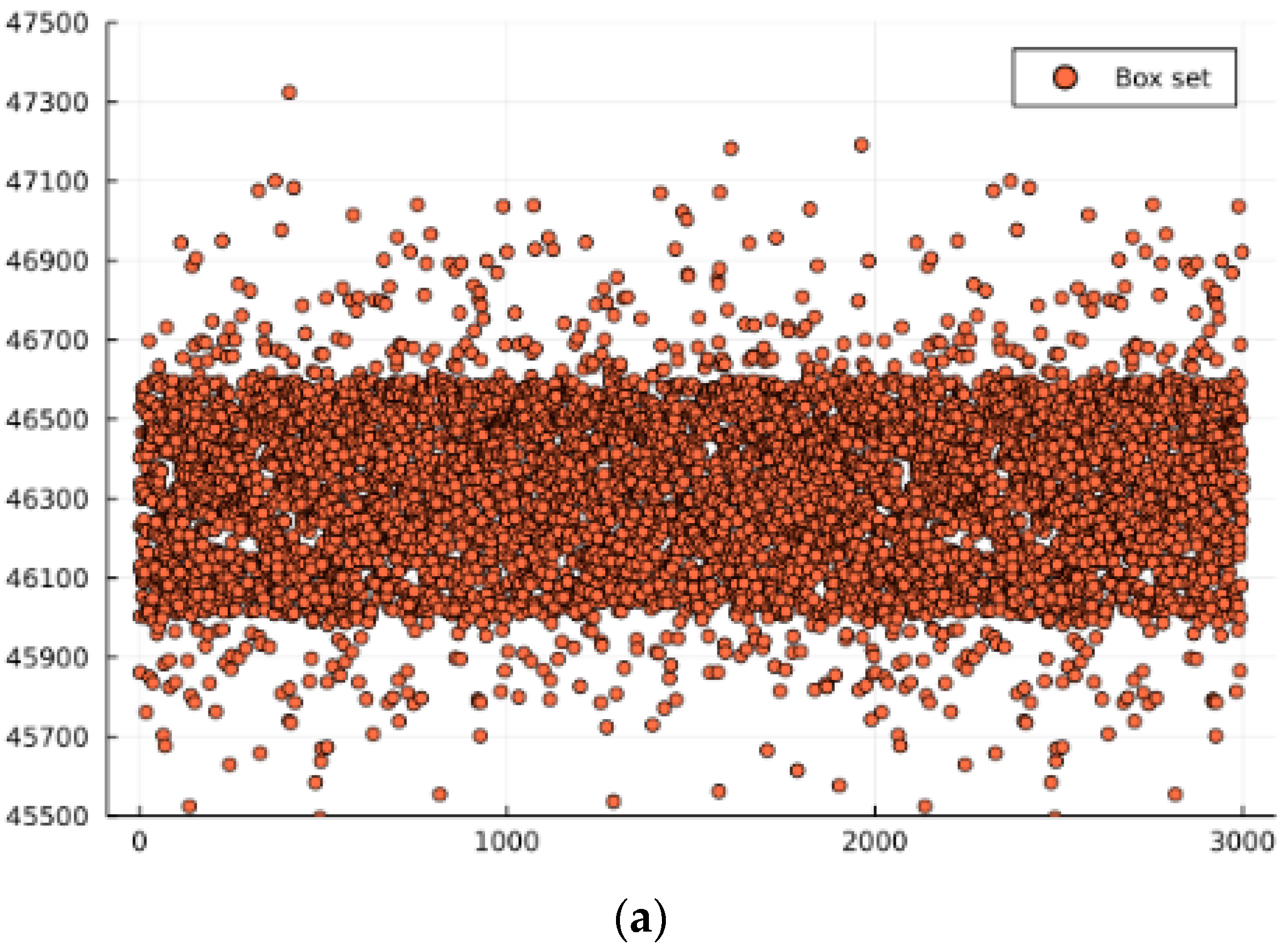
- Box set [44]:
- (2)
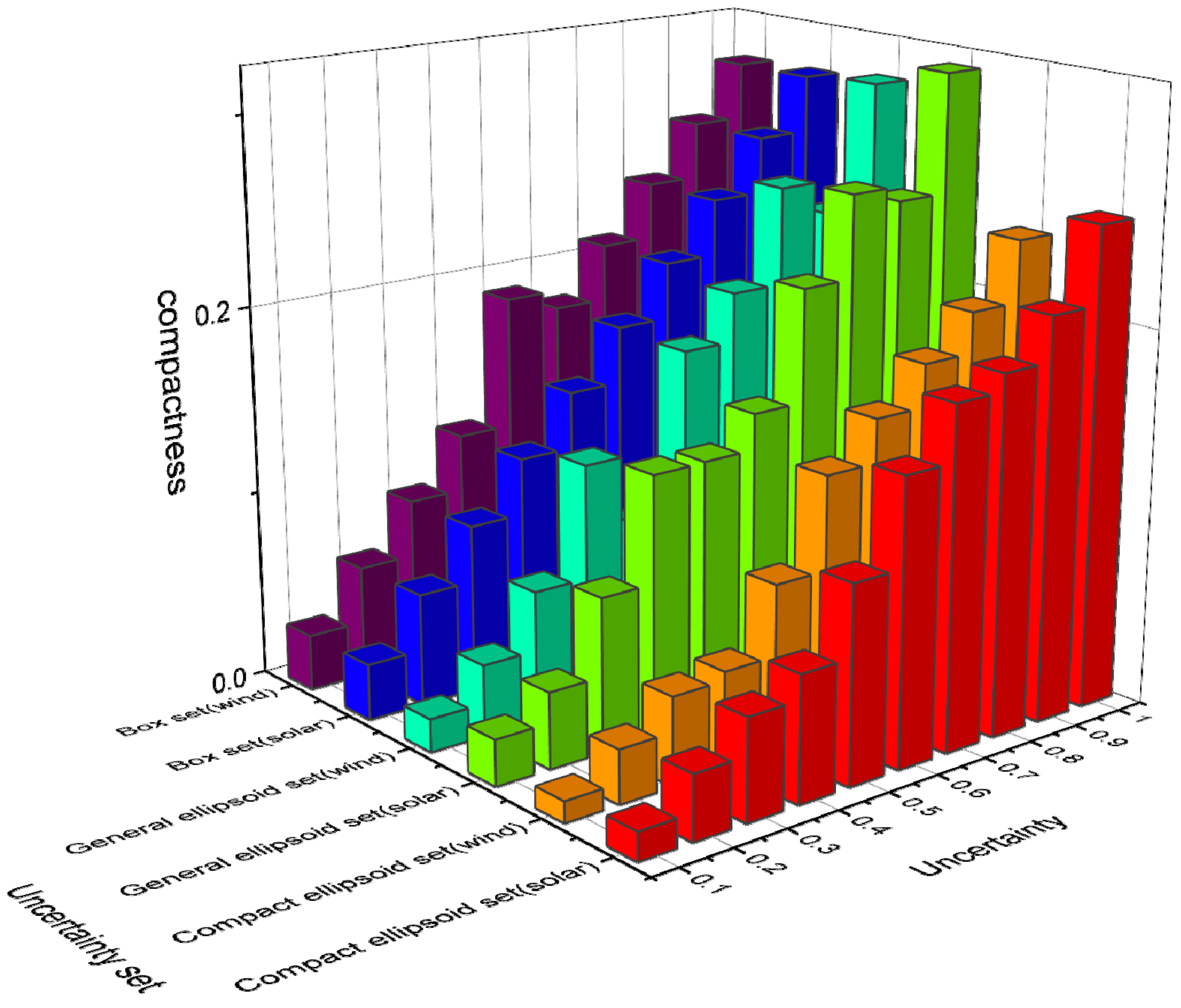
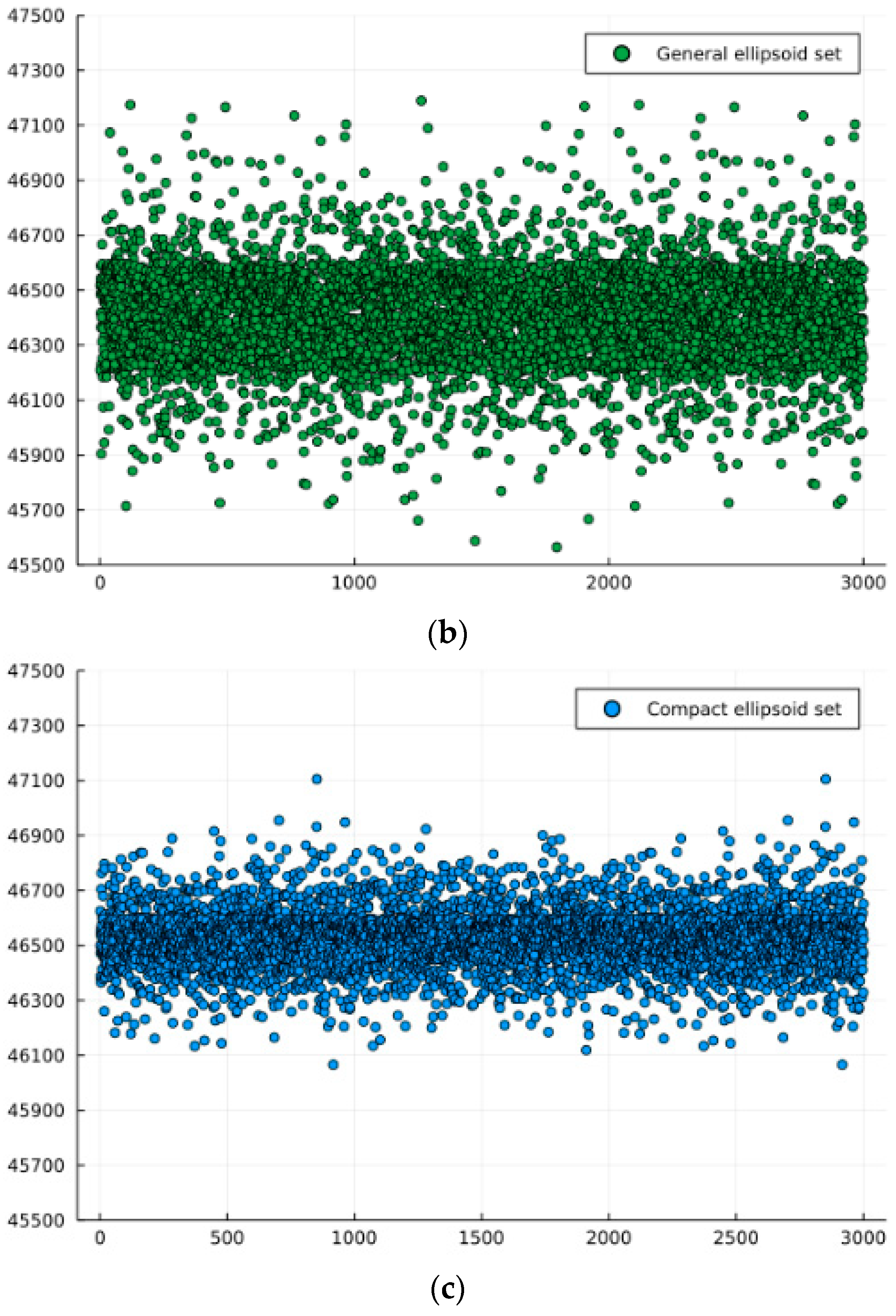
- Ellipsoid Set [45]:
4.3.2. Comparison of Models under Out-of-Sample Simulation
5. Conclusions and Future Work
5.1. Conclusions
5.2. Future Work
Author Contributions
Funding
Data Availability Statement
Conflicts of Interest
References
- Gao, C.; Zhang, Z.; Wang, P. Day-Ahead Scheduling Strategy Optimization of Electric–Thermal Integrated Energy System to Improve the Proportion of New Energy. Energies 2023, 16, 3781. [Google Scholar] [CrossRef]
- Xu, G.; Dong, H.; Xu, Z.; Bhattarai, N. China can reach carbon neutrality before 2050 by improving economic development quality. Energy 2022, 243, 123087. [Google Scholar] [CrossRef]
- Wang, L.; Lin, J.; Dong, H.; Wang, Y.; Zeng, M. Demand response comprehensive incentive mechanism-based multi-time scale optimization scheduling for park integrated energy system. Energy 2023, 270, 126893. [Google Scholar] [CrossRef]
- Xu, Q.; Li, L.; Chen, X.; Huang, Y.; Luan, K.; Yang, B. Optimal economic dispatch of combined cooling, heating and power-Type multimicrogrids considering interaction power among microgrids. IET Smart Grid 2019, 2, 391–398. [Google Scholar] [CrossRef]
- Tan, Z.; Yang, S.; Lin, H.; De, G.; Ju, L.; Zhou, F. Multi-scenario operation optimization model for park integrated energy system based on multi-energy demand response. Sustain. Cities Soc. 2019, 53, 101973. [Google Scholar] [CrossRef]
- Ben-Tal, A.; Ghaoui, L.; Nemirovski, A. Robust Optimization; Princeton University Press: Princeton, NJ, USA, 2009. [Google Scholar]
- Bertsimas, D.; Brown, D.B.; Caramanis, C. Theory and Applications of Robust Optimization. SIAM Rev. 2011, 53, 464–501. [Google Scholar] [CrossRef]
- Chen, F.; Deng, H.; Chen, Y.; Wang, J.; Jiang, C.; Shao, Z. Distributed robust cooperative scheduling of multi-region integrated energy system considering dynamic characteristics of networks. Int. J. Electr. Power Energy Syst. 2023, 145, 108605. [Google Scholar] [CrossRef]
- Kuryatnikova, O.; Ghaddar, B.; Molzahn, D.K. Adjustable Robust Two-Stage Polynomial Optimization with Application to AC Optimal Power Flow. arXiv 2021, arXiv:2104.03107. [Google Scholar]
- Shang, C.; You, F. A data-driven robust optimization approach to scenario-based stochastic model predictive control. J. Process. Control 2019, 75, 24–39. [Google Scholar] [CrossRef]
- Li, F.; Su, J.; Sun, B. An Optimal Scheduling Method for an Integrated Energy System Based on an Improved k-Means Clustering Algorithm. Energies 2023, 16, 3713. [Google Scholar] [CrossRef]
- Massrur, H.R.; Niknam, T.; Fotuhi-Firuzabad, M. Investigation of Carrier Demand Response Uncertainty on Energy Flow of Renewable-Based Integrated Electricity–Gas–Heat Systems. IEEE Trans. Ind. Informatics 2018, 14, 5133–5142. [Google Scholar] [CrossRef]
- Taheri, B.; Jabari, F.; Foroud, A.A. A green cogeneration microgrid composed of water-source heat pumps, a gravity energy storage, and a bio-fueled gas turbine: Design and techno-economic optimization. Sustain. Cities Soc. 2023, 95, 104594. [Google Scholar] [CrossRef]
- Pastore, L.M. Combining Power-to-Heat and Power-to-Vehicle strategies to provide system flexibility in smart urban energy districts. Sustain. Cities Soc. 2023, 94, 104548. [Google Scholar] [CrossRef]
- Lu, Q.; Guo, Q.; Zeng, W. Optimal dispatch of community integrated energy system based on Stackelberg game and integrated demand response under carbon trading mechanism. Appl. Therm. Eng. 2023, 219, 119508. [Google Scholar] [CrossRef]
- Liu, Z.; Li, C. Low-Carbon Economic Optimization of Integrated Energy System Considering Refined Utilization of Hydrogen Energy and Generalized Energy Storage. Energies 2023, 16, 5700. [Google Scholar] [CrossRef]
- Kong, D.; Jing, J.; Gu, T.; Wei, X.; Sa, X.; Yang, Y.; Zhang, Z. Theoretical Analysis of Integrated Community Energy Systems (ICES) Considering Integrated Demand Response (IDR): A Review of the System Modelling and Optimization. Energies 2023, 16, 4129. [Google Scholar] [CrossRef]
- De, G.; Wang, X.; Tian, X.; Xu, T.; Tan, Z. A Collaborative Optimization Model for Integrated Energy System Considering Multi-Load Demand Response. Energies 2022, 15, 2033. [Google Scholar] [CrossRef]
- Zheng, W.; Lu, H.; Zhang, M.; Wu, Q.; Hou, Y.; Zhu, J. Distributed Energy Management of Multi-Entity Integrated Electricity and Heat Systems: A Review of Architectures, Optimization Algorithms, and Prospects. IEEE Trans. Smart Grid 2023. Early Access. [Google Scholar] [CrossRef]
- Singh, M.K.; Kekatos, V. Natural Gas Flow Solvers Using Convex Relaxation. IEEE Trans. Control Netw. Syst. 2020, 7, 1283–1295. [Google Scholar] [CrossRef]
- Ding, J.; Gao, C.; Song, M.; Yan, X.; Chen, T. Optimal operation of multi-agent electricity-heat-hydrogen sharing in integrated energy system based on Nash bargaining. Int. J. Electr. Power Energy Syst. 2023, 148, 108930. [Google Scholar] [CrossRef]
- Yang, S.; Tan, Z.; Zhou, J.; Xue, F.; Gao, H.; Lin, H.; Zhou, F. A two-level game optimal dispatching model for the park integrated energy system considering Stackelberg and cooperative games. Int. J. Electr. Power Energy Syst. 2021, 130, 106959. [Google Scholar] [CrossRef]
- Qin, X.; Sun, H.; Shen, X.; Guo, Y.; Guo, Q.; Xia, T. A generalized quasi-dynamic model for electric-heat coupling integrated energy system with distributed energy resources. Appl. Energy 2019, 251, 113270. [Google Scholar] [CrossRef]
- Wang, S.; Wu, Z.; Zhuang, J. Optimal Dispatching Model of CCHP Type Regional Multi-microgrids Considering Interactive Power Exchange Among Microgrids and Output Coordination Among Micro-sources. Zhongguo Dianji Gongcheng Xuebao/Proc. Chin. Soc. Electr. Eng. 2017, 37, 7185–7194. [Google Scholar]
- Beck, Y.; Ljubić, I.; Schmidt, M. A survey on bilevel optimization under uncertainty. Eur. J. Oper. Res. 2023, 311, 401–426. [Google Scholar] [CrossRef]
- Nasiri, N.; Zeynali, S.; Ravadanegh, S.N. A tactical transactive energy scheduling for the electric vehicle-integrated networked microgrids. Sustain. Cities Soc. 2022, 83, 103943. [Google Scholar] [CrossRef]
- Burtscheidt, J.; Claus, M. Bilevel Linear Optimization Under Uncertainty. In Bilevel Optimization: Advances and Next Challenges; Dempe, S., Zemkoho, A., Eds.; Springer International Publishing: Cham, Switzerland, 2020; pp. 485–511. [Google Scholar]
- Wu, Y.; Yao, L.; Liao, S.; Liu, Y.; Li, J.; Wang, X. A Peak Shaving Method of Aggregating the Distributed Photovoltaics and Energy Storages Based on the Improved K-means++ Algorithm. Dianwang Jishu/Power Syst. Technol. 2022, 46, 3923–3931. [Google Scholar]
- Zhao, S.; Yao, J.; Li, Z. Wind Power Scenario Reduction Based on Improved K-means Clustering and SBR Algorithm. Dianwang Jishu/Power Syst. Technol. 2021, 45, 3947–3954. [Google Scholar]
- Kocuk, B.; Dey, S.S.; Andy Sun, X. Strong SOCP relaxations for the optimal power flow problem. Oper. Res. 2016, 64, 1177–1196. [Google Scholar] [CrossRef]
- Li, P.; Wu, D.; Li, Y.; Liu, H.; Wang, N.; Zhou, X. Optimal Dispatch of Multi-microgrids Integrated Energy System Based on Integrated Demand Response and Stackelberg game. Zhongguo Dianji Gongcheng Xuebao/Proc. Chin. Soc. Electr. Eng. 2021, 41, 1307–1321. [Google Scholar]
- Chai, B.; Chen, J.; Yang, Z.; Zhang, Y. Demand Response Management with Multiple Utility Companies: A Two-Level Game Approach. IEEE Trans. Smart Grid 2014, 5, 722–731. [Google Scholar] [CrossRef]
- Maharjan, S.; Zhu, Q.; Zhang, Y.; Gjessing, S.; Basar, T. Dependable Demand Response Management in the Smart Grid: A Stackelberg Game Approach. IEEE Trans. Smart Grid 2013, 4, 120–132. [Google Scholar] [CrossRef]
- Beck, Y.; Schmidt, M. A Gentle and Incomplete Introduction to Bilevel Optimization; Trier University: Trier, Germany, 2021. [Google Scholar]
- Beck, Y.; Schmidt, M. A Robust Approach for Modeling Limited Observability in Bilevel Optimization. Oper. Res. Lett. 2021, 49, 752–758. [Google Scholar] [CrossRef]
- Beck, Y.; Ljubić, I.; Schmidt, M. A Brief Introduction to Robust Bilevel Optimization. arXiv 2022, arXiv:2211.16072. [Google Scholar]
- Pineda, S.; Morales, J.M. Solving Linear Bilevel Problems Using Big-Ms: Not All That Glitters Is Gold. IEEE Trans. Power Syst. 2019, 34, 2469–2471. [Google Scholar] [CrossRef]
- Fortuny-Amat, J.; McCarl, B. A Representation and Economic Interpretation of a Two-Level Programming Problem. J. Oper. Res. Soc. 1981, 32, 783–792. [Google Scholar] [CrossRef]
- Julia Computing, Inc. JuliaPro Documentation. 2022. Available online: https://juliacomputing.com/docs/ (accessed on 3 October 2023).
- Gurobi Optimizer 9.1. Available online: http://www.gurobi.com (accessed on 3 October 2023).
- Tian, Y.; Liao, Q.; Liu, D.; Zhu, Z.; Peng, S.; Xu, Y. Planning of urban distribution network considering the integrated energy supply-side reform. Power Syst. Technol. 2016, 40, 2924–2933. [Google Scholar]
- Qin, X.; Shen, X.; Guo, Y.; Pan, Z.; Guo, Q.; Sun, H. Combined Electric and Heat System Testbeds for Power Flow Analysis and Economic Dispatch. CSEE J. Power Energy Syst. 2021, 7, 34–44. [Google Scholar] [CrossRef]
- Zhou, X.; Bao, Y.Q.; Ji, T.; Wang, Q. Two-Layer Optimization Scheduling Model of Integrated Electricity and Natural Gas Energy System Considering the Feasibility of Gas-Fired Units’ Reserve. IEEE Access 2020, 8, 40337–40346. [Google Scholar] [CrossRef]
- Jiang, S.-L.; Peng, G.; Bogle, I.D.L.; Zheng, Z. Two-stage robust optimization approach for flexible oxygen distribution under uncertainty in integrated iron and steel plants. Appl. Energy 2022, 306, 118022. [Google Scholar] [CrossRef]
- Sadat, S.A. Optimal Bidding Strategy for a Strategic Power Producer Using Mixed Integer Programming. Ph.D. Thesis, University of South Florida, Tampa, FL, USA, 2017. [Google Scholar]


| Equipment | Parameters | Values |
|---|---|---|
| CHP | Heat-Electricity Ratio | 1.25 |
| Electrical efficiency | 0.25 | |
| Gas tur-bine | Gas calorific value | 39 MJ/m3 |
| Electrical efficiency | 0.55 | |
| Gas boiler | Thermal efficiency | 0.92 |
| Storage device | The upper limit of the capacity | 0.5 MWh |
| The lower limit of the capacity | 0.05 MWh | |
| The upper limit of absorbing energy | 80 kW | |
| The lower limit of absorbing energy | 0 kW | |
| The upper limit of releasing energy | 125 kW | |
| The lower limit of releasing energy | 0 kW |
| Period | Gas Price/Yuan | Interaction Price with Distribution Network/Yuan |
|---|---|---|
| 1:00—7:00 | 3.5 | 0.41 |
| 8:00—10:00, 23:00—24:00 | 5.5 | 0.74 |
| 11:00—22:00 | 6.8 | 1.1 |
| Case | Total Profit/Yuan | Revenue from Electricity Sales/Yuan | Revenue from Thermal Sales/Yuan | Operating Cost/Yuan | Interaction Cost/Yuan |
|---|---|---|---|---|---|
| 1 | 46,978.81 | 32,674.56 | 26,437.56 | 12,142.88 | −9.57 |
| 2 | 44,216.74 | 32,863.86 | 27,653.01 | 16,308.92 | −8.79 |
| 3 | 47,388.26 | 32,674.56 | 26,437.56 | 11,316.00 | −27.17 |
| Case | Line Power/p.u. | ||||
|---|---|---|---|---|---|
| 1–2 | 1–3 | 1–4 | 2–5 | 2–6 | |
| 1 | 0.756 | 0.425 | 0.684 | 0.129 | 0.840 |
| 3 | 1.527 | 0.762 | 1.01 | 0.156 | 1.667 |
| Case | Pipeline Flux/p.u. | ||||
| 1–3 | 2–3 | 3–4 | 6–5 | ||
| 1 | 0.452 | 0.467 | 0.919 | 0.893 | |
| 3 | 0.667 | 0.792 | 1.459 | 1.144 | |
| Uncertainty | Box Set | General Ellipsoid Set | Compact Ellipsoid Set |
|---|---|---|---|
| 97.32% | 96.51% | 98.45% | |
| 98.67% | 97.18% | 99.99% | |
| 99.28% | 96.98% | 100% | |
| 100% | 98.79% | 100% | |
| 100% | 99.02% | 100% | |
| 100% | 100% | 100% | |
| 100% | 100% | 100% | |
| 100% | 100% | 100% | |
| 100% | 100% | 100% | |
| 100% | 100% | 100% |
| Uncertainty Set | Expected Values/Yuan | Root Mean Square/Yuan |
|---|---|---|
| Box set | 46,305.98 | 210.44 |
| General ellipsoid set | 46,401.58 | 187.75 |
| Proposed ellipsoid set | 46,522.61 | 98.24 |
Disclaimer/Publisher’s Note: The statements, opinions and data contained in all publications are solely those of the individual author(s) and contributor(s) and not of MDPI and/or the editor(s). MDPI and/or the editor(s) disclaim responsibility for any injury to people or property resulting from any ideas, methods, instructions or products referred to in the content. |
© 2023 by the authors. Licensee MDPI, Basel, Switzerland. This article is an open access article distributed under the terms and conditions of the Creative Commons Attribution (CC BY) license (https://creativecommons.org/licenses/by/4.0/).
Share and Cite
Wang, P.; Zheng, L.; Diao, T.; Huang, S.; Bai, X. Robust Bilevel Optimal Dispatch of Park Integrated Energy System Considering Renewable Energy Uncertainty. Energies 2023, 16, 7302. https://doi.org/10.3390/en16217302
Wang P, Zheng L, Diao T, Huang S, Bai X. Robust Bilevel Optimal Dispatch of Park Integrated Energy System Considering Renewable Energy Uncertainty. Energies. 2023; 16(21):7302. https://doi.org/10.3390/en16217302
Chicago/Turabian StyleWang, Puming, Liqin Zheng, Tianyi Diao, Shengquan Huang, and Xiaoqing Bai. 2023. "Robust Bilevel Optimal Dispatch of Park Integrated Energy System Considering Renewable Energy Uncertainty" Energies 16, no. 21: 7302. https://doi.org/10.3390/en16217302