Abstract
Installing solar photovoltaic panels on building rooftops can help property managers generate renewable energy and reduce electricity costs. However, the existence of multiple efficiency indicators and ambiguity in interpreting these metrics limits the comparison of the performance of individual installation projects. This paper presents a methodology using data envelopment analysis to evaluate suitable candidates for rooftop solar panel installation. This approach integrates rooftop area, solar irradiation, temperature, costs, energy yield, and revenue to evaluate the relative efficiency of each building. To demonstrate the methodology, it was applied to rank 22 residential buildings, revealing the top performers for installation in 2022. The approach was subsequently adapted to assess potential outcomes under deferred implementation up to 2030, encompassing a diverse range of climate and pricing scenarios. Five installations were found to be optimal irrespective of the future scenarios. In addition, a super-efficiency approach was applied to overcome the low level of discrimination among the possible installations and to rank each individual unit uniquely. The analysis is designed to guide property owners in identifying favorable solar photovoltaic investments within their portfolios under changing conditions.
1. Introduction
In 2018, residential systems accounted for 49% of the market share of installed grid-connected photovoltaic (PV) power in Sweden [1]. This confirms that electricity generation associated with building-integrated projects is an important segment of the solar PV market. Beginning in 2007, grid-connected PV installations consistently surpassed off-grid installations in Sweden. A grid-connected market consists mainly of distributed roof-mounted systems installed by individual homeowners, companies, municipalities, and farmers [2]. The dynamics of energy markets with regard to climate change and economic conditions are almost impossible to predict with certainty [3]. Petrovich et al. [4] addressed the impact of policy and market risks on household investment decisions on residential solar PV systems. It was found that policy uncertainty significantly reduces households’ willingness to invest in solar energy, while market risks, such as fluctuating electricity prices, have less of a deterrent effect. Therefore, the growth in residential solar power installations may slow owing to these uncertainties.
Previous studies [5,6] have discussed the idea that the increase in average global temperature due to global warming might positively affect power generation from PV systems, but the extent of these effects varies from region to region. The projection that rooftop PV systems in most Australian cities will peak in the 2030s and decline by the 2070s was shaped by key factors, including electricity generation, system cost, and PV generation share [5]. Although these results provide useful information regarding the impact of climate change on power generation from PV systems, the literature has yet to address how climate change might influence the considerations surrounding the installation of rooftop solar panels.
In addition to climate change, economic factors also affect the adoption of PV systems. PV system adoption varies across households within a country owing to factors such as available space, household energy demand, generation profile, and the price of electricity. The adoption of rooftop PV panels can be fostered through financial incentives. Financial initiatives mainly comprise subsidies, loans with low interest rates, tax rebates for energy renovation, and grants [7]. Haegermark et al. [8] found that predicting the economic viability of rooftop PV systems is challenging owing to factors such as market conditions, incentive programs, and building-specific parameters. Lang et al. [9] investigated the investment attractiveness of rooftop PV systems in residential buildings. A model-based approach was used to assess the economic performance measured by the internal rate of return (IRR). The analysis was conducted on multiple scales, first for five representative locations, followed by a global assessment. Rooftop PV systems can provide attractive investment returns without subsidies in many regions. Suggestions were made that self-consumption can serve as a catalyst for investment decisions. However, regions with low electricity prices and fossil fuel subsidies encounter significant barriers in shaping attractive markets.
Socio-economic and spatial econometrics also influence investment decisions for rooftop PV deployment. Rausch and Suchanek [10] identified the socio-economic factors influencing the investment decisions of private households in Germany regarding PV systems. Among these, three factors–quality of life, urbanization, and legislation–were considered the main drivers of investments. Dharshing [11] introduced a spatial dimension and identified the relationship between socio-economic status and PV adoption rates. Regionally adjusted return on investment was found to positively impact PV deployment. However, no clear relationship was observed between settlement structure and PV adoption. Narjabadifam et al. [12] developed an automated method to optimize the layout of solar PV panels on building rooftops based on electricity loading. A rooftop recognition methodology was used to extract the information required to optimize the installations. The objective of the optimization was to maximize the power generation and minimize the purchase of electricity from the grid.
Most prior studies on rooftop solar systems have evaluated their performance using various output-to-input ratios. Metrics such as the payback period, levelized cost of electricity (LCOE), net present value (NPV), and return on investment are commonly used to assess the financial viability of residential PV investments [11]. For instance, Ninsawat and Hossain [13] provided an approach for assessing urban rooftop solar potential using geospatial data and modeling individual building characteristics. The payback period varied from 7 to 13 years, depending on the roof type, direction, and shading. Although it is straightforward to compute and interpret these ratios, their use limits the performance comparison among individual installation projects. Their dependence on predefined relationships between inputs and outputs can restrict their flexibility in various scenarios.
Vimpari and Junnila [14] argued that rooftop PVs should be evaluated based on the value they create for the property owner and not the LCOE. Rooftop PVs are already profitable for one-third of the residential building stock and will be profitable for a quarter of the commercial building stock by 2025 in the Helsinki Metropolitan Area. The study demonstrated a substantial increase in the diffusion rate of rooftop PVs through net metering, and the benefits of its adoption outweigh the costs. Financial viability was assessed by calculating the payback period and NPV. While this study presents a useful methodology for estimating overall PV adoption rates, it does not provide a prioritization criterion based on the financial viability of property managers. However, the need for future work to examine the property investment angle is highlighted, particularly to understand the valuation and financial implications of rooftop PVs in real estate portfolios.
This study proposes a data envelopment analysis (DEA)-based methodology to enable property owners to find suitable candidates for rooftop solar panel installations across their building portfolios. Unlike individual metrics, which typically focus on single elements, DEA integrates multiple inputs and outputs. The weighting of inputs and outputs is data-driven rather than based on subjectively assigned weights, which removes bias. This capability results in a single efficiency score for each building, facilitating more direct comparisons. Despite previous research on DEA for electricity generation facility assessment [15,16,17,18], its application to rooftop solar energy is limited. To the best of the authors’ knowledge, only Wang and Sueyoshi [19] focused on the relationship between performance and installation location by applying DEA to a large set of rooftop PV installations in California, which limits the generalization of the results when used in cold climates. This study proposes a rank-based metric to aid property owners in identifying the most attractive candidates for PV deployment, whereas Wang and Sueyoshi [19] assessed the performance of existing operating PV installations.
Several factors can slow the installation of rooftop PV systems. Economic uncertainties, such as high upfront costs and unpredictable returns, coupled with the anticipation of technological advancements, often lead to delayed adoption. Regulatory shifts and changes in incentives also contribute to this unpredictability. Physical constraints, such as unsuitable roof conditions and shading issues, directly impact feasibility, whereas complex ownership structures can further complicate decisions. While the long-term trajectory for rooftop PV economics appears positive, the present situation can deter stakeholders from investing optimally in rooftop systems. Another novelty of the present study is its evaluation of how future climate projections and electricity pricing scenarios, coupled with installation delays, affect the selection of rooftop PV system candidates.
2. Methodology
A set of residential buildings owned by a housing company was selected as candidates for installing rooftop solar panels. For each building, a grid-connected system was designed to calculate the specific annual yield, considering two scenarios: one where panels are installed, and the other where the installation is postponed to 2030. In simulations conducted to anticipate future conditions, adjustments were made to account for several factors influencing electricity generation, including climate conditions and PV panel efficiency. The simulation results were then utilized in a data envelopment analysis to identify the most efficient installation among the buildings under each scenario.
2.1. System Design
The main design issues for a grid-connected PV system are the solar module configuration, solar inverter selection, and cabling of the system [20]. A dynamic simulation program with 3D visualization was used to design and simulate various PV systems [21]. The present study utilized it to model the application of PV on building rooftops. Considering roof accessibility, inter-row spacing between rows of PV arrays, and shading impact analysis, the power production was estimated for each case study.
2.2. Decision Making
Data envelopment analysis is a data-oriented approach for evaluating the performance of a set of peer entities [22]. It is a non-parametric linear programming model that labels a relative efficiency score for each candidate when a transformation from multiple inputs to multiple outputs occurs. These candidates are known as Decision Making Units (DMUs) in DEA nomenclature. For each DMU, a measure was obtained based on the ratio of the weighted sum of outputs to the summation of all weighted inputs. The weights were determined using an optimization algorithm [23]. Relative efficiency determines the efficiency of a DMU in producing a certain level of output based on the amount of input usage when compared to other DMUs within the same set.
Distinct from the commonly used output-to-input efficiency, this method integrates multiple inputs and outputs to construct a relative efficiency measure [19], thereby enabling decision-makers to consider multiple inputs and outputs simultaneously. The accuracy of each setup was evaluated in comparison with an ideal operating unit, which provided a deeper insight than the output-to-input ratio analysis. DEA presents an additional benefit of being effective, even when working with small sample sizes. Typically, a general guideline suggests that the minimum number of DMUs should be at least three times greater than the combined total number of inputs and outputs [24].
The popularity of DEA has increased in recent years and a wide range of algorithms have been introduced. It is almost impossible to implement all the available proposals in the literature. Several algorithms were used in this study to evaluate the installations from various perspectives with the aid of the data envelopment analysis toolbox developed by Álvarez et al. [25].
2.2.1. Input and Output Variables
DEA identifies the efficient frontier of DMUs based on the input and output variables. Evaluations based on the efficiency score are directly influenced by whether the inputs and outputs are selected properly to express the performance of the DMUs. The choice of input and output variables can be made on a physical or theoretical basis. Alternatively, expert knowledge or common practice can be useful in determining these variables. Developing an all-inclusive model that captures all factors associated with the econometrics of rooftop PV electricity generation is impossible. In this study, four inputs and two outputs were introduced to evaluate the system performance.
The following four indicators represent the model inputs.
Insolation: This is a measure of solar energy that is incident on a specified area, which is recorded over a period of time. In the photovoltaic industry, it is commonly expressed as the average irradiance in kilowatt-hours per square meter (kWh/m2) or (kWh/m2/Day) when the time factor is considered. As PV production is strongly dependent on absorbed solar energy, it is a prominent factor in our evaluation.
Roof area: Building codes and permits regulate how PV systems should be mounted on roofs. Rooftop geometry and legislation are two key issues that reduce usable roof area. For example, chimneys, ventilation pipes, and dormers are typical obstructions on roofs. In addition, there are roof areas shaded by trees or neighboring buildings that restrict the use of all available roof areas. In this study, a solar panel layout utilizing the maximum number of modules, preferably towards the south, for the available roof area was designed. It is worth mentioning that for all buildings, a monocrystalline PV module was selected. The specifications of the PV modules are listed in Table 1.

Table 1.
PV module specifications [26].
Costs: This variable entails expenses associated with the initial investments for the modules, inverters, and cabling, plus operational and maintenance costs, which are dependent on factors such as system size, optional components, and difficulty level of installations. Generally, PV systems have low operational and maintenance costs. The costs were calculated according to the CRAVEzero project report guideline [27].
Ambient temperature: The efficiency of PV electricity generation is inevitably affected by the variability in weather conditions. In this study, hourly values of ambient air temperature were derived from the Meteonorm software database for the current climate scenario as well as future projections [28]. An increase in temperature results in a reduction in photovoltaic power output. This method treats ambient air temperature as an undesirable indicator; hence, its inverse was considered a factor in the DEA, similar to [19].
The following two variables were used as outputs.
Specific annual yield: The specific annual yield is defined as the total alternating current (AC) energy output from the inverter generated by the power system during a year divided by the rated PV array power.
Annual income: Grid-tied solar systems export all generated electricity to the grid and eliminate the need for battery storage if they operate in a full-feed-in condition. The electricity rate structures and financial revenues of electricity sold to the grid are highly correlated. This dependency becomes more challenging, as customers are allowed to choose their electricity company and negotiate the best possible deal. Here, it is assumed that all generated electricity is purchased by Nord Pool AS, a leading power market in Europe. The selling price of electricity consists of various components, such as spot market price, electricity certificates, grid compensation, and tax deduction [29]. When production is sold to the grid at a minimum, it is valued at the market hourly spot price plus a 0.05 for grid compensation [30]. Additional revenue from production can arise from green certificates valued at 0.1 . Since 2015, microproducers of renewable electricity have been eligible for tax deductions for feed-in electricity. The tax deduction amounts to 0.6 of the renewable electricity fed into the grid during a calendar year. There is currently no end date for tax deductions, but it is highly probable that they will be removed in the near future [31]. Therefore, tax deductions were omitted from the current analysis. For each installation, the total amount of energy fed to the grid was calculated monthly over the course of the year. This monthly energy calculation was then multiplied by the corresponding electricity selling price for that month to represent annual income.
2.2.2. Modeling
The most widely used DEA formulations are the standard CCR model presented by Charnes et al. [32] and the BCC model presented by Banker et al. [33]. DEA models can be classified according to their orientation. The input-oriented model searches for optimal input values corresponding to a desirable level of output, and the output-oriented model maximizes the output while the input is kept at a constant level. The orientation of the model should be selected according to whether the decision-maker has the most control over the inputs or outputs. It makes sense to use an output-oriented model because the main target is output enhancement rather than input reduction.
The foremost performance measure was introduced by Charnes, Cooper and Rhodes [32]. Assume DMUs with inputs and outputs exist. So, the number of DMUs are the same as the number of buildings. The values of inputs and outputs of are represented by and , respectively. The efficiency of , relative to other DMUs in an output-oriented CCR multiplier format is calculated, as follows [32]:
where weights of inputs and outputs for are denoted by and , respectively. Constraints are set to confirm that all efficiencies are below one, and the input and output weights are all positive. Suppose that the optimal solutions of the CCR model are denoted by and . Consequently, the efficiency for is calculated by . This optimization problem should be solved times (for each DMU) to obtain sets of input and output weights.
The CCR model is interpreted as constant returns to scale, meaning that a proportionate increase in inputs results in an increase in output by the same proportion. This assumption implies that the DMU’s scale of operation does not affect its efficiency. To accommodate scenarios with variable returns to scale, an alternative DEA model was introduced by Banker, Charnes and Cooper [33]. The BCC model allows an increase in the input values, resulting in a nonproportional increase in output levels. An output-oriented BCC model written in the multiplier format is formulated as follows:
where weights of inputs and outputs for are denoted by and , respectively. Constraints are set to confirm that all efficiencies are below one and the input and output weights are all positive. Suppose that the optimal solutions of the BCC model are denoted by and . Consequently, the efficiency for is calculated by . This optimization problem should be solved times (for each DMU) to obtain sets of input and output weights.
If a DMU is fully efficient in both CCR and BCC scores, it operates at the most productive scale size. If a DMU has full BCC efficiency but a low CCR score, it operates locally efficiently but not globally efficiently because of the scale size of the DMU [34]. Thus, it is reasonable to characterize the scale efficiency of a DMU based on the ratio of the two scores. The scale efficiency score for each unit was calculated by dividing the CCR efficiency by the BCC efficiency [34]:
Scale efficiency provides a basis for benchmarking and comparing installations operating at different scales. This enables fair comparisons by considering the inherent scale differences among case studies. By considering scale efficiency, the relative performance of solar-powered buildings can be evaluated, even if their sizes or production levels differ significantly. The scale efficiency score indicates whether rooftop panels are installed at the most productive size. If the scale efficiency score is less than one, then the DMU either wastes resources (e.g., cost and area) or is less productive relative to its optimal size.
The above-mentioned models serve the purpose of identifying efficient and inefficient DMUs, but they do not provide a direct ranking among efficient DMUs. Additional methods have been developed to rank efficient DMUs. Among these methods, Andersen and Petersen [35] proposed an extension of traditional DEA models that permits a unique ranking for efficient DMUs. In traditional DEA models, efficient DMUs all have an efficiency score of 100%, as they lie on the efficiency frontier. The super-efficiency model allows the ranking of these efficient DMUs. Assume DMUs with inputs and outputs exist. So, the number of DMUs are the same as the number of buildings. The values of inputs and outputs of are represented by and , respectively. The scores for inefficient DMUs remain the same as those in the standard models. However, the super-efficiency of is obtained by solving the following linear programming model [36]:
where the is excluded from the reference set. is the weighting variable assigned to each in the reference set.
2.3. Projection Scenarios
Future climate scenarios are generated at various scales to explore how anthropogenic activities might interact with Earth’s biogeochemical cycles, thereby affecting its climate system. Projections can be distinguished by the sophistication level of each climate model [37]. From the variable sets of this project, the ambient air temperature and solar radiation are the two key parameters that are influenced by climate change. The Meteonorm weather generator tool [38] was used to create the future weather datasets. By integrating the climate database with the spatial interpolation of the principal weather variables and a stochastic weather generator, the tool generates hourly weather data for any site in the world. Weather variables, such as global irradiance on a horizontal plane at ground level and dry-bulb temperature, were provided by the tool. This tool can also be used in climate change studies. Representative Concentration Pathways (RCPs) under the Intergovernmental Panel on Climate Change (IPCC) Fourth Assessment Report (AR4) [39] were used in the tool to generate future weather data for different emission scenarios for 2030. RCPs are a set of pathways developed by the climate modeling community as a basis for long-term and near-term modeling experiments. These pathways predict how the concentration of greenhouse gases in the atmosphere will change in the future because of human activity. Weather files were generated based on the three RCPs selected in the current study. These three RCPs range from very high (RCP8.5) to low (RCP2.6) future concentrations, and an intermediate scenario (RCP4.5) in between. The lower the RCP number, the more aggressive the mitigation measures taken, including deploying renewable energy and improving efficiency. RCP2.6 represents a best-case sustainability scenario for 2030, while RCP8.5 assumes continued high emission growth. A detailed discussion of these models can be found in [40].
According to the CRAVEzero project report guidelines [27], solar PV panels have notable potential for cost reduction. The projection utilized learning curve theory, which assumes that costs decline as cumulative production volumes increase. To capture the full scope of PV costs, the report considered multiple categories beyond hardware. These include module production costs, which are expected to decrease through manufacturing optimization and efficiency gains. The balance of system costs, such as wiring, mounting structures, and installation labor, were also factored in. Additional soft costs related to permitting, marketing, and administration were also incorporated. The overhead and financing costs linked to PV projects were also included in the holistic evaluation. As observed in Figure 1, installing PV panels in 2030 will cost approximately 13% less than the current price in the European Union.
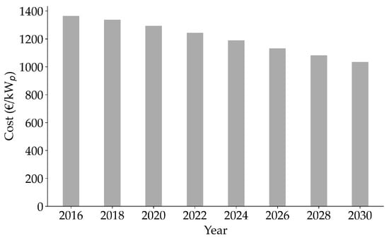
Figure 1.
Cost development of PV based on the CRAVEzero database. Reproduced with permission from [27], Fraunhofer ISE, 2018.
Ott et al. [41] estimated that the module efficiency will exceed 30% after 2030. Goldschmidt et al. [42] also projected that PV module efficiency could fall within the range of 24.1%–25.9% by 2030, considering various scenarios. In this study, the photovoltaic module efficiency in 2030 was assumed to be 25%. Solar PV earnings are a critical indicator for a property holder. In this study, five policy scenarios for electricity spot price development are considered, as presented in Table 2. Scenarios A and E were based on the long-term electricity spot price predictions presented by Rydén et al. [43]. The other three scenarios are based on forecasts generated by the TBATS time-series model, designed to capture key time-series components, such as trend, seasonality, and autoregressive behavior [44]. The forecast was derived from 11 years of monthly historical spot prices covering contracts with deliveries from 2012 to 2022, obtained from the Nord Pool market. TBATS provides uncertainty intervals for forecasts, enabling the evaluation of the potential range of future values, which makes it suitable for long-term forecasts [45]. Scenarios B, C, and D represent the point forecast, confidence ceiling, and confidence floor, respectively. The point forecast represents the most probable future value of the time series. The confidence ceiling, which corresponds to a 90% confidence level, represents the upper boundary of the range within which the actual future value is likely to fall. The confidence floor, corresponding to the 90% confidence level, represents the lower boundary of the range within which the actual future value is likely to fall.
Table 2.
Policy scenarios for electricity spot price development.
Figure 2 shows the price development for each policy action. In the Nord Pool electricity market, Sweden is divided into four bidding areas for trading and pricing electricity. All buildings examined in this study were situated within the SE3 or SE4 bidding areas of Sweden’s electricity market. However, for clarity, only price developments are shown, based on the SE3 historical spot price. An abrupt increase in Sweden’s electricity spot prices began in late 2020. In Scenario B, there is a balanced approach between history and recency, allowing for adaptive responsiveness to recent years while retaining the essential insights gained from past observations. Scenario C indicates that prediction intervals widen more rapidly at longer forecast horizons, as there is less confidence in sustaining historical patterns. Thus, the confidence ceiling shows a greater extrapolation of price volatility from 2020 to 2022. Recent volatility is more likely to affect the upper bound because temporary shocks are unlikely to permanently alter the expected confidence floor values. This could be observed in Scenario D in which the price could fall to the lowest levels since 2012.
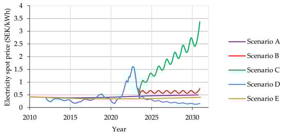
Figure 2.
Potential future electricity prices under various policy scenarios.
The forecasted weather files and module efficiency projections for 2030 were used to simulate the specific annual yield for each scenario.
2.4. Case Study
A detailed study of building typology in Sweden by the National Board of Housing, Building, and Planning divided the building stock into three climatic zones [46]. Solar panel adoption is highest in the southernmost climate zone, which is well-suited for PV applications because of its warmer climate and higher solar insolation. The specific annual yield and annual income were calculated for a dataset consisting of 22 multi-family apartment buildings in climate zone 3. Gothenburg, Västerås, and Stockholm each had six buildings, while the remaining buildings were in Malmö. A statistical description of the input and output variables is provided in Table 3.
Table 3.
Key statistical metrics for rooftop PV system design in 2022.
2.5. Limitations
Data envelopment analysis is a valuable decision-making tool that eases the process of choosing among alternatives. Nevertheless, it is best to examine their inherent properties and pitfalls. DEA is a fully non-parametric estimation method. It is capable of estimating efficiency when multiple inputs are used to produce multiple outputs without the need to specify distributions or functional forms. DEA is notably sensitive to outliers and noise in the dataset. These can not only distort efficiency scores but also affect the overall interpretation of the results. In addition, an efficient frontier is constructed in relation to members within the dataset, and adding new DMUs will change scores or rankings.
The data envelopment analysis results depend on the specific inputs and outputs chosen for the model. There are no definitive guidelines for selecting the DEA variables. The choice often relies on expert judgement, literature review, or trial-and-error testing. The choice of variables impacts the efficiency scores.
It should also be noted that solar irradiation and ambient temperature are time-dependent variables. Average yearly values were used for both indicators. Using average values might not lead to inaccurate results in this study because all buildings are located within the same climate zone in Sweden. If seasonality is critical for any variable in a DEA analysis, one idea is to divide the data into multiple periods and aggregate the scores to form an annual performance measure.
3. Results
The DEA models, which integrate the introduced input and output variables, were initially solved for 2022. Subsequently, an evaluation was conducted to assess the impact of climate change and electricity price development scenarios on efficiency, considering a postponed installation until 2030. The final part of the results section is devoted to the super-efficiency concept, which facilitates decision making among efficient DMUs. Table 4 presents the number of efficient units in each city, as well as the statistical measures for the set in 2022. Across the cities, installations in Västerås emerged as the top performers, with four out of six buildings found to be scale-efficient. In contrast, only one out of six buildings in Malmö operates optimally based on scale efficiency. Overall, nine of the 22 buildings represent the best candidates from an efficiency standpoint for solar panel deployment. An efficiency study is not only limited to the provision of an efficiency score for a unit but also indicates whether there is any room for inefficient units to improve. The results showed that the installations had an average scale efficiency of 0.96, indicating that they operate close to an optimal scale on average. The lowest scale efficiency score was 0.83, indicating that the system operated at an inefficient scale. This implies that the observed installations could have further increased their output by 17% if they had adopted an optimal scale. This may be achieved using a more efficient solar panel or a policy that leads to higher earnings by selling electricity. Another interpretation is that the system can theoretically reduce its inputs by 17% and still produce the current level of outputs. This can be achieved by revising the panel layout and design based on the available roof area. An installer can choose whether to dismiss the installation or check the possibility of achieving higher performance.
Table 4.
Scale efficiency statistics for 2022.
The PV adoption process is moving forward at a slow speed, particularly for residential buildings, owing to grid infrastructure and unrewarded investment risk. Therefore, it may take years to achieve rapid rooftop solar growth. It is of interest to explore the extent of change in decision making if the same panel configurations are installed around 2030. Figure 3 shows how scale efficiency is distributed by postponing project delivery or installation across various climate change scenarios. Each subplot presents the variations in scale efficiency under different electricity spot price projections. For each climate pathway assumption, scale efficiency was evaluated for 2022, as well as other electricity spot price projections for 2030. The analysis pairs each climate pathway with a theoretically feasible future price projection scenario. The boxplot shows several aspects of the scale efficiency distribution. The whiskers extending from the boxes indicate the minimum values of scale efficiency, excluding potential outliers. The lower and upper edges of the blue box mark the first and third quartiles, respectively, whereas the red line inside the box represents the median. The plus signs are potential outliers, with values more than 1.5 times the interquartile range below the first quartile. The horizontal axis tick labels such as ‘2030B’ refer to the calculation based on the electricity price development defined in scenario B for 2030. It is noteworthy that the efficiency distribution shows limited influence from both the climate modeling pathway and electricity projection scenarios. The median scale efficiency based on RCP2.6 for the year 2022 following the climate model is 0.97, while it roughly increases to 0.99, based on spot price projection scenarios B, D, and E. Similar observations can be made for the rest of the scenarios.
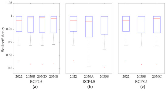
Figure 3.
Statistical distribution of scale efficiency among DMUs for 2022 and 2030 under different future climate scenarios and electricity spot price projections: (a) RCP2.6, (b) RCP4.5, and (c) RCP8.5.
The efficiency scores are relative measures that collectively consider the entire set of DMUs and their performance. In other words, even if the annual income and specific annual yield of individual buildings change in response to different scenarios, the efficiency scores are influenced more by the relative relationships between DMUs rather than their absolute performance changes. If the order of DMUs by efficiency remains relatively stable across scenarios, the overall efficiency scores may not vary significantly. This observation is further supported by the rankings presented in Table 5, in which each DMU’s ranking is closely aligned across diverse scenarios. The number of efficient DMUs in 2022 is nine, which remains the same under the RCP2.6 scenario D in 2030. The low revenue of scenario D caused more Malmö installations to become efficient, even though the number of efficient DMUs remained constant between periods. For scenario A under RCP4.5, scenario C under RCP8.5, and scenario E under RCP2.6, the number of best candidates for rooftop panel installations was 10. It is also revealed that if forecasted price follows scenario B, the number of DMUs operating at an optimal scale increase from 9 in 2022 to 11 in 2030.
Table 5.
Installation ranking comparisons across spot price electricity scenarios and climate projections.
It has been reported that DMU1, DMU3, and DMU12 in Gothenburg, DMU5 in Stockholm, DMU20 and DMU22 in Västerås, and DMU8 in Malmö stand out as prime candidates for initiating a solar installation project, regardless of the upcoming scenario in 2030. For all other scenarios, rank shuffling occurs among DMUs that are not at the efficient frontier. For example, under the RCP2.6 pathway, if the electricity price follows the pattern of scenario D, DMU7 operates at an optimal scale. However, if the price pattern follows scenario E, DMU7 is ranked 11th among its peers. This demonstrates how different price projection scenarios impact property owners’ decisions on selecting the best building candidates for rooftop panel installation in 2030.
One of the main shortcomings of standard DEA models is that all efficient DMUs are ranked equally in terms of their performance. The super-efficiency score allows discrimination across DMUs by calculating an individual score that differs across observations. Table 6 presents the DMU rankings evaluated using the super-efficiency model. DMU5 in Stockholm claims the top rank among all scenarios, whereas DMU16 in Stockholm emerges as the least favorable candidate for solar panel deployment. For most DMUs, the rankings remained relatively stable from 2022 to 2030 across different policy scenarios. The exceptions were DMU10, DMU11, DMU19, and DMU7, which experienced considerable shifts in their rankings.
Table 6.
Installation ranking comparisons for different spot price electricity scenarios based on the super-efficiency model.
4. Discussion
Uncertainty about the economic feasibility of rooftop solar panels and the lack of government policy incentives have hindered their widespread use. To encourage adoption, this study proposes a rank-based method to identify the most suitable buildings for rooftop solar panel installation using data envelopment analysis. This approach allows real estate companies to determine prime solar panel candidates from their portfolios, enabling phased implementation installation on optimal buildings before expansion. The analysis revealed that 9 out of the 22 buildings represented the best candidates from an efficiency standpoint for solar panel deployment.
It is important to acknowledge that real estate companies may face certain limitations that push back the project timeline to execute the installation a few years forward. The method was then applied to gauge the impact of delayed deployment on rankings, considering scenarios for climate change and electricity price projections. Seven buildings (DMU1, DMU3, DMU5, DMU8, DMU12, DMU20, and DMU22) emerged as optimal installation locations, irrespective of the different future scenarios. The super-efficiency approach further discriminated top performers into a ranked order, providing clearer guidance on how to prioritize installation candidates. While this analysis focused on a case study in Sweden, the strategy can be applied to identify favorable solar PV investments across diverse regions and build portfolios. Further research could incorporate additional parameters to extend DEA modeling.
Author Contributions
Conceptualization, N.M., A.V. and E.J.; methodology, N.M. and A.V.; software, N.M.; validation, N.M. and A.V.; formal analysis, N.M.; investigation, N.M.; resources, A.V. and K.K.; data curation, N.M.; writing—original draft preparation, N.M.; writing—review and editing, A.V. and K.K.; visualization, N.M.; supervision, A.V. and K.K.; project administration, A.V. and K.K.; funding acquisition, A.V. All authors have read and agreed to the published version of the manuscript.
Funding
This research was funded by KK-stiftelsen as part of the SMART—Smart control of district heating networks integrating next generation energy-efficient buildings (project No. 14927). The authors would also like to thank Bostads AB Mimer as a project partner and co-financer in the SMART project for providing the measurement datasets. The publishing fees for this article were financed by the Mälardalen University library.
Data Availability Statement
Restrictions apply to the availability of these data. Data were obtained from the Bostads AB Mimer and are available upon request with permission from the Bostads AB Mimer.
Acknowledgments
The authors extend their sincere appreciation to the project developers affiliated with the NEEDs—innovative approaches for energy efficiency improvement for positive or self-balanced districts (project No. 52686-1). By sharing their domain-specific experience and insights, they have indirectly contributed to shaping this paper and its findings.
Conflicts of Interest
The authors declare no conflict of interest. The funders had no role in the design of the study; in the collection, analyses, or interpretation of data; in the writing of the manuscript; or in the decision to publish the results.
Nomenclature
| Symbol | Description |
| n | Number of decision-making units |
| m | Number of inputs |
| s | Number of outputs |
| Input values for the jth decision making unit | |
| Output values for the jth decision making unit | |
| o | Index for an arbitrary decision-making unit |
| Weights for inputs | |
| Weights for outputs | |
| Weighting variable for jth decision making unit | |
| Efficiency | |
| Abbreviations | |
| AC | Alternative current |
| AR4 | Fourth working group |
| BCC | Banker, Charnes, and Cooper |
| CCR | Charnes, Cooper, and Rhodes |
| DEA | Data envelopment analysis |
| DMU | Decision making unit |
| IPCC | Intergovernmental Panel on Climate Change |
| IRR | Internal rate of return |
| LCOE | Levelized cost of electricity |
| NPV | Net present value |
| PV | Photovoltaic |
| RCP | Representative Concentration Pathway |
| SE1, SE2, SE3, SE4 | Electricity regions in Sweden |
| SEK | Swedish krona |
| TBATS | Trigonometric seasonality, Box-Cox transformation, ARMA errors, Trend and Seasonal components. |
References
- Stridh, B.; Yard, S.; Larsson, D.; Karlsson, B. Profitability of PV electricity in Sweden. In Proceedings of the 2014 IEEE 40th Photovoltaic Specialist Conference (PVSC), Denver, CO, USA, 8–13 June 2014; pp. 1492–1497. [Google Scholar]
- Bankel, A.; Mignon, I. Solar business models from a firm perspective—An empirical study of the Swedish market. Energy Policy 2022, 166, 113013. [Google Scholar] [CrossRef]
- Lund, H.; Sorknæs, P.; Mathiesen, B.V.; Hansen, K. Beyond sensitivity analysis: A methodology to handle fuel and electricity prices when designing energy scenarios. Energy Res. Soc. Sci. 2018, 39, 108–116. [Google Scholar] [CrossRef]
- Petrovich, B.; Carattini, S.; Wüstenhagen, R. The price of risk in residential solar investments. Ecol. Econ. 2021, 180, 106856. [Google Scholar] [CrossRef]
- Ma, W.W.; Rasul, M.G.; Liu, G.; Li, M.; Tan, X.H. Climate change impacts on techno-economic performance of roof PV solar system in Australia. Renew. Energy 2016, 88, 430–438. [Google Scholar] [CrossRef]
- Solaun, K.; Cerda, E. Climate change impacts on renewable energy generation. A review of quantitative projections. Renew. Sustain. Energy Rev. 2019, 116, 109415. [Google Scholar] [CrossRef]
- Bertoldi, P.; Economidou, M.; Palermo, V.; Boza-Kiss, B.; Todeschi, V. How to finance energy renovation of residential buildings: Review of current and emerging financing instruments in the EU. WIREs Energy Environ. 2021, 10, e384. [Google Scholar] [CrossRef]
- Haegermark, M.; Kovacs, P.; Dalenback, J.O. Economic feasibility of solar photovoltaic rooftop systems in a complex setting: A Swedish case study. Energy 2017, 127, 18–29. [Google Scholar] [CrossRef]
- Lang, T.; Gloerfeld, E.; Girod, B. Don׳t just follow the sun—A global assessment of economic performance for residential building photovoltaics. Renew. Sustain. Energy Rev. 2015, 42, 932–951. [Google Scholar] [CrossRef]
- Rausch, P.; Suchanek, M. Socioeconomic Factors Influencing the Prosumer’s Investment Decision on Solar Power. Energies 2021, 14, 7154. [Google Scholar] [CrossRef]
- Dharshing, S. Household dynamics of technology adoption: A spatial econometric analysis of residential solar photovoltaic (PV) systems in Germany. Energy Res. Soc. Sci. 2017, 23, 113–124. [Google Scholar] [CrossRef]
- Narjabadifam, N.; Al-Saffar, M.; Zhang, Y.; Nofech, J.; Cen, A.C.; Awad, H.; Versteege, M.; Gül, M. Framework for Mapping and Optimizing the Solar Rooftop Potential of Buildings in Urban Systems. Energies 2022, 15, 1738. [Google Scholar] [CrossRef]
- Ninsawat, S.; Hossain, M.D. Identifying Potential Area and Financial Prospects of Rooftop Solar Photovoltaics (PV). Sustainability 2016, 8, 1068. [Google Scholar] [CrossRef]
- Vimpari, J.; Junnila, S. Estimating the diffusion of rooftop PVs: A real estate economics perspective. Energy 2019, 172, 1087–1097. [Google Scholar] [CrossRef]
- Khanjarpanah, H.; Seyedhosseini, S.M.; Saidi-Mehrabad, M. A novel data envelopment analysis for location of renewable energy site with respect to sustainability. J. Environ. Plan. Manag. 2021, 64, 1838–1863. [Google Scholar] [CrossRef]
- Sueyoshi, T.; Goto, M. Photovoltaic power stations in Germany and the United States: A comparative study by data envelopment analysis. Energy Econ. 2014, 42, 271–288. [Google Scholar] [CrossRef]
- Azadeh, A.; Ghaderi, S.; Maghsoudi, A. Location optimization of solar plants by an integrated hierarchical DEA PCA approach. Energ Policy 2008, 36, 3993–4004. [Google Scholar] [CrossRef]
- Li, J.; Wang, Z.; Cheng, X.; Shuai, J.; Shuai, C.; Liu, J. Has solar PV achieved the national poverty alleviation goals? Empirical evidence from the performances of 52 villages in rural China. Energy 2020, 201, 117631. [Google Scholar] [CrossRef]
- Wang, D.D.; Sueyoshi, T. Assessment of large commercial rooftop photovoltaic system installations: Evidence from California. Appl. Energy 2017, 188, 45–55. [Google Scholar] [CrossRef]
- Romero-Cadaval, E.; Spagnuolo, G.; Franquelo, L.G.; Ramos-Paja, C.A.; Suntio, T.; Xiao, W.M. Grid-Connected Photovoltaic Generation Plants: Components and Operation. IEEE Ind. Electron. Mag. 2013, 7, 6–20. [Google Scholar] [CrossRef]
- Gerhard, V. PV*SOL Advanced Design and Simulation of Photovoltaic Systems, Version 6.0; Valentin Software: Berlin, Germany, 2020. [Google Scholar]
- Bagherzadeh Valami, H. Group performance evaluation, an application of data envelopment analysis. J. Comput. Appl. Math. 2009, 230, 485–490. [Google Scholar] [CrossRef][Green Version]
- Lygnerud, K.; Peltola-Ojala, P. Factors impacting district heating companies’ decision to provide small house customers with heat. Appl. Energy 2010, 87, 185–190. [Google Scholar] [CrossRef]
- Nunamaker, T.R. Using data envelopment analysis to measure the efficiency of non-profit organizations: A critical evaluation. Manag. Decis. Econ. 1985, 6, 50–58. [Google Scholar] [CrossRef]
- Álvarez, I.; Barbero, J.; Zofio Prieto, J. A data envelopment analysis toolbox for MATLAB. J. Stat. Softw. 2020, 95, 1–49. [Google Scholar] [CrossRef]
- SecondSol. Photovoltaic Marketplace. Available online: https://www.secondsol.com/en/anzeige/28359/pv-module/kristallin/mono/trina-solar/trina-vertex-s-tsm-de09-05-380w-full-black (accessed on 19 August 2023).
- Köhler, B.; Stobbe, M.; Moser, C.; Garzia, F. Guideline II: nZEB Technologies: Report on Cost Reduction Potentials for Technical NZEB Solution Sets; Fraunhofer Institute for Solar Energy Systems: Freiburg, Germany; AEE—Institute for Sustainable Technologies: Gleisdorf, Austria; Eurac Research: Bolzano, Italy, 2018. [Google Scholar]
- Remund, J.; Müller, S.; Schilter, C.; Rihm, B. The use of Meteonorm weather generator for climate change studies. In Proceedings of the 10th EMS Annual Meeting, Zürich, Switzerland, 13–17 September 2010; p. EMS2010-417. [Google Scholar]
- Salerian, J.; Gregan, T.; Stevens, A. Pricing in Electricity Markets. J. Policy Model. 2000, 22, 859–893. [Google Scholar] [CrossRef]
- Kovacevic, R.M. Valuation and pricing of electricity delivery contracts: The producer’s view. Ann. Oper. Res. 2019, 275, 421–460. [Google Scholar] [CrossRef]
- Sommerfeldt, N. Solar PV in Prosumer Energy Systems: A Techno-Economic Analysis on Sizing, Integration, and Risk; KTH Royal Institute of Technology: Stockholm, Sweden, 2019. [Google Scholar]
- Charnes, A.; Cooper, W.W.; Rhodes, E. Measuring the efficiency of decision making units. Eur. J. Oper. Res. 1978, 2, 429–444. [Google Scholar] [CrossRef]
- Banker, R.D.; Charnes, A.; Cooper, W.W. Some models for estimating technical and scale inefficiencies in data envelopment analysis. Manag. Sci. 1984, 30, 1078–1092. [Google Scholar] [CrossRef]
- Coelli, T.J.; Rao, D.S.P.; O’Donnell, C.J.; Battese, G.E. An Introduction to Efficiency and Productivity Analysis; Springer Science & Business Media: New York, NY, USA, 2005. [Google Scholar]
- Andersen, P.; Petersen, N.C. A procedure for ranking efficient units in data envelopment analysis. Manag. Sci. 1993, 39, 1261–1264. [Google Scholar] [CrossRef]
- Cook, W.D.; Liang, L.; Zha, Y.; Zhu, J. A modified super-efficiency DEA model for infeasibility. J. Oper. Res. Soc. 2009, 60, 276–281. [Google Scholar] [CrossRef]
- Dodoo, A.; Gustavsson, L. Energy use and overheating risk of Swedish multi-storey residential buildings under different climate scenarios. Energy 2016, 97, 534–548. [Google Scholar] [CrossRef]
- Meteotest. Meteonorm 7.3; Meteotest: Bern, Switzerland, 2020. [Google Scholar]
- Pachauri, R.K.; Allen, M.R.; Barros, V.R.; Broome, J.; Cramer, W.; Christ, R.; Church, J.A.; Clarke, L.; Dahe, Q.; Dasgupta, P. Climate Change 2014: Synthesis Report. Contribution of Working Groups I, II and III to the Fifth Assessment Report of the Intergovernmental Panel on Climate Change; IPCC: Geneva, Switzerland, 2014. [Google Scholar]
- Van Vuuren, D.P.; Edmonds, J.; Kainuma, M.; Riahi, K.; Thomson, A.; Hibbard, K.; Hurtt, G.C.; Kram, T.; Krey, V.; Lamarque, J.-F. The representative concentration pathways: An overview. Clim. Chang. 2011, 109, 5–31. [Google Scholar] [CrossRef]
- Ott, N.; Cohen, M.; Grandjean, A.; Guerin, A.-J.; Ballif, C.; Barbaro, X.; Brewster, M.; Burtin, A.; Chaperon, A.; Cuomo, A.; et al. Solar Photovoltaic: 25 per Cent of World Low Carbon Electricity by 2050 Situation and Analyses; Fondation Nicolas Hulot pour la Nature et l’Homme: Paris France, 2015; p. 60. [Google Scholar]
- Goldschmidt, J.C.; Wagner, L.; Pietzcker, R.; Friedrich, L. Technological learning for resource efficient terawatt scale photovoltaics. Energy Environ. Sci. 2021, 14, 5147–5160. [Google Scholar] [CrossRef]
- Rydén, B.; Axelsson, E.; Unger, T.; Sköldberg, H. In-Depth Scenario Analysis and Quantification of the Council’s Four Scenarios [Fördjupad scenarioanalys och kvantifiering av rådets fyra scenarier]; North European Power Perspectives: Gothenburg, Sweden, 2014. [Google Scholar]
- De Livera, A.M.; Hyndman, R.J.; Snyder, R.D. Forecasting time series with complex seasonal patterns using exponential smoothing. J. Am. Stat. Assoc. 2011, 106, 1513–1527. [Google Scholar] [CrossRef]
- Zhou, Z.; Xu, Z.; Wu, W.B. Long-Term Prediction Intervals of Time Series. IEEE Trans. Inf. Theory 2010, 56, 1436–1446. [Google Scholar] [CrossRef]
- Savvidou, G.; Nykvist, B. Heat demand in the Swedish residential building stock—Pathways on demand reduction potential based on socio-technical analysis. Energ Policy 2020, 144, 111679. [Google Scholar] [CrossRef]


Disclaimer/Publisher’s Note: The statements, opinions and data contained in all publications are solely those of the individual author(s) and contributor(s) and not of MDPI and/or the editor(s). MDPI and/or the editor(s) disclaim responsibility for any injury to people or property resulting from any ideas, methods, instructions or products referred to in the content. |
© 2023 by the authors. Licensee MDPI, Basel, Switzerland. This article is an open access article distributed under the terms and conditions of the Creative Commons Attribution (CC BY) license (https://creativecommons.org/licenses/by/4.0/).