

Development of an Energy Rating Tool for Australian Existing Housing


Abstract
:1. Introduction
- An integrated tool will be developed for existing housing energy rating purposes considering the building envelope, installed equipment and appliances, and on-site PV battery system;
- The tool can be used for whole-of-home annual energy consumption calculation with hourly data before and after the dwelling is retrofitted;
- Whole-house energy rating will be provided by the tool based on the hourly data of each module.
2. Methodology
2.1. Energy Consumption for Space Heating and Cooling
2.1.1. Insulation
2.1.2. Windows
2.1.3. Ventilation
2.1.4. Shading
2.1.5. Air Infiltration
2.2. Hot Water
2.2.1. Hot Water Energy Consumption

| Climate Zone Number | Climate Name | Tadj |
|---|---|---|
| 1 | Darwin | 0.988 |
| 2 | Port Hedland | 0.988 |
| 3 | Longreach | 1.000 |
| 4 | Carnarvon | 1.000 |
| 5 | Townsville | 0.988 |
| 6 | Alice Springs | 1.010 |
| 7 | Rockhampton | 0.988 |
| 8 | Moree | 1.010 |
| 9 | Amberley | 1.003 |
| 10 | Brisbane | 1.000 |
| 11 | Coffs Harbour | 1.003 |
| 12 | Geraldton | 1.003 |
| 13 | Perth | 1.010 |
| 14 | Armidale | 1.047 |
| 15 | Williamtown | 1.022 |
| 16 | Adelaide | 1.022 |
| 17 | Sydney East | 1.003 |
| 18 | Nowra | 1.022 |
| 19 | Charleville | 1.010 |
| 20 | Wagga | 1.035 |
| 21 | Melbourne | 1.035 |
| 22 | East Sale | 1.047 |
| 23 | Launceston | 1.054 |
| 24 | Canberra | 1.054 |
| 25 | Cabramurra | 1.073 |
| 26 | Hobart | 1.054 |
| 27 | Mildura | 1.022 |
| 28 | Richmond | 1.022 |
| 29 | Weipa | 0.988 |
| 30 | Wyndham | 0.988 |
| 31 | Willis Island | 0.988 |
| 32 | Cairns | 0.988 |
| 33 | Broome | 0.988 |
| 34 | Learmonth | 0.988 |
| 35 | Mackay | 0.988 |
| 36 | Gladstone | 0.988 |
| 37 | Halls Creek | 0.988 |
| 38 | Tennant Creek | 0.988 |
| 39 | Mt. Isa | 0.991 |
| 40 | Newman | 1.000 |
| 41 | Giles | 1.000 |
| 42 | Meekatharra | 1.000 |
| 43 | Oodnadatta | 1.000 |
| 44 | Kalgoorlie | 1.010 |
| 45 | Woomera | 1.010 |
| 46 | Cobar | 1.022 |
| 47 | Bickley | 1.022 |
| 48 | Dubbo | 1.022 |
| 49 | Katanning | 1.022 |
| 50 | Oakley | 1.010 |
| 51 | Forrest | 1.022 |
| 52 | Swanbourne | 1.003 |
| 53 | Ceduna | 1.022 |
| 54 | Mandurah | 1.010 |
| 55 | Esperance | 1.022 |
| 56 | Mascot | 1.010 |
| 57 | Manjimup | 1.035 |
| 58 | Albany | 1.035 |
| 59 | Mt. Lofty | 1.073 |
| 60 | Tullamarine | 1.047 |
| 61 | Mt. Gambier | 1.047 |
| 62 | Moorabbin | 1.043 |
| 63 | Warrnambool | 1.054 |
| 64 | Cape Otway | 1.043 |
| 65 | Orange | 1.073 |
| 66 | Ballarat | 1.073 |
| 67 | Low Head | 1.043 |
| 68 | Launceston Air | 1.073 |
| 69 | Thredbo | 1.073 |
| State | Value of Solar Radiation ‘Gs’ (MJ/m2) |
|---|---|
| NSW | 17.9 |
| VIC | 15.9 |
| QLD | 20.1 |
| SA | 17.3 |
| WA | 19 |
| TAS | 15 |
| ACT | 18 |
| NT | 22.3 |
2.2.2. Hourly Energy Consumption of Water Heating
2.3. Lighting Module
2.4. Pool and Spa Equipment
2.4.1. Energy Consumption for Pool Pump and Cleaning
2.4.2. Hourly Energy Usage for Swimming Pool Pumping
2.4.3. Cleaning Energy
2.5. Energy Consumption of Cooking and Other Plug-In Appliances
| Gas Cooktop | Electric Cooktop | Induction Cooktop | Electric Oven | Gas Oven | |
|---|---|---|---|---|---|
| Constant, Cx | 800.13 | 518.47 | 356.47 | 426.53 | 849.87 |
| Factor, Fx | 266.67 | 172.77 | 118.77 | 142.23 | 283.37 |
2.6. Module for On-Site Solar PV Generation
2.6.1. Electricity Generation from On-Site Solar PV
2.6.2. PV System Losses
2.7. Energy Value and Whole-of-Home Rating
2.7.1. Societal Cost
2.7.2. The Energy Value of the Dwelling
2.7.3. The Energy Value of the Benchmark Dwelling
2.7.4. Energy Rating of the Assessed Dwelling
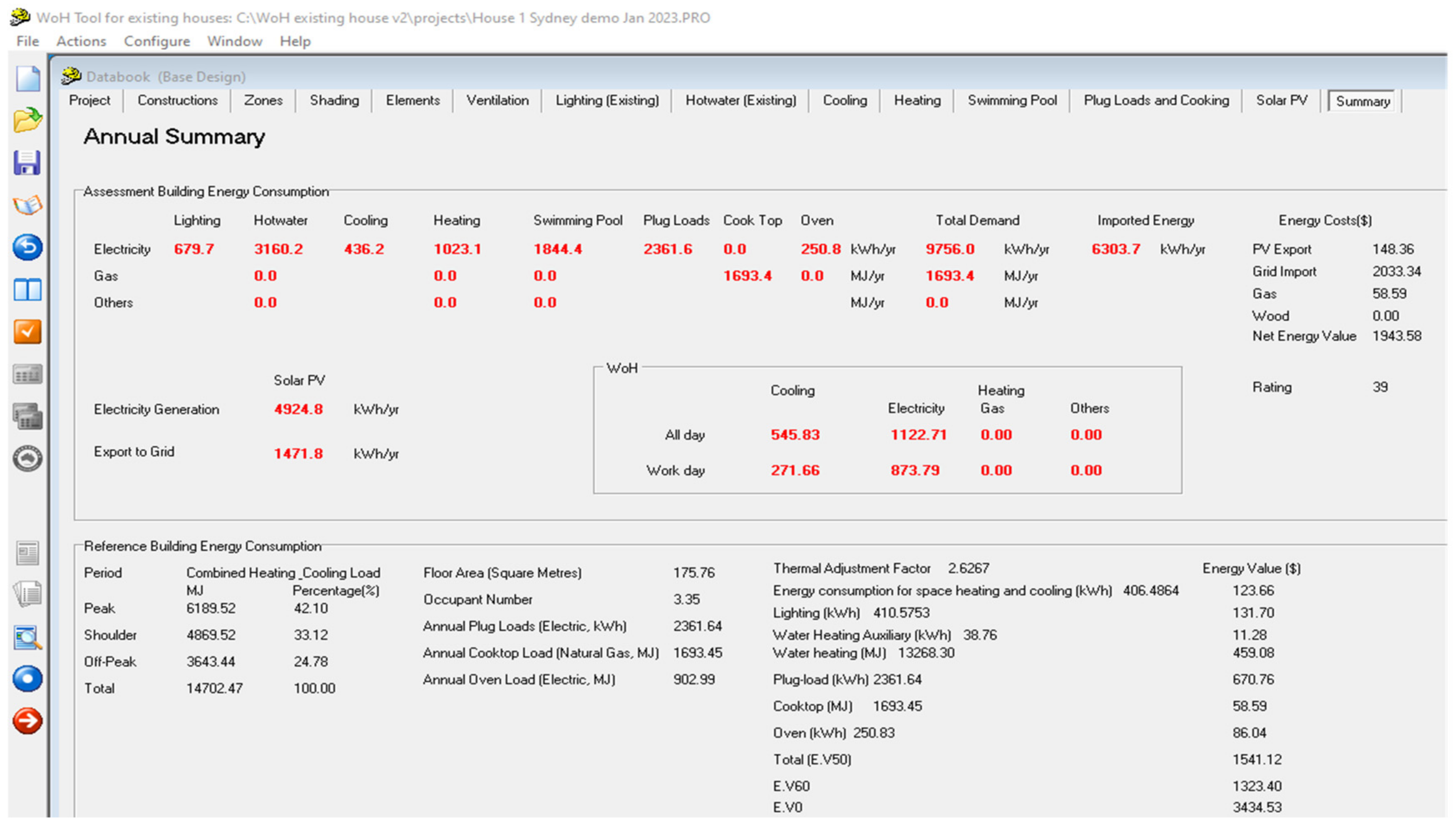
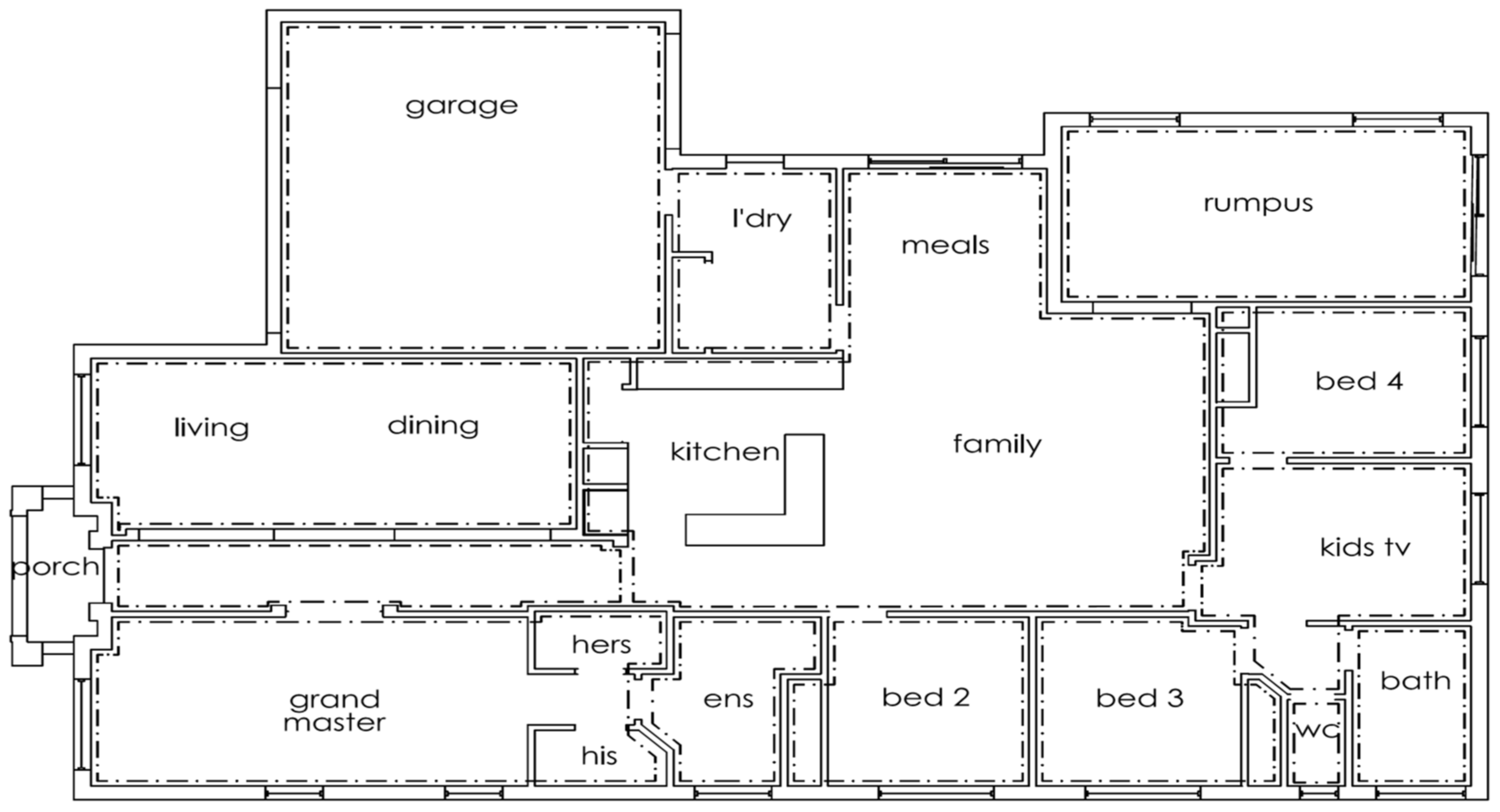
3. Case Study
3.1. Energy Consumption, Energy Value, and Rating
3.2. Retrofitting for Net-Zero Societal Cost Housing
4. Discussions
- Reducing energy demand for space heating and cooling by retrofitting the dwelling building shell to high energy performance;
- Replacing old and low-energy-efficient equipment and appliances with new and high-energy-efficient ones; and
- Installing an on-site renewable energy and battery system.
5. Conclusions
Author Contributions
Funding
Data Availability Statement
Conflicts of Interest
References
- Krarti, M. An overview of artificial intelligence-based methods for building energy systems. J. Sol. Energy Eng. 2003, 125, 331–342. [Google Scholar] [CrossRef]
- Dounis, A. Artificial intelligence for energy conservation in buildings. Adv. Build. Energy Res. 2010, 4, 267–299. [Google Scholar] [CrossRef]
- Zhao, H.; Maoulès, F. A review on the prediction of building energy consumption. Renew. Sustain. Energy Rev. 2012, 16, 3586–3592. [Google Scholar] [CrossRef]
- Gonzalo, F.; Santamaria, B.; Burgos, M. Assessment of Building Energy Simulation Tools to Predict Heating and Cooling Energy Consumption at Early Design Stages. Sustainability 2023, 15, 1920. [Google Scholar] [CrossRef]
- EnergyPlus. Available online: https://energyplus.net (accessed on 4 October 2023).
- ESP-r. Available online: https://www.esru.strath.ac.uk/applications/esp-r/ (accessed on 4 October 2023).
- RETScreen. Available online: https://natural-resources.canada.ca/maps-tools-and-publications/tools/modelling-tools/retscreen/7465 (accessed on 4 October 2023).
- TRANSYS. Available online: https://www.trnsys.com/ (accessed on 5 October 2023).
- HOMER. Available online: https://www.homerenergy.com/ (accessed on 4 October 2023).
- Sefaira. Available online: https://support.sefaira.com/hc/en-us/articles/204769499-Product-Updates-and-Release-Notes (accessed on 4 October 2023).
- BuildSimHub. Available online: https://www.energy.gov/eere/buildings/articles/buildsimhub-brings-github-building-energy-simulation (accessed on 4 October 2023).
- Honeybee. Available online: https://www.ladybug.tools/honeybee.html (accessed on 4 October 2023).
- gEnergy. Available online: https://greenspacelive.com/site/products/genergy/ (accessed on 4 October 2023).
- FineGREEN. Available online: https://www.bimgeneration.com.au/shop/finegreen/ (accessed on 4 October 2023).
- Autodesk Insight. Available online: https://www.autodesk.com/products/insight/overview (accessed on 4 October 2023).
- Autodesk Green Building Studio. Available online: https://gbs.autodesk.com/gbs (accessed on 4 October 2023).
- ResStock. Available online: https://resstock.nrel.gov/ (accessed on 4 October 2023).
- EFEN. Available online: https://getwinpcsoft.com/EFEN-1115872/ (accessed on 4 October 2023).
- Simergy. Available online: https://d-alchemy.com/products/simergy (accessed on 4 October 2023).
- Ali, M.; Prakash, K.; Macana, C.; Bashir, A.; Jolfaei, A.; Bokhari, A.; Klemeš, J.; Pota, H. Modeling residential electricity consumption from public demographic data for sustainable cities. Energies 2022, 15, 2163. [Google Scholar] [CrossRef]
- Nationwide House Energy Rating Scheme (NatHERS), NatHERS Whole of Home National Calculations Method. Available online: https://www.nathers.gov.au/publications (accessed on 16 July 2023).
- Ren, Z.; Jian, A.; Law, A.; Godhani, A.; Chen, D. Development of a benchmark tool for whole of home energy rating for Australian new housing. Energy Build. 2023, 285, 112921. [Google Scholar] [CrossRef]
- Residential Efficiency Scorecard. Available online: http://www.homescorecard.gov.au (accessed on 16 July 2023).
- Ren, Z.; Foliente, G.; Chan, W.; Chen, D.; Ambrose, M.; Paevere, P. A model for predicting household end-use energy consumption and greenhouse gas emissions in Australia. Int. J. Suitable Build. Technol. Urban Dev. 2013, 4, 210–228. [Google Scholar] [CrossRef]
- Ren, Z.; Chen, D.; James, M. Evaluation of a whole-house energy simulation tool against measured data. Energy Build. 2018, 171, 116–130. [Google Scholar] [CrossRef]
- Walsh, P.; Delsante, A. Calculation of the thermal behaviour of multi-zone buildings. Energy Build. 1983, 5, 231–242. [Google Scholar] [CrossRef]
- Ren, Z.; Chen, D. Enhanced air flow modelling for AccuRate—A nationwide house energy rating tool. Build. Environ. 2010, 45, 1276–1286. [Google Scholar] [CrossRef]
- Australian Building Codes Board (2019), Energy Efficiency—NCC 2022 and Beyond Scoping Study. Available online: https://consultation.abcb.gov.au/engagement/energy-efficiency-scoping-study-2019/ (accessed on 16 July 2023).
- Chen, D. Infiltration Calculations in AccuRate (V2.0.2.13). CSIRO Report Submitted to NatHERS. Available online: http://www.nathers.gov.au (accessed on 16 July 2023).
- AS/NZS4234; Heated Water Systems—Calculation of Energy Consumption. Standards Australia: Sydney, Australia, 2008.
- Sustainability Victoria. Comprehensive Energy Efficiency Retrofits to Existing Victorian Houses. Available online: https://www.sustainability.vic.gov.au/research-data-and-insights/research/research-reports/households-retrofit-trials (accessed on 16 July 2023).
- Ren, Z.; Paevere, P.; McNamara, C. A local-community-level, physically-based model of end-use energy consumption by Australian housing stock. Energy Policy 2012, 49, 586–596. [Google Scholar] [CrossRef]
- Ren, Z.; Chen, D.; Wang, X. Climate change adaptation pathways for Australian residential buildings. Build. Environ. 2011, 46, 2398–2412. [Google Scholar] [CrossRef]

| Insulation Description | R-Value (m2.K/W) |
|---|---|
| No document is available on when the building was built. | 0 |
| The building was built before the insulation regulation was introduced in 1991. | 0 |
| The building was built after 1991 and before 2004 with a timber floor. | R1.5 |
| The building was built after 1991 and before 2004 with a slab floor (foil insulation assumed). | R0.85 |
| The building was built between 2004 and 2010. | R1.5 |
| The building was built after 2010. | R2.0 |
| Insulation Description | R-Value (m2.K/W) |
|---|---|
| No document is available on when the building was built. | 0 |
| Foil insulation | R0.75 |
| The building was built before the insulation regulation was introduced in 1991. | R1.5 |
| The building was built between 1991 and 2003. | R2.2 |
| The building was built after the introduction of 5-star in 2004 and before 2009. | R3.0 |
| The building was built after the introduction of 6-star in 2010. | R3.5 |
| Insulation Description | R-Value (m2.K/W) |
|---|---|
| No document on when the building was built | 0 |
| Insulated with foil (standard reflective and concertina foil) | R0.75 |
| Insulated with board (rigid bulk insulation products such as polystyrene) | R1.5 |
| Insulated with batt (glass wool, rockwool, natural wool or polyester) | R1.5 |
| Insulation Product | R Value (m2.K/W) for Measured Thickness (mm) | ||||||
|---|---|---|---|---|---|---|---|
| 1 | 1.5 | 2 | 2.5 | 3 | 3.5 | 4 | |
| Cellulose fibre | 40 | 60 | 80 | 100 | 120 | 140 | 160 |
| Glass fibre | 57 | 86 | 114 | 143 | 165 | 190 | 210 |
| Polyethylense foam | 40 | 60 | 80 | 100 | 120 | 140 | 160 |
| Polyester | 63 | 95 | 126 | 158 | 185 | 210 | 235 |
| Polystyrene (expanded) | 39 | 59 | 78 | 98 | 117 | 137 | 156 |
| Polystyrene (excluded) | 28 | 42 | 56 | 70 | 84 | 98 | 112 |
| Polyurethane rigid foam | 28 | 42 | 56 | 70 | 84 | 98 | 112 |
| Rockwool loose fill | 40 | 60 | 80 | 100 | 120 | 140 | 160 |
| Rockwool batt | 33 | 50 | 66 | 83 | 99 | 116 | 132 |
| Wool loose fill | 80 | 120 | 160 | 200 | 240 | 280 | 320 |
| Wool/polyester batt | 59 | 89 | 118 | 148 | 177 | 207 | 236 |
| On (O’Clock Time) | Off (O’Clock Time) | |
|---|---|---|
| Occupied all day | 0 | 24 |
| Unoccupied during the day | 18 | 7 |
| NatHERS Climate Zone | Average Temperature (°C) | COPadj |
|---|---|---|
| 1 | 27.7 | 0.533 |
| 2 | 26.1 | 0.525 |
| 3 | 24.0 | 0.502 |
| 4 | 21.7 | 0.463 |
| 5 | 24.3 | 0.505 |
| 6 | 21.2 | 0.451 |
| 7 | 22.5 | 0.478 |
| 8 | 19.0 | 0.398 |
| 9 | 20.1 | 0.427 |
| 10 | 20.1 | 0.426 |
| 11 | 18.6 | 0.385 |
| 12 | 19.6 | 0.414 |
| 13 | 18.3 | 0.377 |
| 14 | 13.5 | 0.203 |
| 15 | 17.5 | 0.353 |
| 16 | 17.2 | 0.344 |
| 17 | 18.6 | 0.385 |
| 18 | 16.3 | 0.314 |
| 19 | 20.9 | 0.446 |
| 20 | 15.4 | 0.279 |
| 21 | 15.1 | 0.268 |
| 22 | 13.7 | 0.210 |
| 23 | 12.8 | 0.172 |
| 24 | 13.1 | 0.183 |
| 25 | 8.5 | -0.045 |
| 26 | 12.7 | 0.167 |
| 27 | 17.1 | 0.339 |
| 28 | 16.9 | 0.335 |
| 29 | 26.8 | 0.529 |
| 30 | 29.9 | 0.534 |
| 31 | 26.3 | 0.526 |
| 32 | 24.8 | 0.512 |
| 33 | 26.7 | 0.529 |
| 34 | 24.4 | 0.507 |
| 35 | 22.8 | 0.484 |
| 36 | 22.6 | 0.479 |
| 37 | 26.7 | 0.529 |
| 38 | 26.1 | 0.525 |
| 39 | 24.8 | 0.512 |
| 40 | 24.4 | 0.507 |
| 41 | 23.0 | 0.486 |
| 42 | 22.2 | 0.472 |
| 43 | 21.9 | 0.467 |
| 44 | 18.4 | 0.381 |
| 45 | 19.2 | 0.404 |
| 46 | 18.5 | 0.382 |
| 47 | 16.6 | 0.323 |
| 48 | 16.6 | 0.323 |
| 49 | 15.9 | 0.300 |
| 50 | 18.4 | 0.379 |
| 51 | 18.0 | 0.367 |
| 52 | 18.3 | 0.377 |
| 53 | 16.9 | 0.332 |
| 54 | 18.1 | 0.370 |
| 55 | 16.5 | 0.319 |
| 56 | 17.6 | 0.358 |
| 57 | 15.0 | 0.265 |
| 58 | 15.0 | 0.266 |
| 59 | 11.3 | 0.103 |
| 60 | 14.2 | 0.232 |
| 61 | 13.4 | 0.196 |
| 62 | 14.0 | 0.223 |
| 63 | 13.0 | 0.181 |
| 64 | 27.7 | 0.533 |
| 65 | 11.3 | 0.099 |
| 66 | 12.7 | 0.166 |
| 67 | 13.5 | 0.204 |
| 68 | 11.5 | 0.112 |
| 69 | 9.6 | 0.015 |
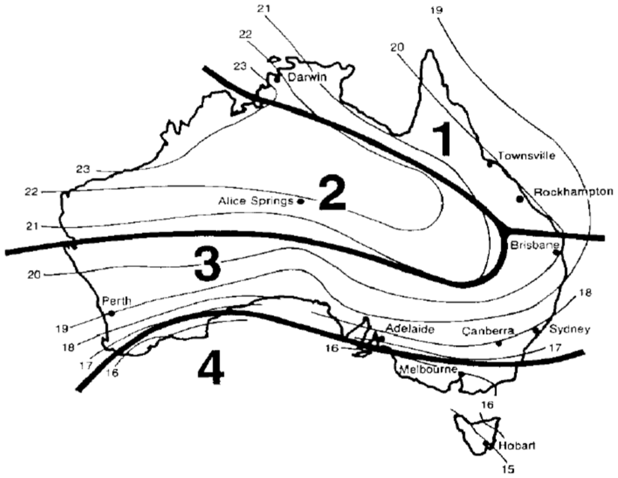
| Hot Water Climate Region | Existing Climate Zones in AccuRate |
|---|---|
| One | 1, 3, 5, 7, 19, 29, 32, 35, 36 |
| Two | 2, 4, 6, 30, 31, 33, 34, 37, 38, 39, 40, 41 |
| Three | 8, 9, 10, 11, 12, 13, 14, 15, 16, 17, 18, 20, 24, 25, 27, 28, 42, 43, 44, 45, 46, 47, 48, 49, 50, 51, 52, 53, 54, 56, 57, 59, 65, 69 |
| Four | 21, 22, 23, 26, 55, 58, 60, 61, 62, 63, 64, 66, 67, 68 |
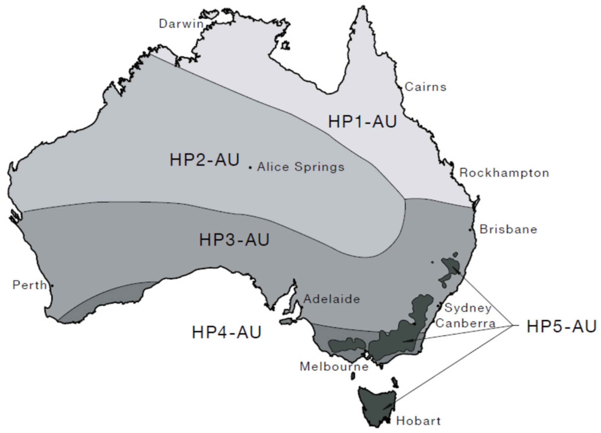
| Month | Hot Water Demand (%) | ||||
|---|---|---|---|---|---|
| Zone 1 | Zone 2 | Zone 3 | Zone 4 | HP5-AU | |
| January | 7.23 | 8.36 | 7.52 | 7.49 | 7.50 |
| February | 7.46 | 8.11 | 7.76 | 7.73 | 7.74 |
| March | 8.51 | 8.75 | 8.66 | 8.66 | 9.32 |
| April | 8.22 | 8.06 | 8.25 | 8.28 | 8.70 |
| May | 8.49 | 7.65 | 8.39 | 8.29 | 9.09 |
| June | 7.99 | 7.31 | 8.02 | 8.12 | 8.53 |
| July | 8.26 | 7.26 | 8.11 | 8.23 | 8.18 |
| August | 8.47 | 7.72 | 8.28 | 8.55 | 8.18 |
| September | 8.88 | 8.53 | 8.55 | 8.62 | 8.21 |
| October | 9.23 | 9.51 | 9.21 | 9.03 | 8.22 |
| November | 8.99 | 9.49 | 8.88 | 8.66 | 8.16 |
| December | 8.26 | 9.26 | 8.37 | 8.35 | 8.18 |
| Water Heater Type | Heating Schedule |
|---|---|
| Solid fuel (f) | Additional research required |
| Off-peak electric (e) | Overnight |
| Continuous electric (e) | Time of use |
| Solar thermal standard efficiency (e) | Additional research required |
| Solar thermal instant gas (g) | Time of use |
| Heat pump (e) | Daytime |
| Gas storage (g) | Time of use |
| Gas instant (g) | Time of use |
| Hour | Time of Use | Daytime | Overnight |
|---|---|---|---|
| 1 | 0 | 0 | 0.25 |
| 2 | 0 | 0 | 0.25 |
| 3 | 0 | 0 | 0.25 |
| 4 | 0 | 0 | 0.25 |
| 5 | 0 | 0 | 0 |
| 6 | 0 | 0 | 0 |
| 7 | 0 | 0 | 0 |
| 8 | 0.15 | 0 | 0 |
| 9 | 0.15 | 0.125 | 0 |
| 10 | 0 | 0.125 | 0 |
| 11 | 0 | 0.125 | 0 |
| 12 | 0.1 | 0.125 | 0 |
| 13 | 0 | 0.125 | 0 |
| 14 | 0.1 | 0.125 | 0 |
| 15 | 0 | 0.125 | 0 |
| 16 | 0.125 | 0.125 | 0 |
| 17 | 0.125 | 0 | 0 |
| 18 | 0.125 | 0 | 0 |
| 19 | 0.125 | 0 | 0 |
| 20 | 0 | 0 | 0 |
| 21 | 0 | 0 | 0 |
| 22 | 0 | 0 | 0 |
| 23 | 0 | 0 | 0 |
| 24 | 0 | 0 | 0 |
| State/Territory | Pump Energy (kWh) | Chlorinator Energy (kWh) |
|---|---|---|
| Victoria | 1300 | 263 |
| South Australia | 1322 | 281 |
| New South Wales | 1424 | 302 |
| Australian Capital Territory | 1529 | 302 |
| Tasmania | 1238 | 263 |
| Queensland | 1529 | 325 |
| West Australia | 1337 | 302 |
| North Territory | 1529 | 325 |
| Season | Cycles Per Day | On Time |
|---|---|---|
| Swimming | 1.5 | 8 am |
| Non-swimming | 1 | 8 am |
| Month | Season |
|---|---|
| January | Swimming |
| February | Swimming |
| March | Swimming |
| April | Swimming |
| May | Non-Swimming |
| June | Non-Swimming |
| July | Non-Swimming |
| August | Non-Swimming |
| September | Non-Swimming |
| October | Swimming |
| November | Swimming |
| December | Swimming |
| Month | Pool Pumping | Number of Hours |
|---|---|---|
| January | 8:00 am–12:30 pm | 4.5 |
| February | 8:00 am–12:30 pm | 4.5 |
| March | 8:00 am–12:30 pm | 4.5 |
| April | 8:00 am–12:30 pm | 4.5 |
| May | 8:00–11:00 am | 3.0 |
| June | 8:00–11:00 am | 3.0 |
| July | 8:00–11:00 am | 3.0 |
| August | 8:00–11:00 am | 3.0 |
| September | 8:00–11:00 am | 3.0 |
| October | 8:00 am–12:30 pm | 4.5 |
| November | 8:00 am–12:30 pm | 4.5 |
| December | 8:00 am–12:30 pm | 4.5 |
| Number of hours for a year | 1413 | |
| Parameters | Societal Energy Costs for Calculations | |||||||
|---|---|---|---|---|---|---|---|---|
| NSW | VIC | QLD | SA | WA | TAS | NT | ACT | |
| Electricity—peak (c/kWh) | 39.80 | 38.41 | 33.46 | 51.29 | 41.24 | 29.96 | 37.32 | 33.88 |
| Electricity—shoulder (c/kWh) | 25.97 | 25.17 | 21.91 | 33.20 | 26.83 | 19.34 | 24.30 | 21.86 |
| Electricity—off-peak (c/kWh) | 20.44 | 19.88 | 17.29 | 25.97 | 21.06 | 15.09 | 19.09 | 17.05 |
| Electricity—controlled load (c/kWh) | 14.07 | 20.61 | 16.74 | 20.43 | 12.73 | 13.50 | 26.90 | 14.83 |
| PV Export (c/kWh) | 10.08 | 13.34 | 11.11 | 11.64 | 7.89 | 9.71 | 26.85 | 9.21 |
| Natural gas (c/MJ) | 3.46 | 2.43 | 4.95 | 4.30 | 4.08 | 3.74 | 3.74 | 3.64 |
| LPG (c/MJ) | 5.58 | 5.58 | 5.58 | 5.58 | 5.58 | 5.58 | 5.58 | 5.58 |
| Wood (c/MJ) | 1.86 | 1.86 | 1.86 | 1.86 | 1.86 | 1.86 | 1.86 | 1.86 |
| Location | Heating (kWh) | Heating Gas (MJ) | Cooling (kWh) | Lighting (kWh) | Hot Water Gas (MJ) | Plug-in (kWh) | Cooktop Gas (MJ) | Oven Gas (MJ) | Total Gas (MJ) | Total Electricity (kWh) |
|---|---|---|---|---|---|---|---|---|---|---|
| Adelaide | 213.7 | 51,972.5 | 1382.3 | 793.2 | 23,323.7 | 2407.1 | 1792.3 | 1904.6 | 78,993.1 | 4796.3 |
| Brisbane | 28.6 | 6949.4 | 2164.4 | 793.2 | 23,323.7 | 2407.1 | 1792.3 | 1904.6 | 33,970 | 5393.3 |
| Canberra | 605.6 | 147,289.9 | 674.7 | 793.2 | 22,969.3 | 2407.1 | 1792.3 | 1904.6 | 173,956.1 | 4480.6 |
| Darwin | 0 | 0 | 17,533.8 | 793.2 | 22,969.3 | 2407.1 | 1792.3 | 1904.6 | 26,666.2 | 20,734.1 |
| Hobart | 646.5 | 157,254.9 | 25.3 | 793.2 | 23,618.5 | 2407.1 | 1792.3 | 1904.6 | 184,570.3 | 3872.1 |
| Melbourne | 273 | 66,396.6 | 835.9 | 793.2 | 24,353.7 | 2407.1 | 1792.3 | 1904.6 | 94,447.2 | 4309.2 |
| Perth | 140.6 | 34,192 | 2019.1 | 793.2 | 23,618.5 | 2407.1 | 1792.3 | 1904.6 | 61,507.4 | 5360 |
| Sydney | 110.5 | 26,877.2 | 1093.3 | 793.2 | 24,353.7 | 2407.1 | 1792.3 | 1904.6 | 54,927.8 | 4404.1 |
| Location | Heating (kWh) | Cooling (kWh) | Lighting (kWh) | Hot Water (kWh) | Plug-In (kWh) | Cooktop (kWh) | Oven (kWh) | Total Electricity (kWh) | Ratio of Electricity Use for Space H/C to Total Electricity |
|---|---|---|---|---|---|---|---|---|---|
| Adelaide | 3125.1 | 1382.3 | 793.2 | 2789 | 2407.1 | 322.6 | 265.5 | 11,084.8 | 40.7 |
| Brisbane | 446.9 | 2164.4 | 793.2 | 3857.4 | 2407.1 | 322.6 | 265.5 | 10,257.1 | 25.5 |
| Canberra | 9462.8 | 674.7 | 793.2 | 2907.8 | 2407.1 | 322.6 | 265.5 | 16,833.7 | 60.2 |
| Darwin | 0 | 17,533.8 | 793.2 | 2907.8 | 2407.1 | 322.6 | 265.5 | 24,230 | 72.4 |
| Hobart | 10,112.4 | 25.3 | 793.2 | 2907.8 | 2407.1 | 322.6 | 265.5 | 16,833.9 | 60.2 |
| Melbourne | 4269.7 | 835.9 | 793.2 | 2837.4 | 2407.1 | 322.6 | 265.5 | 11,731.4 | 43.5 |
| Perth | 2055.9 | 2019.1 | 793.2 | 2789 | 2407.1 | 322.6 | 265.5 | 10,652.4 | 38.3 |
| Sydney | 1616.1 | 1093.3 | 793.2 | 2718.1 | 2407.1 | 322.6 | 265.5 | 9215.9 | 29.4 |
| Location | Grid Imported (kWh) | Grid Imported (A$) | Gas Value (A$) | Net Energy Value (A$) | Energy Rating Scale |
|---|---|---|---|---|---|
| Adelaide | 4796.3 | 1869.3 | 2393.8 | 4263.1 | 14 |
| Brisbane | 5393.2 | 1376.2 | 527 | 1903.2 | 48 |
| Canberra | 4480.6 | 1140.6 | 5495.8 | 6636.6 | 0 |
| Darwin | 20,734.2 | 5929.7 | 138.3 | 6067.9 | 6 |
| Hobart | 3872.1 | 857.9 | 6019.6 | 6877.5 | 0 |
| Melbourne | 4309.2 | 1256.6 | 1703.3 | 2959.9 | 6 |
| Perth | 5359.9 | 1699 | 1545.9 | 3244.8 | 22 |
| Sydney | 4404.1 | 1317.5 | 1057.9 | 2375.3 | 34 |
| Location | Grid Imported (kWh) | Net Energy Value (A$) | Energy Rating Scale |
|---|---|---|---|
| Adelaide | 11,085 | 4373.5 | 13 |
| Brisbane | 10,257 | 2640.8 | 34 |
| Canberra | 16,833.9 | 4394.9 | 0 |
| Darwin | 24,229.5 | 6953.9 | 0 |
| Hobart | 16,834.5 | 3884 | 0 |
| Melbourne | 11,731.4 | 3481.9 | 0 |
| Perth | 10,653 | 3385.7 | 20 |
| Sydney | 9215.9 | 2804.7 | 26 |
| Location | Heating (kWh) | Cooling (kWh) | Lighting (kWh) | Hot Water (kWh) | Plug-in (kWh) | Cooktop (kWh) | Oven (kWh) | Total Electricity (kWh) | Electricity Saving (%) |
|---|---|---|---|---|---|---|---|---|---|
| Adelaide | 433.5 | 263.4 | 654.5 | 650 | 2407.1 | 322.6 | 265.5 | 4996.6 | 54.9 |
| Brisbane | 20.1 | 456.7 | 654.5 | 172.5 | 2407.1 | 322.6 | 265.5 | 4299.0 | 58.1 |
| Canberra | 1590.6 | 94.4 | 654.5 | 570 | 2407.1 | 322.6 | 265.5 | 5912.7 | 64.9 |
| Darwin | 0 | 3833.8 | 654.5 | 134.7 | 2407.1 | 322.6 | 265.5 | 7618.2 | 68.6 |
| Hobart | 1680.1 | 2 | 654.5 | 1057.9 | 2407.1 | 322.6 | 265.5 | 6389.7 | 62.0 |
| Melbourne | 609 | 165.5 | 654.5 | 890.6 | 2407.1 | 322.6 | 265.5 | 5314.8 | 54.7 |
| Perth | 221.5 | 373.2 | 654.5 | 362.2 | 2407.1 | 322.6 | 265.5 | 4606.6 | 56.8 |
| Sydney | 170.2 | 220 | 654.5 | 528.8 | 2407.1 | 322.6 | 265.5 | 4568.7 | 50.4 |
| Location | PV Size (kW) | PV Generation (kWh) | Total Electricity Demand (kWh) | PV Exported (kWh) | PV Exported (A$) | Grid Imported (kWh) | Grid Imported (A$) | Net Energy (kWh) | Net Energy Value (A$) | Energy Rating Scale |
|---|---|---|---|---|---|---|---|---|---|---|
| Adelaide | 3.5 | 5577.1 | 4996.6 | 3570.6 | 415.6 | 2990.3 | 1175.8 | 580.3 | 760.2 | 85 |
| Brisbane | 3.0 | 5144.1 | 4299.0 | 3459.9 | 384.4 | 2614.7 | 681.9 | 845.2 | 297.5 | 91 |
| Canberra | 4.0 | 6507.7 | 5912.7 | 4318.3 | 397.7 | 3723 | 975.4 | 595.3 | 577.7 | 85 |
| Darwin | 5.0 | 8430.4 | 7618.2 | 5736.7 | 1540.3 | 4924.5 | 1359.1 | 812.2 | −181.2 | 103 |
| Hobart | 5.0 | 6667.2 | 6389.7 | 4267.6 | 414.4 | 3990.3 | 927.5 | 277.3 | 513.1 | 85 |
| Melbourne | 4.0 | 5661.3 | 5314.8 | 3536.5 | 471.8 | 3190 | 947.5 | 346.5 | 475.7 | 86 |
| Perth | 3.0 | 5010.9 | 4606.6 | 3208.7 | 253.2 | 2804.6 | 891.2 | 404.1 | 638 | 85 |
| Sydney | 3.5 | 5320 | 4568.7 | 3468.3 | 349.6 | 2716.8 | 838.9 | 751.5 | 489.3 | 87 |
Disclaimer/Publisher’s Note: The statements, opinions and data contained in all publications are solely those of the individual author(s) and contributor(s) and not of MDPI and/or the editor(s). MDPI and/or the editor(s) disclaim responsibility for any injury to people or property resulting from any ideas, methods, instructions or products referred to in the content. |
© 2023 by the authors. Licensee MDPI, Basel, Switzerland. This article is an open access article distributed under the terms and conditions of the Creative Commons Attribution (CC BY) license (https://creativecommons.org/licenses/by/4.0/).
Share and Cite
Ren, Z.; Jian, A.; Chen, D. Development of an Energy Rating Tool for Australian Existing Housing. Energies 2023, 16, 7368. https://doi.org/10.3390/en16217368
Ren Z, Jian A, Chen D. Development of an Energy Rating Tool for Australian Existing Housing. Energies. 2023; 16(21):7368. https://doi.org/10.3390/en16217368
Chicago/Turabian StyleRen, Zhengen, Ai Jian, and Dong Chen. 2023. "Development of an Energy Rating Tool for Australian Existing Housing" Energies 16, no. 21: 7368. https://doi.org/10.3390/en16217368
APA StyleRen, Z., Jian, A., & Chen, D. (2023). Development of an Energy Rating Tool for Australian Existing Housing. Energies, 16(21), 7368. https://doi.org/10.3390/en16217368