Research on Full Premixed Combustion and Emission Characteristics of Non-Electric Gas Boiler

Abstract

NO_x has become one of the main culprits causing the global greenhouse effect, and excessive emissions of NO_x can also cause some common diseases in humans. The denitrification of power plant boilers has been 100% popularized, and their denitrification efficiency has reached national and local environmental requirements (such as Selective Catalytic Reduction, SCR). However, small gas boilers, due to their use of relatively clean fuels, have relatively low NO_x emissions. But, local environmental protection departments have weak supervision of small clean fuel boilers, and these equipment generally lack specialized denitrification equipment, resulting in NO_x emissions still not meeting standards. In addition, there are many small gas boilers, resulting in high total emissions. The fully premixed burner of a small gas boiler has the effect of suppressing NO_x production during combustion. This study designed a surface porous burner with different combustion intensities at different positions. The experimental results and numerical calculations show that for horizontal combustion, the burner has different intake rates at different axial positions, enabling uniform combustion throughout the entire furnace, with NO_x emissions below 30 mg/Nm³. The numerical simulation results show that the NO_x emissions are 26.6 mg/m³. The calculated results are in good agreement with the actual situation. The generation of NO_x is mainly thermal, with a maximum error of 15.4% between the calculated and experimental values. The difference between the calculated value of O and the experimental one is 5.1%. It can be seen that numerical simulation has considerable accuracy.

1. Introduction

Sustained economic growth brings about the rapid growth of energy demand, but the massive use of traditional energy such as coal, oil, etc. means that people must face the serious threat of global warming, thus accelerating people’s demand for clean energy and other non-fossil energy. The Paris climate agreement requires that the emissions of CO₂ and other greenhouse gases should be close to zero by 2100 [1,2,3,4]. However, at this stage, the energy structure is still dominated by coal, and other clean energy sources such as natural gas can only be used as auxiliary energy due to high prices and imperfect basic transportation facilities. Hence, it is very difficult to achieve zero greenhouse gas emissions in the short term [5,6].

Given the high price of natural gas and its low carbon emissions, advanced denitrification measures have been adopted for boilers in service or under construction to reduce NO_x while ensuring that other harmful gases to the environment and human health do not exceed the standard, including CO, SO₂, etc. These gases can damage the ozone layer and cause great harm to human health [7,8]. Moreover, with the increasing improvement of China’s environmental protection standards, the limits on NO_x emission values in the Beijing-Tianjin-Hebei region are becoming more and more stringent [9]. The NO_x emission value of new boilers in the mentioned region from April 2017 should not be higher than 30 mg/Nm³. Although natural gas itself is a clean fuel, its use in gas-fired boilers requires the consideration of low NO_x emissions. For this reason, scholars have also conducted extensive research. Denitration technology is generally divided into the following three categories according to its characteristics: pre-treatment, combustion denitration, and flue gas post-treatment denitration [10]. Among the three methods, the first method is less used, the second method makes it easy to reduce the boiler thermal efficiency and increase the carbon content of fly ash, and the third denitrification method is widely used, but it has major defects such as a large land area, complex system, and high investment cost [11].

Scholars have carried out fruitful research on the denitration of flue gas and have accomplished a number of academic achievements and demonstrated an excellent denitration effect. Nhan et al. [12] used internal flue gas recirculation combustion equipment to reduce NO_x emissions in medium-sized boilers. The main principle was to set up internal flue gas recirculation channels on the basis of the original combustion device, and even if a small amount of recirculated flue gas is led to the root of the combustion flame, a good denitrification effect can be achieved. Under certain operating conditions, the NO_x emission is reduced from 82.83 ppm to 9.7 ppm. Son et al. [10] developed a post-treatment method to absorb and transform NO_x at low temperature, and its reaction temperature can be as low as 298 K compared with SCR (Selective Catalytic Reduction) or SNCR (Selective non-Catalytic Reduction) methods. Yu et al. [13] compared the combustion characteristics and emission characteristics of porous media surface burners and concluded that porous metal media surface burners had superior performance compared with ceramic and stainless steel, and the optimal equivalent ratio in the experimental range was 0.8. Matsumoto et al. [14] used dimethyl reburning and flue gas recirculation technology to reduce NO_x emissions. The experiment proved that under optimal working conditions, NO_x emissions could be reduced to 13 ppm, which was 9% of that without FGR (internal flue gas recirculation), and it was an economical and effective denitrification measure. Habib et al. [15] studied the relationship between combustion conditions in the furnace and the average temperature, maximum temperature, and NO emission value through numerical simulation. For a given flue gas flow rate, the average temperature and NO concentration in the furnace increased with the increase in excess air coefficient. When the amount of fuel is constant and the excess air coefficient value is 1.2, the maximum NO emission occurs at the furnace outlet. When the combustion temperature increases, the thermal type NO in the furnace will increase sharply. When the swirl angle is 45°, the NO emission can be minimized. Shalaj et al. [16,17] studied the influence of fins installed in the furnace on the temperature field and NO_x emissions in the furnace in 2015. The addition of fins can enhance the convection heat transfer in the furnace, enhance the flue gas reflux, and reduce the NO_x emission at the furnace outlet. In 2016, a numerical calculation was used to study the effects of mixed combustion gas recirculation on the maximum temperature and NO emission in the furnace. It was concluded that with the increase in recirculation rate (0–1), the maximum temperature in the furnace decreased from 1995 °C to 1920 °C, and the maximum NO value was positively correlated with the maximum temperature in the furnace, and the maximum emission appeared at r = 0. This study is consistent with the conclusion reached by Nhan et al. [12].

The use of flue gas recirculation for denitrification has also achieved good research results. Whether it is FGR or EFGR (external flue gas recirculation), the flue gas recirculation volume is strictly limited and the optimal circulation volume is limited between 10 and 20% under most working conditions. Insufficient flue gas recirculation volume leads to a poor denitrification effect. Excessive flue gas circulation will cause combustion instability [18]. Although the denitrification effect in the use of FGR and EFGR has been confirmed by the above experiments and numerical calculations, the technology itself makes certain changes to the burner or boiler body (such as adding external circulation pipes and control facilities), resulting in a higher investment and more complex control systems. As the requirements of denitrification cost and denitrification effect become more and more strict, the full premixed burner is paid more and more attention. The full premixed technology is generally only changed on the burner, so its denitrification cost is greatly reduced compared with external gas recirculation. On the other hand, the full premixed combustion can increase the flame filling degree so that the furnace temperature distribution is more uniform and the boiler size is more compact. The recovery of low-temperature heat in condensing boilers has strict requirements on the heating surface layout, so the full premixed combustion mode is widely used in condensing boilers [19,20]. Further, to achieve thin surface combustion, the burners are mostly made of ceramic and metal fibers [4,21,22,23,24,25]. Bouma et al. [22] used a one-dimensional numerical simulation to study fully premixed combustion, taking into account the influence of heat transfer between gas and the ceramic surface of the burner, as well as the radiation heat transfer of ceramic materials in the calculation process. Compared with the experimental value, the NO_x emission error is within the acceptable range. Ignoring the gas radiation heat transfer will lead to greater calculation error, which has little effect on the flame temperature but has a greater effect on the downstream flue gas. Malico et al. [23] established a two-dimensional model and solved the N-S equation to calculate and predict CO and NO_x emissions: the predicted values of CO emissions were low while the predicted values of NO_x emissions were high. Lee et al. [26] studied the influence of the distance between the outlet of the fully premixed burner and the premixed flame on the emission of NO and CO. To this end, the heat exchanger and the flue gas flow space were modified and adjusted, and the heat exchanger was divided into two groups in the direction of the flue gas flow. The distance between the burner outlet and the first group of heat exchangers was L₁, and the distance between the first group and the second group of heat exchangers was L₂. In general, the amount of NO decreases with the decrease in L₁, while the amount of CO increases. When L₂ increases, the amount of CO produced increases, while the amount of NO produced changes little, so L₁ determines the amount of NO produced and L₂ determines the amount of CO produced. Pil Hyong Lee et al. [27] analyzed that the lack of mixing process in unpremixed burners leads to excessively long combustion flame and a series of problems, such as the uncompact arrangement of the boiler heating surface due to an excessively long flame length, which affects the overall size of the boiler and leads to unstable combustion, etc. Therefore, it is generally recommended to use fully premixed burners for compact condensing boilers. When oxygen is zero and other conditions are optimal, NO emissions are less than 6 ppm, CO emissions are less than 49.1 ppm. With non-premixed burners, it is difficult to achieve thin surface combustion so as to achieve low NO_x emissions. Especially for high-efficiency condensing boilers, it is recommended to use thin surface burners in terms of boiler size, in-furnace temperature equalization, and technology for reducing NO [27,28,29,30,31,32]. The number of condensing boilers continues to grow in China, Europe, and the United States [30,31,33], so the demand for fully premixed surface porous media burners is growing. Through numerical simulation and experimental methods, Hinrichs et al. [20] verified that the lack of combustion front in surface medium combustion resulted in a significant reduction in NO_x emissions, which was due to the large amount of NO produced at the combustion front, while only a small amount of NO was produced behind the front. Currently, there are many studies on low NO_x emissions from coal-fired or power plant boilers [34,35,36,37,38,39,40,41]. However, there is relatively little research on gas industrial boilers. This study draws on the experience of other researchers and has been optimized to design a dedicated burner that can be specifically used for denitrification in gas boilers.

Considering the similarity of the gas boiler and condensing boiler in dimensions and subsequent heating surface, a surface burner is designed for the boiler and the temperature in the furnace and NO and CO emissions in various working conditions are compared through experimental measurements and numerical simulations so as to determine the advantages of this burner in emission reduction.

It provides a theoretical basis for the design of a small, low-NO_x surface gas burner. Based on China’s increasingly strict environmental requirements and stricter local environmental restrictions on NO_x emissions, this study designed a fully premixed low-NO_x burner. On-site experiments and numerical calculations have confirmed that this burner has unique advantages in NO_x reduction and is low-cost and easy to achieve.

Due to the unique advantages of numerical simulations compared to on-site experiments, such as cost and the ability to obtain temperature values under special operating conditions without being constrained by boundary conditions, this study adopts numerical simulation methods for research and compares the calculated results with experimental data to obtain the optimal research results.

2. Low-NO_x Combustion Experiment and Methods

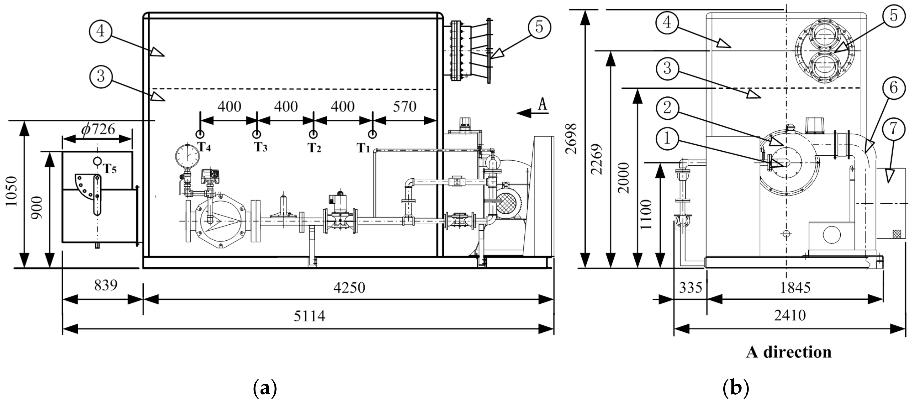
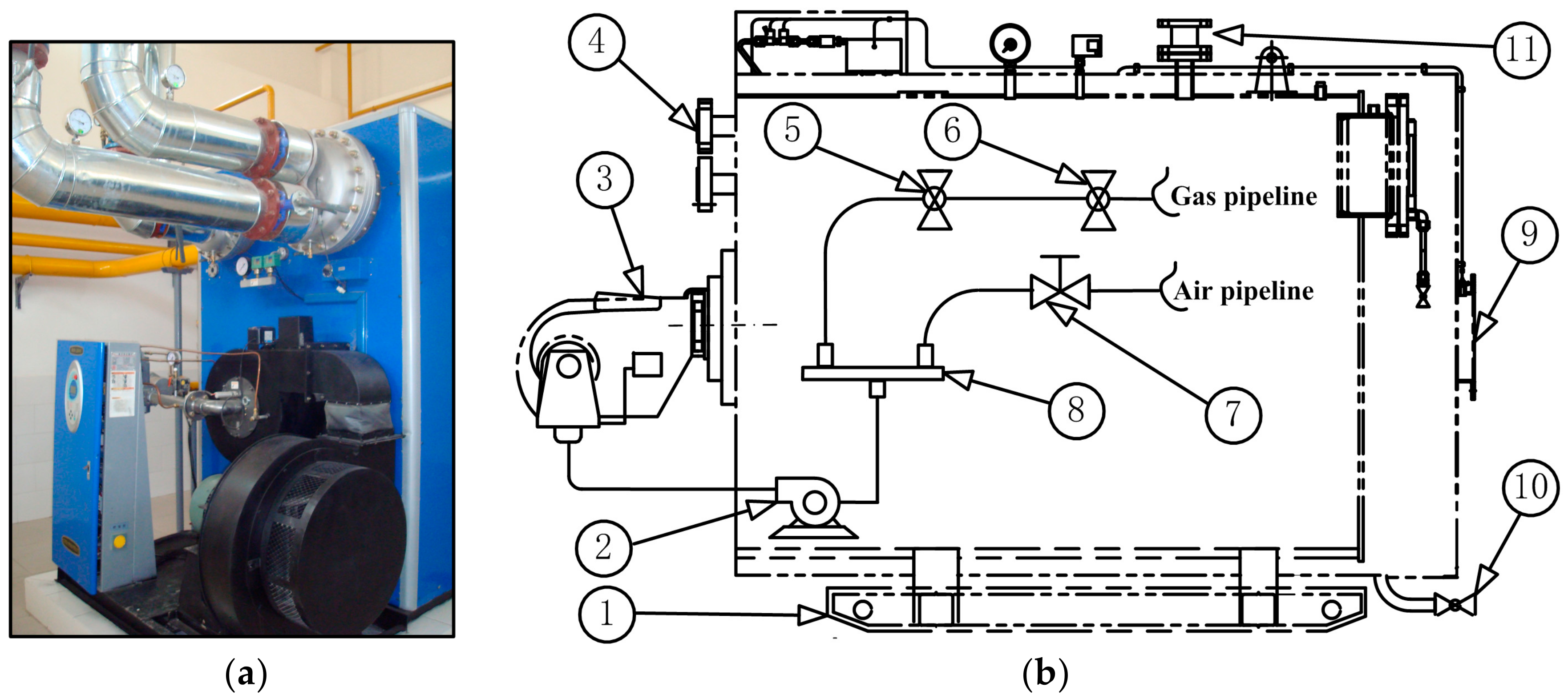
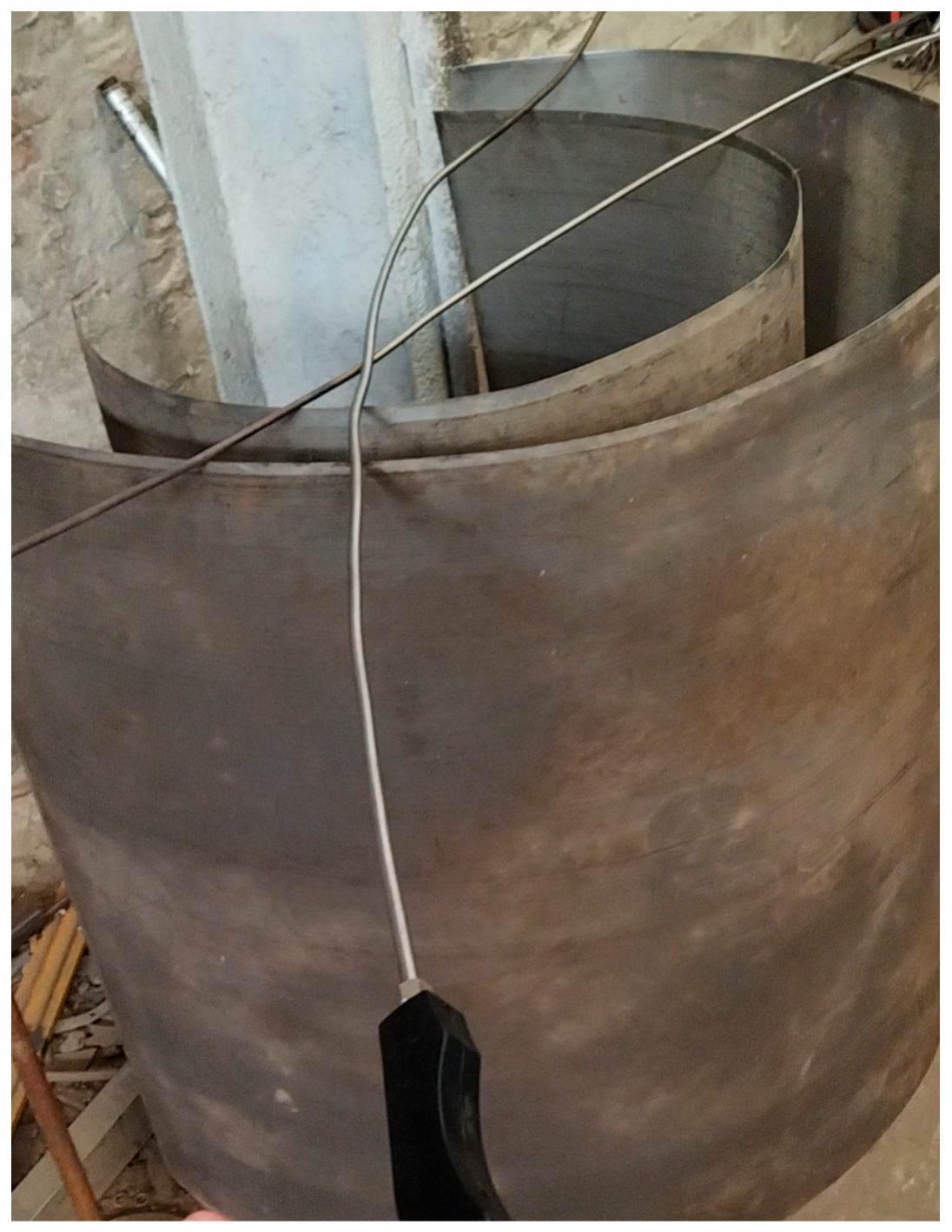
2.1. Experimental Boiler and System

The new low-N surface burner is installed on a horizontal boiler, and the schematic diagram of the boiler is shown in Figure 1. The boiler is a vacuum boiler produced in Japan, providing domestic hot water for a certain automotive 4S store. The boiler and the base are welded as a whole, and the boiler body 3, 4, and accessories are shipped quickly. The main accessories include burner 1, gas and air supply pipeline, chimney 6, blower 7, and vacuum coil heat exchanger 5. The boiler output is 2 t/h, and the boiler accessories are packed with the whole boiler, and the boiler packing size is 5114 × 2410 × 2698 mm. At the height of the furnace 1050 mm and 650 mm away from the front wall of the furnace, four temperature measuring points are arranged at an equal distance of 750 mm, as shown in Figure 1a. At the points T1, T2, T3, and T4, the smoke temperature and components can be measured. A measuring point T5 is arranged at the chimney outlet to measure the exhaust temperature and exhaust component content.

The photos of the experimental furnace body are shown in Figure 2a, and the boiler is placed horizontally on base 1 (shown in Figure 2b). A fully premixed low-nitrogen burner is installed in front of the furnace. In order to evenly mix gas and air, a radial multi-chamber static mixer is equipped in front of the burner, which adopts the dedicated static mixing structure designed by Shi et al. [34]. Since the boiler rate is small and the pressure drop of the whole furnace pipeline is small, blower 2 is arranged behind the static mixer to overcome the pressure drop of the flue gas process. The vacuum boiler is equipped with a set of vacuum coils, and the single circuit heating is shown in part 4 of Figure 2. The gas system is composed of two channels, the gas pipeline and air pipeline. The lowest point at the bottom of the boiler is equipped with drain valve 10, and the top is equipped with vent valve 11. The flue gas (after combustion and heat transferring) enters the chimney through flue gas outlet 9 and is discharged into the atmosphere. The emission of flue gas NO_x and CO here meets the emission requirements of air pollutants in Beijing. The experimental location is a certain automobile 4S store in Shunyi District, Beijing. The composition of natural gas used in the experiment is shown in

Table 1. Natural gas composition table.

Items	CH4	C2H8	C3H8	N2	Density/kg·Nm−3	High Calorific Value/MJ·Nm−3	Lower Calorific Value/MJ·Nm−3
Natural gas	96.15	0.25	0.01	3.59	0.7174	38.47	34.7

. It can be seen that the main component of natural gas used in the experiment is methane (CH₄) and the nitrogen content in the natural gas component is high. Therefore, the denitrification efficiency and monitoring of CO generation during combustion are very important for the economic operation of the boiler and low nitrogen combustion.

2.2. Low-N Surface Combustion Experiment

The interior size of the furnace of the research object is cylindrical, the inner diameter is 1 m, and the depth of the furnace is 2 m. The composition of natural gas is shown in Table 1. The boiler gas flow rate and air flow rate are measured by flow instruments on the pipeline. The model gas flow meter is LWGQ-C with a measurement accuracy of 0.01%, and the model of the air flow meter is KFLUGB with a measurement accuracy of 0.015%. The temperature in the furnace is measured by a DT1320 high-temperature contact tropical electric couple thermometer with a measuring accuracy of 1%. The measurement of flue gas composition adopts an ecom-J2KN type flue gas analyzer, the measurement accuracy of O₂ is 0.2%, the measurement accuracy of CO, NO, NO₂, SO₂ is 5% of the measurement value, the measurement error of smoke temperature is 1% of the measurement value, and the converted oxygen of NO, NO₂, CO measurement value is 3.5%. This type of component analyzer can withstand a maximum temperature of 1200 °C. The experimental results are shown in

Table 2. Industrial experimental data.

Natural Gas		Air Door Angle (%)	Flue Gas						Excess Air Coefficient (α)
Standard Natural Gas Flow (Nm3/h)	Supply Gas Pressure/Kpa		Furnace Pressure/Kpa	O2 (%)	NOx Emission Index (mg/Nm3)	CO Emission Index (ppm)	CO2 Emission Index (ppm)	Exhaust Gas Temperature
80	9	17	−18	5	34.8	229	9.07	82	1.32
90	9	21	−18	4	18.7	60	9.63	108	1.24
150	9	32	−15	5	21.3	48	9.07	138	1.31
160	9	40	−15	4.1	22.6	11	9.58	168	1.24
181	9	45	−15	4.4	23.4	2	10.2	201	1.27
210	9	61	−8	4.2	25.7	2	9.52	206	1.25

.

As can be seen from Table 2, low nitrogen combustion can be achieved by using this type of fully premixed burner, and low NO_x emission can be achieved under all the conditions in the table (NO_x emission value is lower than 30 mg/Nm³) [9]. By adjusting the throttle opening, the CO emission also showed a gradually decreasing trend, indicating that the combustion efficiency of the burner gradually increased under experimental conditions. As the opening of the damper increases, the exhaust temperature of the boiler gradually increases, indicating that with the increase in gas supply, the amount of flue gas in the furnace gradually increases, causing a large amount of flue gas heat generated to enter the chimney and exhaust into the atmosphere before it can be transferred to the thermal medium, resulting in a gradually increasing trend of measured flue gas temperature. The highest exhaust temperature is 206 °C, and the lowest exhaust temperature is 82 °C. The negative pressure inside the furnace gradually decreases, which is due to the increasing amount of gas supply and the opening of the air door, leading to a gradual increase in the amount of flue gas inside the furnace, resulting in a decrease in negative pressure inside the furnace. However, there has been a slight negative pressure phenomenon in the furnace, and there has been no phenomenon of flame spraying from the furnace observation hole during the experiment, ensuring the safety of the boiler during operation. The actual excess air coefficient of the boiler is maintained at 1.24–1.32. In order to comprehensively investigate the combustion characteristics of fully premixed burners and the temperature distribution of the entire furnace, numerical simulation methods were used to calculate the combustion characteristics of this type of burner, while evaluating the NO_x emission status of this type of burner.

The experimental conditions are full scale combustion experiments, which can accurately and comprehensively measure various emission conditions of the boiler, and all indicators of the boiler meet the requirements. In order to comprehensively verify the rationality of the experiment, this study also used numerical simulations to conduct full-scale three-dimensional calculations on the boiler in order to review the experimental data. Therefore, a more detailed analysis of the experimental data is placed in the simulation section for comparison between the two.

3. Numerical Methods

3.1. Numerical Methods and Physical Models

In order to evenly distribute the temperature on the surface of the burner, the mixture of gas and air on each part of the burner surface should be evenly distributed. To achieve uniform distribution of mixed gas in each part, balancing the airflow velocity on the burner surface is crucial. Due to the complexity of the surface flow distribution of porous surface combustion equipment, it is difficult to characterize the complex flow and combustion characteristics of the entire surface of the burner by experimental methods only [13,27]. Therefore, the method of combining numerical simulations and experiments is used in this paper to calculate the flow and combustion in the full-size furnace of a specific surface burner, and the calculated results are compared with the experimental values to verify the accuracy of the calculated ones and supplement the defects of the experiment itself.

Due to the numerous nozzle holes on the porous medium of the surface burner, the complexity of surface combustion is much higher than that of non-premixed combustion. Moreover, compared to the finite rate model of non-premixed combustion, surface combustion takes longer and occupies more memory in solving component transport equations and chemical reaction processes [20]. Compared with non-premixed combustion, the flamelet progress variable model FPV, established for non-premixed combustion, can also be applied to the premixed combustion model because the flame length of premixed combustion is significantly shortened. It is assumed that the length and time scale of the premixed chemical reaction are extremely short [42,43,44].

The flame propagation velocity of premixed combustion depends on the propagation velocity of laminar flames and the coherent effect of turbulence on laminar flames. Vortices in turbulent flow can deform and wrinkle the flame front and then affect the propagation speed of the flame front. Combustion reactants and combustion products in the premix reaction are strictly separated by the flame region. This calculation uses FLUENT 2020 for premix calculations, and only turbulence and subsonic flow can be used. The premix combustion model cannot be used together with the pollutant generation model (NO_x). The combustion reaction simulation uses the Finite-Rate Chemistry Model in FLUENT [45,46].

The premixed combustion model uses the standard k-e model, and the equations are as follows [47,48,49]:

$$\frac{\partial \rho k}{\partial t}+\frac{\partial (\rho k{u}_{\mathrm{i}})}{\partial x_{\mathrm{i}}}=\frac{\partial }{\partial x_{\mathrm{j}}}[(\mu +\frac{{\mu }_{\mathrm{t}}}{{\sigma }_{\mathrm{k}}})\frac{\partial \mathrm{k}}{\partial {\mathrm{x}}_{\mathrm{j}}}]+G_{\mathrm{K}}+G_{\mathrm{b}}-\rho \epsilon -Y_{\mathrm{M}}+S_{\mathrm{K}}$$

(1)

$$\frac{\partial \rho \epsilon }{\partial t}+\frac{\partial (\rho \epsilon u_{\mathrm{i}})}{\partial x_{\mathrm{i}}}=\frac{\partial }{\partial x_{\mathrm{j}}}[(\mu +\frac{{\mu }_{\mathrm{t}}}{{\sigma }_{\epsilon }})\frac{\partial \epsilon }{\partial {\mathrm{x}}_{\mathrm{j}}}]+{\mathrm{C}}_{1\epsilon }\frac{\epsilon }{k}(G_{\mathrm{k}}+{\mathrm{C}}_{3\epsilon }{G}_{\mathrm{b}})-C_{2\epsilon }\rho \frac{{\epsilon }^2}{k}+S_{\epsilon }$$

(2)

In the formula, G_k and G_b represent the average velocity gradient generation term and buoyancy generation term, respectively. Y_M represents the pulsation generation term; C_1ε, C_2ε are constants whose values are 1.44 and 1.92, respectively, and C_3ε is an empirical constant. S_k and S_ε are source terms.

The convection diffusion equation uses the following general form of conservation equation [50]:

$$\frac{\partial }{\partial t}(\rho Y_{\mathrm{i}})+\nabla ·(\rho \overrightarrow{v}{Y}_{\mathrm{i}})=-\nabla ·{\overrightarrow{J}}_{\mathrm{i}}+R_{\mathrm{i}}+S_{\mathrm{i}}$$

(3)

In the formula, R_i is the net generation rate of the i-th component in the chemical reaction, and S_i is the net generation rate obtained by adding diffusion and user-defined source terms. When using a user-defined model, if there are N fluid phase chemical components in the system, it is necessary to solve N − 1 such equations. According to the principle of mass conservation, the sum of the mass fractions of all components is equal to 1, and the mass fraction of the N-th component is obtained by subtracting the N − 1 mass fraction from 1. Therefore, in order to reduce the error, the component with the largest mass should be taken as the N-th component. When the oxidizing agent is air, N₂ is chosen as the N-th component [46].

As shown in Table 1, the main component of natural gas is methane. Based on the above three assumptions, the chemical reaction equation in the furnace is shown in

Table 3. Summary of chemical equations for premixed gas combustion reaction.

Serial Number	Chemical Equations	Rate Exponent	PEF (Pre-Exponential Factor)	AE (Activation Energy)	TE (Temperature Exponent)
1	$\mathrm{C}{\mathrm{H}}_4+1.5{\mathrm{O}}_2\rightleftharpoons \mathrm{CO}+2{\mathrm{H}}_2\mathrm{O}$	$\begin{array}{l}\mathrm{C}{\mathrm{H}}_4=1.46\\ {\mathrm{O}}_2=0.5217\end{array}$	1.6596 × 1015	1.72 × 108
2	$\mathrm{CO}+0.5{\mathrm{O}}_2\rightleftharpoons \mathrm{C}{\mathrm{O}}_2$	$\begin{array}{l}\mathrm{CO}=1.6904\\ {\mathrm{O}}_2=1.57\end{array}$	7.9799 × 1014	9.654 × 107
3	$\mathrm{C}{\mathrm{O}}_2\rightleftharpoons \mathrm{CO}+0.5{\mathrm{O}}_2$	$\mathrm{C}{\mathrm{O}}_2=1$	2.2336 × 1014	5.1774 × 108
4	${\mathrm{N}}_2+{\mathrm{O}}_2+0\mathrm{CO}\rightleftharpoons 2\mathrm{NO}+0\mathrm{CO}$	$\begin{array}{l}{\mathrm{N}}_2=0\\ {\mathrm{O}}_2=4.0111\\ \mathrm{CO}=0.7211\end{array}$	8.8308 × 1023	4.4366 × 108
5	${\mathrm{N}}_2+{\mathrm{O}}_2\rightleftharpoons 2\mathrm{NO}$	$\begin{array}{l}{\mathrm{N}}_2=1\\ {\mathrm{O}}_2=0.5\end{array}$	9.2683 × 1014	5.7276 × 108	−0.5

[43]. The solution process is divided into two steps. Based on the above assumptions, this model is calculated using a multi-inlet tank reactor model, with a total of one pressure outlet for all inlets [46].

3.2. Boundary Conditions of Numerical Calculation

The small vacuum hot water boiler used in the experiment is surrounded by water-cooled walls, which are connected to the sealed vacuum chamber inside the vacuum hot water unit. Therefore, the main source of heat from the heat medium in the vacuum chamber is the convective heat transfer between the flue gas generated by fuel combustion in the furnace and the water-cooled wall, as well as the heat transferred to the water-cooled wall tube through radiation heat transfer [5]. The comprehensive heat transfer coefficient Hint is obtained by combining convection and radiation heat transfer. The total heat transfer formula is as follows:

$$q=h_f(T_w-T_f)+q_{\mathit{rad}}=h_{\mathit{int}}(T_{\mathit{int}}-T_w)$$

(4)

Here, q represents the heat flux density of the water-cooled wall, T_w is the temperature of the water-cooled wall, T_f is the average flue gas temperature in the furnace, h_f is the convective heat transfer coefficient between the flue gas and the water-cooled wall, H_int is the comprehensive heat transfer coefficient considering convection and radiation, T_int is the comprehensive heat transfer temperature considering radiation heat transfer, and q_rad is the radiation heat transfer. The expression is shown in Equation (5):

$$q_{\mathit{rad}}={\epsilon }_w(G-\sigma {\mathrm{T}}_{\mathrm{W}}^4)$$

(5)

In the formula, G is the average heat release of the high-temperature flame, which can be calculated based on the average flame temperature and the average temperature inside the furnace; ε_W is the surface emissivity of the water-cooled wall.

The CFD can provide basic data for Equations (4) and (5), such as G, T_f, and h_f. Therefore, T_w can be calculated based on the thermal boundary formula, which greatly improves the calculation accuracy compared to directly assigning values to the boundary.

According to the output of the 2 t/h boiler, the hourly natural gas consumption is about 150 Nm³/h, and the excess air coefficient is taken as 1.05. Therefore, the surface burner injection speed is taken as 26 m/s. The corresponding combustion conditions in the furnace are optimal; the inlet temperature of the mixed fuel is room temperature: 24 °C; the furnace outlet is a pressure outlet, and the furnace outlet temperature is 250 °C; due to the cooling effect of the mixed gas, the temperature of the fully premixed nozzle is set to 260 °C.

3.3. Computational Domain Full-Scale Mesh Partitioning and Polyhedral Mesh Transformation

According to the simplified hypothesis in Section 3.2, a full-scale grid is divided from the burner inlet to the furnace outlet. The overall calculation domain of the boiler is shown in Figure 3a, and the full-scale grid is shown in Figure 3. As shown in Figure 3a, the calculation domain of the boiler is a cylindrical shape surrounded by front wall 4, back wall 5 and side wall 3. The length of the cylinder is 2000 mm and the diameter is 1500 mm. The chimney is located in the center of back wall 5, and the flue gas generated by combustion directly enters chimney 6 and is discharged into the atmosphere through outlet 2. As shown in Figure 3b, the non-structural tetrahedral mesh is used to generate the boiler front wall mesh, and it can be seen that the surface areas of each independent mesh of the tetrahedral mesh have a large difference, which inevitably leads to an increase in the distortion degree of the adjacent elements. When the mesh is transformed from a tetrahedron to a polyhedral mesh, the size of each independent mesh of the front wall section becomes uniform so the distortion degree becomes smaller and the overall mesh quality is greatly improved. This characteristic can be seen more clearly in Figure 3c, which greatly improves the calculation accuracy.

In combination with the nine types of mesh generated in

Table 4. Unstructured tetrahedral mesh refining into polyhedral mesh.

Type		1	2	3	4	5	6	7	8	9
Tetrahedral mesh	total nodes	75,706	101,697	173,342	336,713	460,450	796,132	1,083,501	1,537,213	2,647,471
	total elements	430,217	579,511	1,000,393	1,956,754	2,686,168	4,660,877	6,359,787	9,045,508	15,645,258
Make polyhedra	total nodes	456,501	610,334	1,038,251	2,012,104	2,751,808	4,755,792	6,474,231	9,186,480	15,829,148
	total elements	81,942	107,509	179,786	343,707	468,440	804,879	1,094,025	1,548,471	2,660,513

, when the mesh was transformed from tetrahedra structure to polyhedra structure, the number of mesh nodes surged, which was six times that of the original tetrahedra mesh nodes, and the number of mesh units dropped to about 1/5 of the original. According to the finite element theory, the value on the node is derived from the value on the element through extrapolation, so the calculation work is greatly reduced with the reduction in the number of elements [51], and the calculation accuracy is correspondingly improved due to the improvement in mesh accuracy.

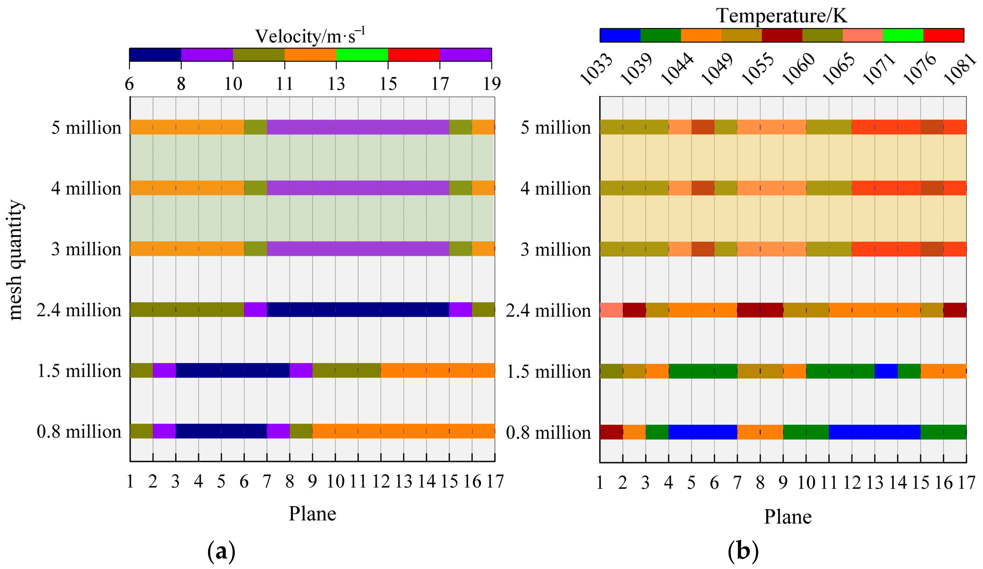
3.4. Grid Independence Verification of the Computational Model

In order to obtain the distribution of calculation and measurement parameters throughout the entire furnace, a series of cross-sections of the furnace is established as shown in Figure 4. The center of the chimney inlet is taken as the coordinate origin, and the cross-section of the furnace is taken every 0.1 m from plane 1 (Z coordinate is +1.83 m). The longitudinal Z coordinate of plane 17 is 0.23 m. Some planes are not shown in the figure, and planes 1–8 are located at the position of the cylindrical burner, where mixed gas is sprayed, and the cross-section shape are rings. Afterwards, the cross-sections (as shown in planes 9–17) are circular.

The calculation result is related to the grid generation, and the number of grids determines the calculation time, so the balance between the calculation time and the calculation accuracy should be considered comprehensively. In order to verify the mesh independence of the CFD calculation results, 17 planes were taken along the central axis of the burner at a spacing of 0.1 m (as shown in Figure 4), and the number of calculated grids was taken for a total of six working conditions ranging from 800,000 to 5 million. As shown in Figure 5, when the number of grids exceeds 3.2 million, the average speed and average temperature of each plane is compared and neither the average speed nor the average temperature of each plane changes. As shown in Figure 5a, when the number of grids exceeds 3 million, the average velocity of the 17 sections does not change with the number of grids, and the airflow velocity in the furnace decreases at the outlet of the furnace. As shown in Figure 5b, with the increase in the number of grids, the average temperature of the 17 sections fluctuates greatly. The maximum temperature level of the section is about 1060 K when the number of grids is 800,000; when the number of grids is between 800,000 and 2.4 million, the velocity field fluctuates slightly, while the temperature field fluctuates more. When the number of grids exceeds 3 million, the average speed and average temperature of each section in the furnace are stable at the same level. Therefore, 3,204,561 grid cells are used in this numerical calculation, which ensures the calculation accuracy and minimizes the calculation amount.

4. Results and Discussion

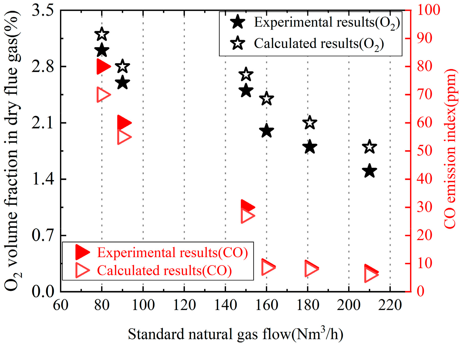
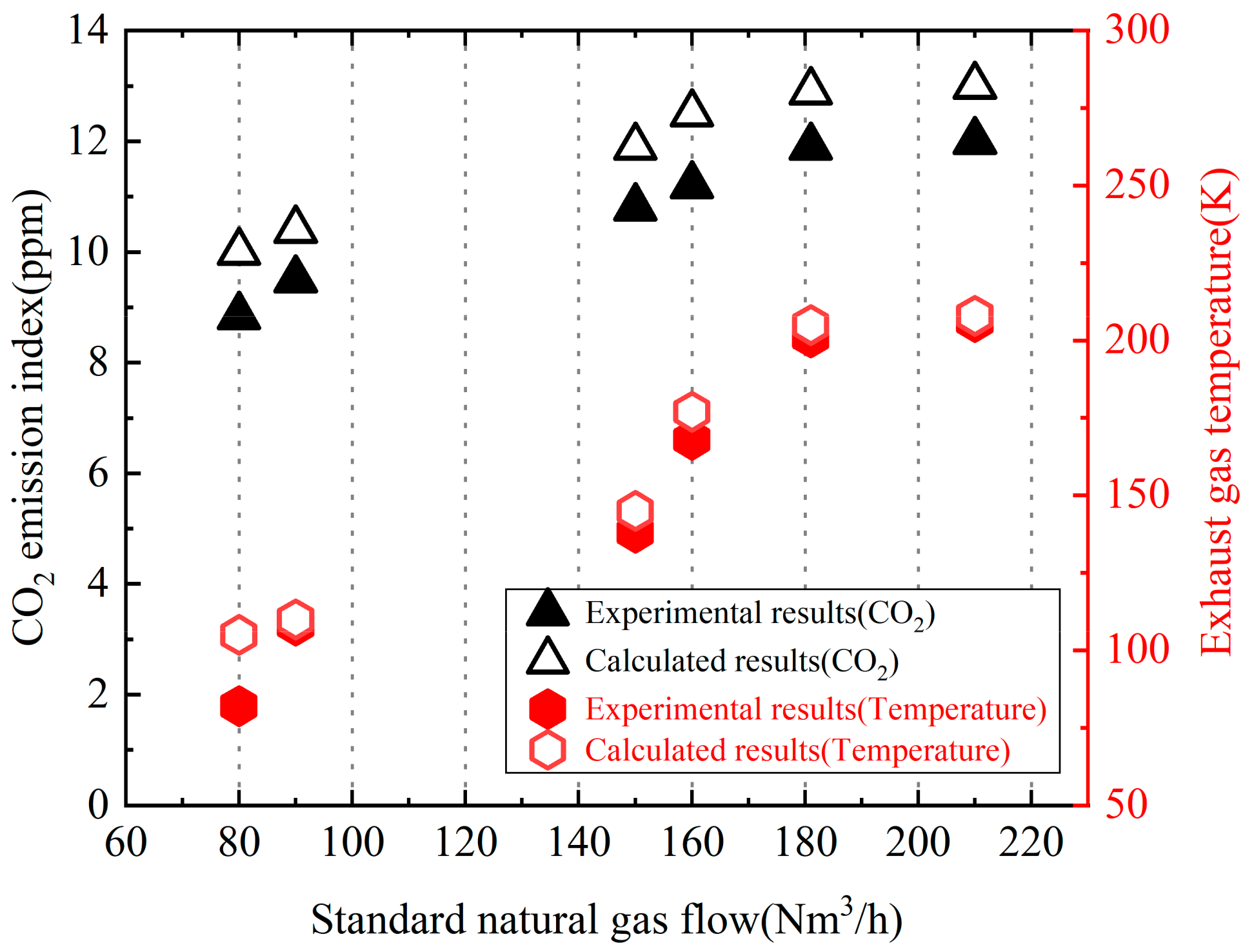
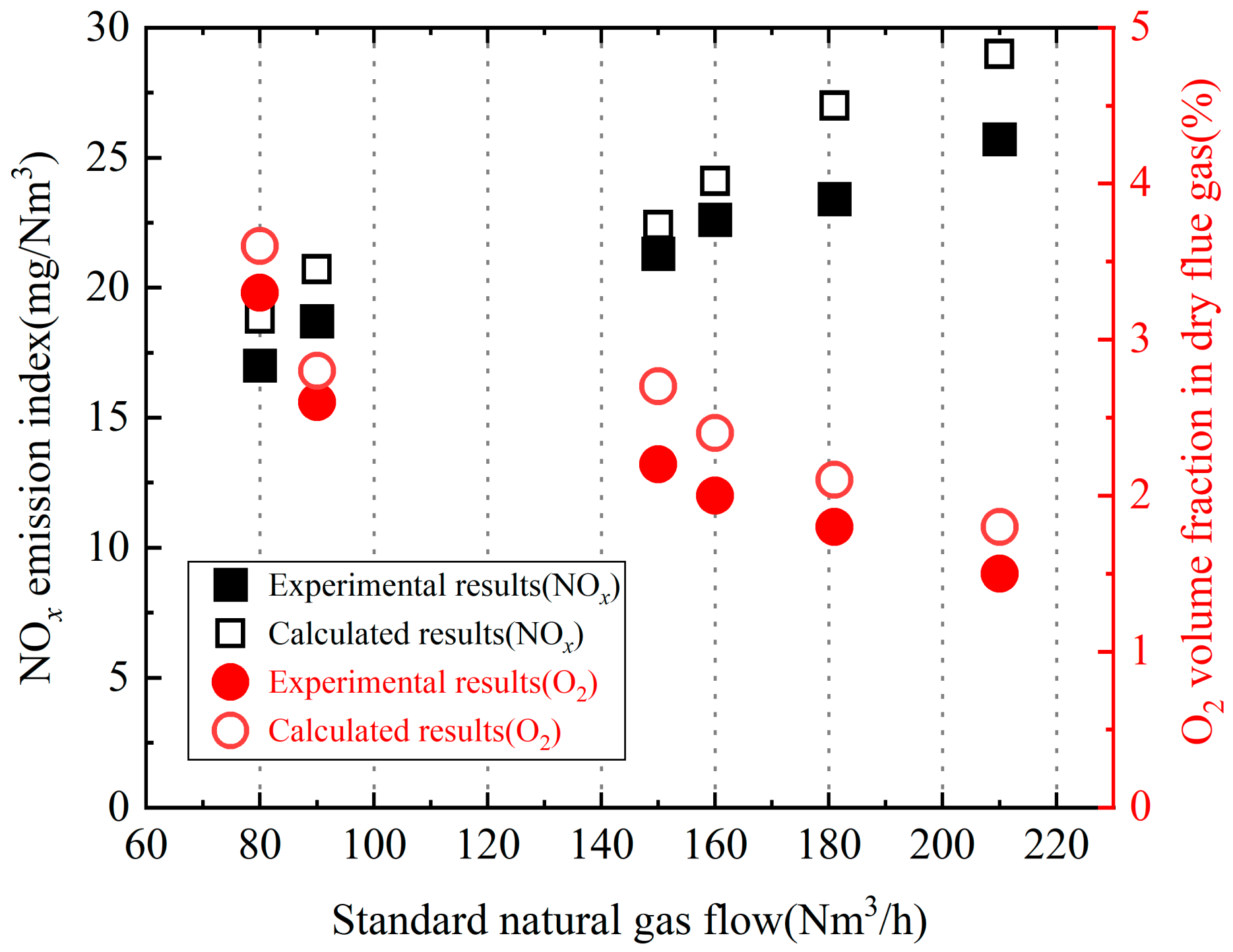
4.1. Comparison between Calculated Values and Experimental Results

The numerical calculation results are shown in Table 2, and the comparison results are shown in Figure 6, Figure 7 and Figure 8. From Figure 6, it can be seen that as the natural gas flow rate increases, the amount of O₂ gradually decreases, indicating that as the flow rate increases, the proportion of oxygen consumption increases, leading to a gradual decrease in the oxygen content in the flue gas. Moreover, as the gas flow rate increases, combustion becomes more and more complete and the CO content in the flue gas gradually decreases, indicating that the incomplete combustion component in the flue gas decreases, and more and more O₂ is consumed. When the gas flow rate is small, such as 80 Nm³/h, the CO emission reaches 80 ppm. When the natural gas flow rate is 90 Nm³/h, the actual measured CO value reaches 60 ppm. When the flow rate is 150 Nm³/h, the measured CO value decreases significantly, with a measured value of 30 ppm. This indicates that the boiler is at normal combustion conditions, and the maximum error between the measured CO value and the calculated value is 14.3%. When the gas flow exceeds 150 Nm³/h, the boiler enters a full combustion case. The minimum measured CO flow rate of the boiler is 7 ppm and the O₂ content in the flue gas is 1.5, indicating that most of the O₂ content in the flue gas is consumed by the natural gas. The maximum error between the measured and calculated O₂ content is 16.7%. The measured value of CO is greater than the calculated value, which is because although the calculated working condition is a non-adiabatic wall, radiation heat transfer is not included, so the calculated temperature is higher than the measured temperature. A high-temperature environment is conducive to complete combustion of CO. The amount of O₂ in the flue gas shows the same trend as the content of CO; that is, a low amount of O₂ indicates sufficient combustion, an increase in O₂ consumption, an increase in CO reaction of intermediate combustible materials, and a decrease in CO content in the flue gas.

The exhaust temperature and CO₂ emissions of boilers are important indicators for measuring boiler economy, and the exhaust temperature should be within a reasonable range to ensure boiler economy. As shown in Figure 7, the comparison between the calculated and measured values of boiler exhaust temperature and CO₂ emissions are compared. As can be seen from the figure, as the amount of gas increases, the exhaust temperature of the boiler increases rapidly. This is because a large amount of gas is burned and releases a large amount of heat, and the heat absorption of the boiler wall’s water-heating surface is not as fast as the heat release of the gas, resulting in an increase in exhaust temperature. The maximum exhaust temperature is 202 °C, and the calculated exhaust temperature is higher than the measured value, which is consistent with the theory in Figure 6. The calculated temperature is slightly higher than the measured temperature, causing the calculated exhaust temperature to be slightly higher than the measured exhaust temperature. The maximum error between the two is 28%, which occurs when the flow rate is the lowest; that is, when the natural gas flow rate is 80 Nm³/h, the combustion condition is unstable at this time and the fuel incomplete combustion loss is significant. When the gas flow rate is 80 Nm³/h, the CO emissions are the highest among the six operating conditions and the maximum calculation error is 5.1% among the other five operating conditions. The calculated values are in good agreement with the measured values. As the fuel consumption increases, the CO₂ emissions gradually increase, but the increase is not significant. The maximum error between the calculated and measured CO₂ values occurs at the lowest flow rate, with a maximum error of 13.1%. The calculated and measured values are in good agreement. The calculated values of exhaust gas temperature and CO₂ value are higher than the measured values due to the semi-adiabatic working condition (ignoring radiation heat transfer), which leads to an increase in temperature and CO₂ displacement due to sufficient combustion.

The denitrification effect is an important indicator of boiler emissions, and the emission of NO_x is currently an important monitoring value for clean combustion. Under different gas flow conditions, the measured and calculated values of O₂ and NO_x emissions in flue gas are compared, as shown in Figure 8. In the figure, it can be seen that except for the minimum flow rate (i.e., when the gas flow rate is 80 Nm³/h), the NO_x emissions show an increasing trend with the increase in flow rate. This is because thermal NO_x dominates, accounting for 31.1% of the total NO_x [52]. As the flow rate increases and the exhaust temperature increases (as shown in Figure 7), the generated thermal NO_x shows an increasing trend. At the same time, due to the increase in flue gas volume, the total NO_x emissions increase. The calculated NO_x generation value is higher than the actual measurement value, which is caused by the high temperature in the calculated furnace. This is consistent with the previous conclusion, with a maximum calculation error of 15.4%. Under six operating conditions, the NO_x emission value is lower than 30 mg/Nm³ and the emission standard meets the environmental protection requirements of Beijing-Tianjin-Hebei.

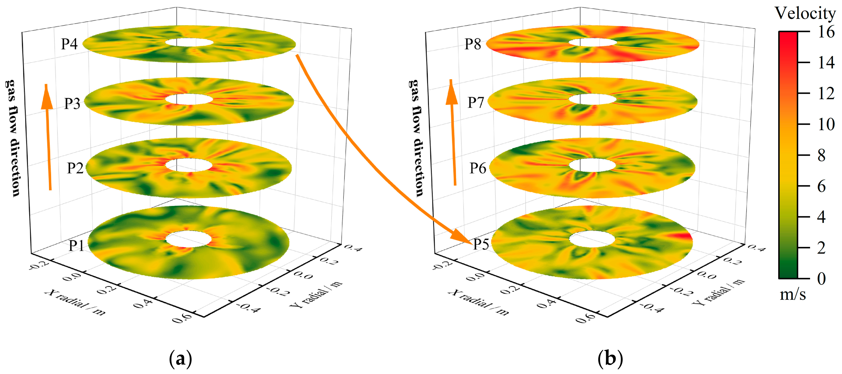
4.2. Distribution of Gas Flow Field inside the Furnace

The different pore structures of surface burners have varying degrees of impact on combustion conditions and pollutant emissions. Jorn Hinrichs et al. [20] and Rachel Lamioni et al. [52] used a circular hole and rectangular strip structure surface burner. Jorn Hinrichs et al. [20] concluded that hydrogenation conditions can lead to a varying degree of decrease in NO. Through research, Rachel Lamioni et al. [48] also found that the NO content at the flame front position suddenly increases, although the NO production also increases afterwards. However, the growth rate is much smaller than the flame front position, and in order to comprehensively consider the production of nitrogen oxides, the generation of NO₂ should also be considered.

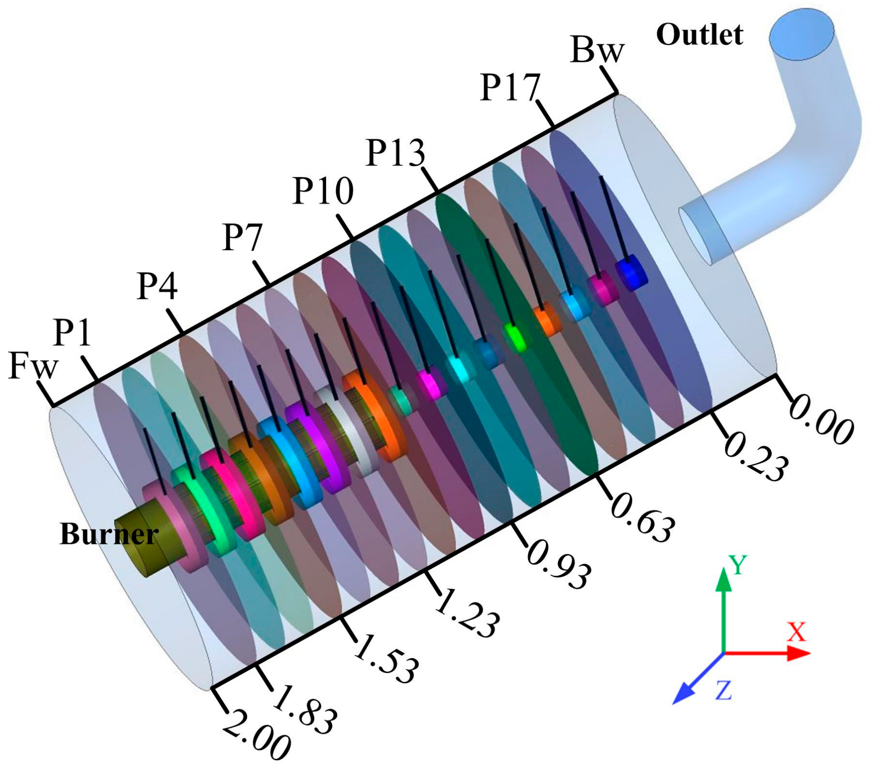
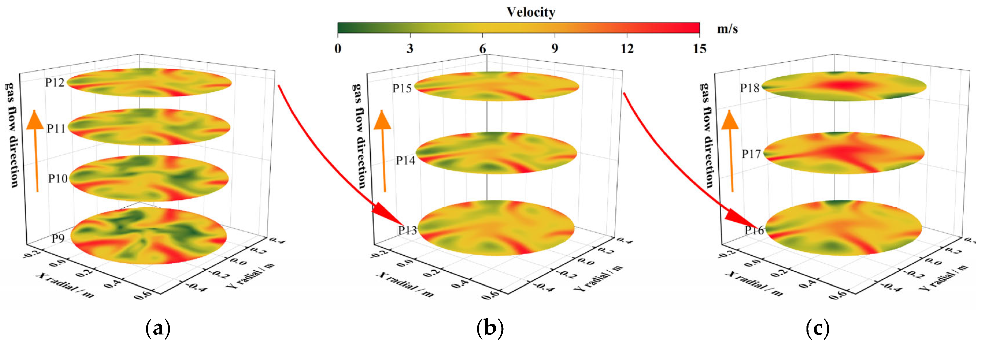
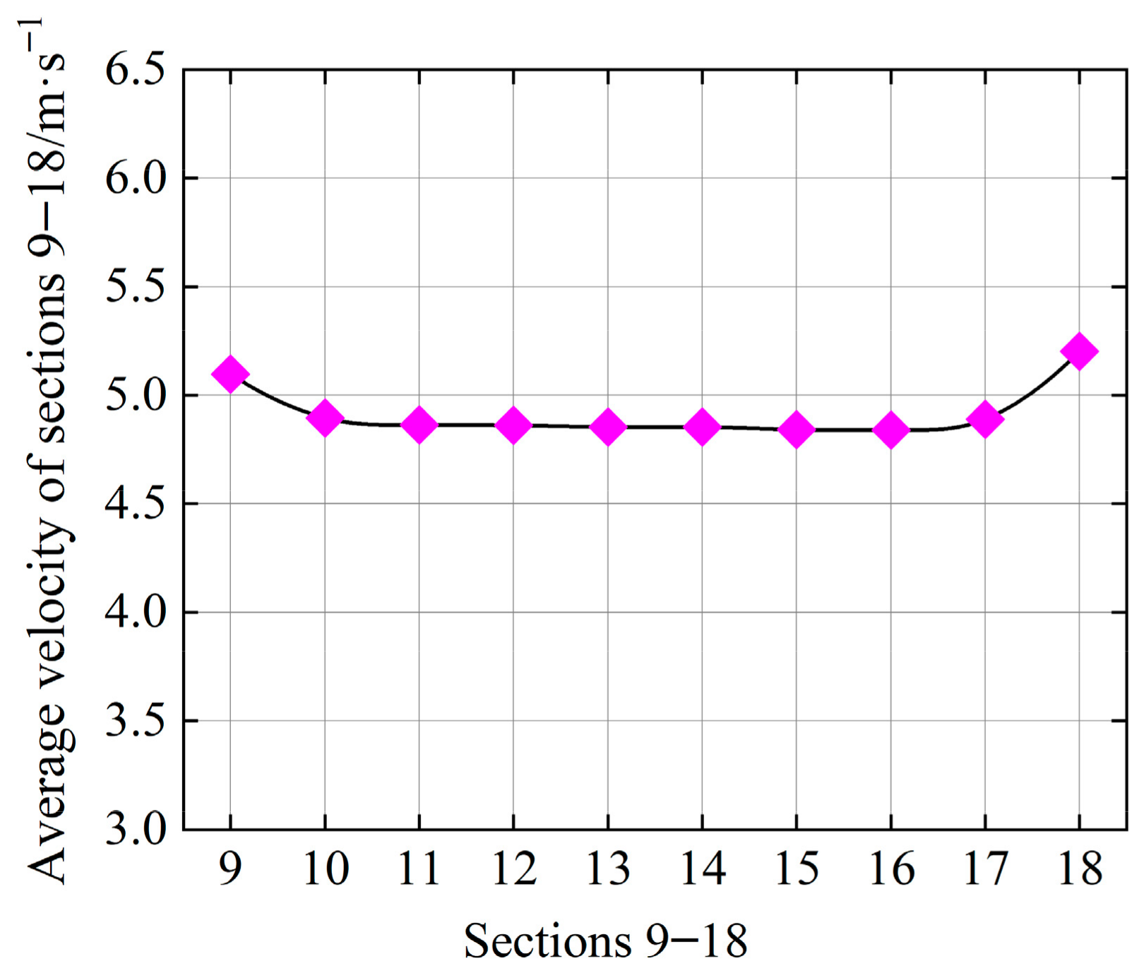
Distribution of Velocity Fields in Different Planes in the Furnace

The flow field inside the furnace has a significant impact on combustion and boiler emissions, especially on the temperature distribution inside the furnace, which is an important basis for emissions and other indicators. Therefore, analyzing the distribution characteristics of the flow in the furnace is of great significance. As shown in Figure 4, the velocity cloud maps are created on section P1–8 of the burner area based on the calculated data to analyze the flow field inside the furnace. Due to the cylindrical structure of the fully premixed burner, the cross-section smoke flow direction cloud diagram shows a “fan blade” shape.

As shown in Figure 9a, the airflow has just entered the burner; that is, at the inlet of the burner. Due to the high resistance of the surface opening at this point, most of the airflow flows towards the rear of the burner (see section P1 cloud diagram). As the airflow flows towards the rear of the burner to P2, the velocity of the airflow entering the furnace from the square hole significantly increases and it is symmetrically distributed around the combustion tube. The airflow shows an attenuation trend after flowing out of the combustion hole. The airflow velocity at plane P3 slightly increases compared to P2. At position P4, the airflow velocity slightly decreases because there is a single hole relative to P4 and the airflow velocity increases along the airflow direction to P5, as shown in Figure 9b. The airflow cloud diagram is similar to P3 as P5 and P3 are symmetrical structures relative to P4, and the average velocity of the P5 plane is higher than the average velocity of plane P3. This is because the upward pressure of the airflow direction gradually increases, leading to an increase in the flow rate of the nozzle, and the speed gradually increases from the head to the tail of the burner. Due to the highest pressure located at the rear of the burner, the P8 plane has the highest velocity relative to the front planes (P1–P7) on the entire plane. The velocity distribution of the combustion cylinder has the following characteristics: low in the front and high in the rear, with plane P3 and plane P5 symmetrically distributed on both sides of plane P4. This characteristic can be seen more clearly from Figure 10. Figure 10 shows the average velocity on planes P1–P8.

Due to the limitations of cloud image reaction speed, taking the average of each plane velocity reflects the changes in the entire plane velocity distribution relative to other plane velocities, thus enabling a more accurate understanding of the velocity field in the furnace. From Figure 10, it can be seen that there is a low valley in the velocity of each plane to P4. This is because the opening here is a single square hole, while the other positions are rectangular grooves, where the airflow resistance is the highest, resulting in a decrease in flow velocity. The velocity levels of plane P3 and plane P5 exhibit symmetry on both sides of P4, while the average velocity of P5 is slightly higher, which is consistent with the conclusion drawn in Figure 9. The average velocity of section P6–8 gradually increases until P8 reaches the maximum value among the eight planes, and the same conclusion as Figure 9 is drawn. Figure 9 and Figure 10 show a gradual increase in the average velocity of the cross-section, except for P4, as it penetrates deeper into the furnace. Specifically, for each cross-section, the airflow velocity distribution along the circumferential direction of the cylindrical burner is uniform and the gas velocity gradually decreases towards the wall direction.

As shown in Figure 11, the velocity distribution of each section is relatively uniform along the direction of flue gas flow to the tail of the boiler. Specifically, for the area with higher plane velocity on planes P9–12, it is distributed near the furnace wall. As the airflow moves towards the tail, the airflow distribution gradually becomes uniform. Overall, the airflow exhibits symmetry around the entire cross-section, and the high-speed airflow area can be evenly distributed around the furnace.

Specifically, from Figure 11, planes P9–12 show a low speed zone of 6 m/s and a high speed of 10 m/s. The difference between the maximum and minimum values of plane velocity in P9 is significant, and the plane velocity in P12 gradually tends to be uniform. As the airflow flows towards the rear of the boiler, on planes P13–15 the velocity tends to be more uniform. The high-speed area of planes P16–18 moves towards the center of the section, and the high-speed area of plane P18 is concentrated in the center of the plane, indicating that the airflow has already converged towards the center and entered the chimney inlet. The distribution of airflow velocity on planes P13–18 is relatively uniform, with little difference in velocity across the entire plane. Taking P17 as an example, the maximum velocity value is 9 m/s and the minimum velocity value is 7 m/s. Figure 12 shows the average velocity values on a total of ten planes, P9–18.

From Figure 12, it can be seen that there are a total of ten planes on planes P9–18, of which pane P9 and plane P18 have higher velocities. This is because plane P9 is located at the tail of the cylindrical burner, where a large amount of mixed gas still flows out, resulting in a higher airflow velocity. For plane P18, the gas converges at the chimney inlet, resulting in a higher average airflow velocity throughout the plane. For plane P10–17, the average velocity of each plane is around 4.7 m/s and the airflow distribution is relatively uniform. Therefore, from the velocity cloud in Figure 11 and the average velocity curve in Figure 10 and Figure 12, it can be seen that the airflow velocity distribution outside the combustion tube is relatively uniform and there is no velocity vortex zone or velocity “dead lag” zone in the entire velocity plane. The uniformity of velocity characterizes the uniform mixing of fuel, and the uniformity of airflow and velocity throughout the furnace is the foundation for subsequent full combustion and clean combustion.

4.3. Temperature Field Distribution in Furnace

The temperature field inside the furnace is based on the uniformity of the airflow inside the furnace, and the distribution and uniformity of the temperature field inside the gas boiler furnace have a significant impact on the generation of pollutants. Therefore, it is necessary to analyze the temperature field inside the furnace.

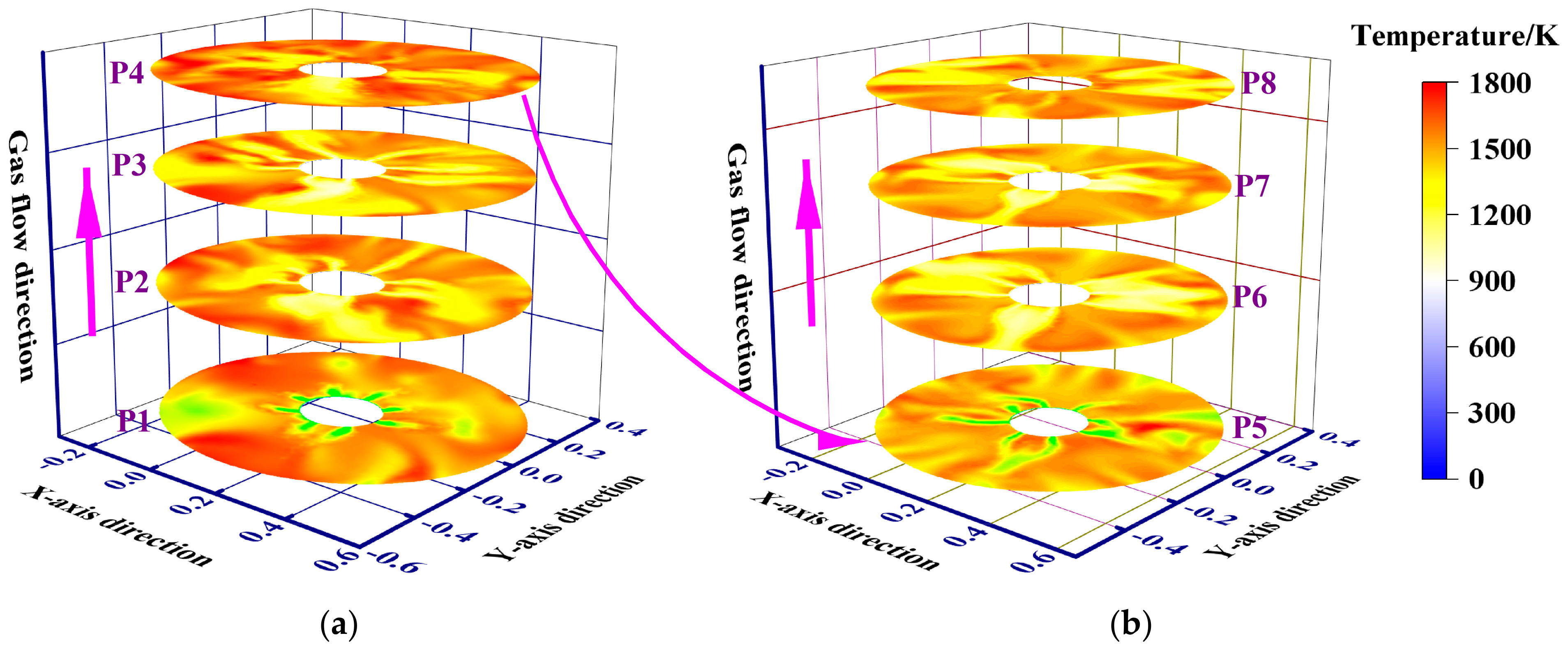
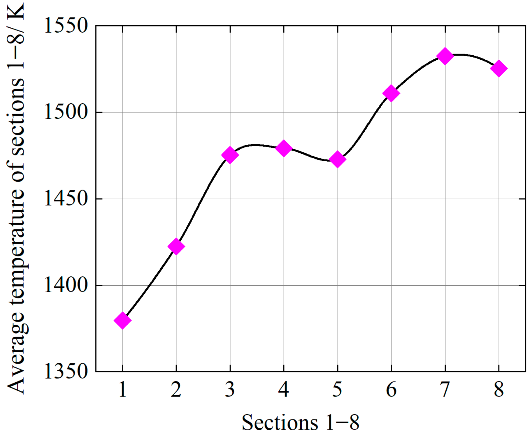
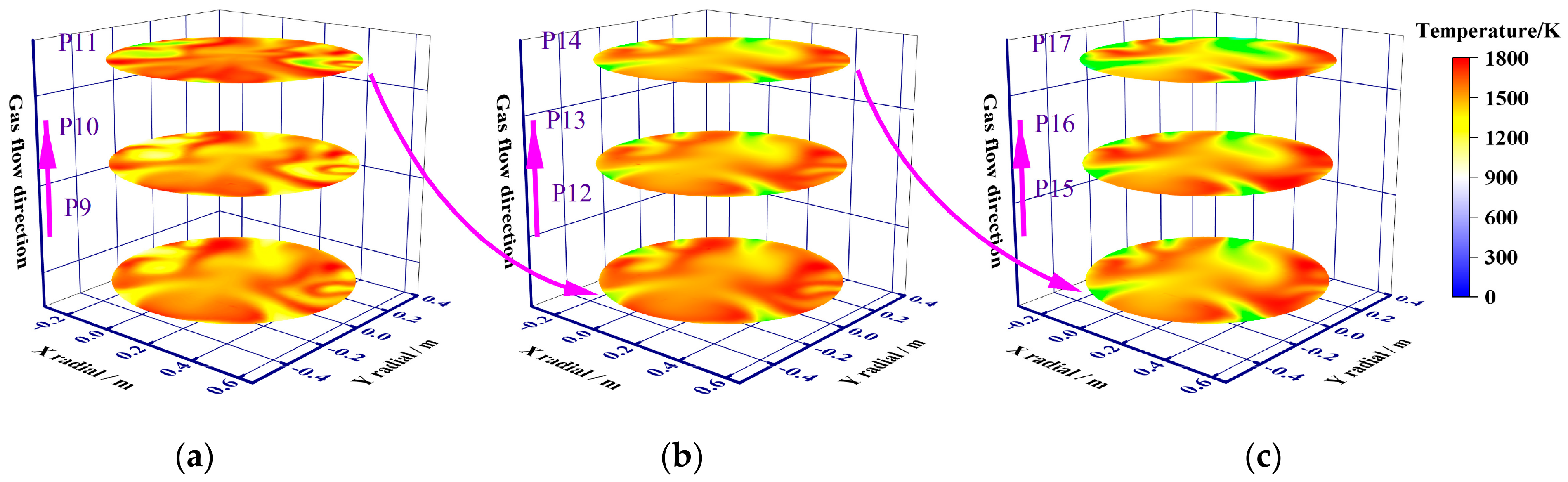
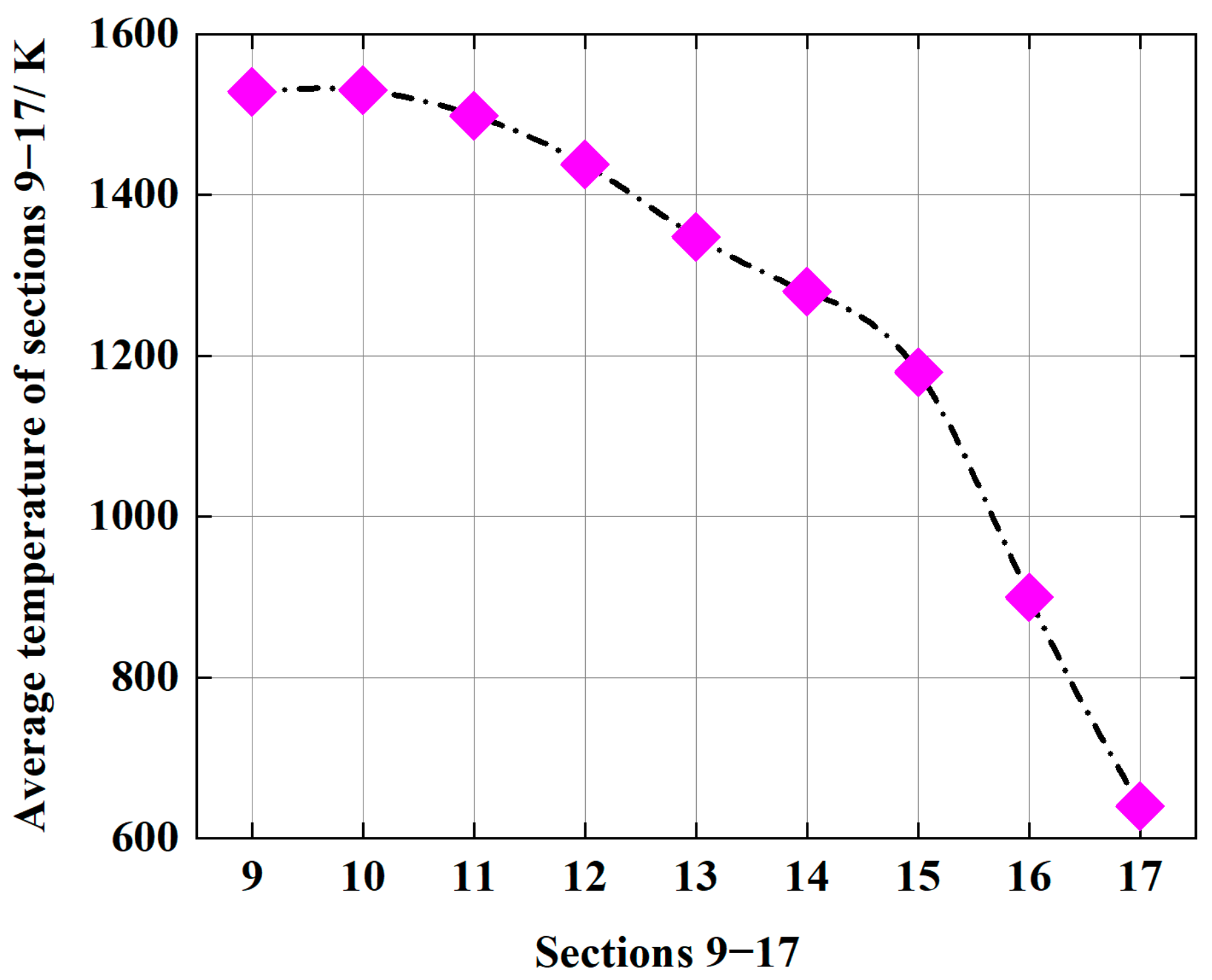
4.3.1. Temperature Field on the Planes in the Furnace

The temperature field distribution inside the furnace is studied using the cross-sectional location diagram in Figure 4, which refers to the position from the cylindrical burner to the plane of the boiler flue gas outlet. The position z = 0 is the rear furnace wall of the boiler, as shown in plane 18 in the figure.

As mentioned earlier, the distribution of gas flow field in the furnace is relatively uniform and the combustibles in the furnace are well filled. As shown in Figure 13, on Section 1–8 of the burner area, a temperature cloud map is created based on the calculated data to analyze the temperature field inside the furnace. From Figure 13, it can be seen that it is located near the front wall of the combustion tube. Due to the relatively close proximity to the front wall, the mixed gas flows into the furnace as soon as it enters the burner. The amount of mixed gas here is relatively small and close to the front wall of the boiler. Therefore, the combustion temperature here is relatively low and there is a spoke-shaped low-temperature zone at the gas outlet (as shown in Figure 13, plane P1). As the gas flows towards the depth of the combustion tube, the amount of gas increases and the high-temperature area gradually expands due to the thermal radiation inside the furnace (as shown in Figure 13, plane P2). There is a slight change in the high-temperature areas of planes P3 and P4, but the change is not significant. The high-temperature area of plane P4 is the largest among the four planes.

At plane 5, a spoke-shaped low-temperature zone appears again in the temperature area because the nozzle is located at the second strip nozzle and there is no mixed gas spraying at the top of the strip nozzle, resulting in a local temperature decrease. However, the overall temperature level of the cross-section is higher than that of plane P1. As the airflow flows towards the rear of the combustion tube, the high-temperature area in plane P6 further expands, with a slight increase in temperature compared to the previous planes (P1, P2, P3, P4, P5). The high-temperature area in plane P7 expands to its maximum, and the temperature development trend in the combustion tube area can be seen more clearly from the comparison of the average temperature of each plane in the combustion tube area, as shown in Figure 14. As shown in Figure 14, the minimum temperature on planes 1–8 is 1106.7 °C (on plane P1) and the maximum temperature on plane P7 is 1232.4 °C. Specifically, since plane P1 is located in the front of the combustion cylinder, less combustible gas enters the furnace and, thus, the combustion temperature is relatively low. With the continuous flow of combustible air into the furnace, the average temperature of section P4 gradually increases. The temperature rise of section P4 is smaller than that of section P3 because there is no air inlet at the back of section P4, resulting in a smaller gas flow in this section. As a result, the combustion temperature of the whole section does not increase much compared with that of section P3. Due to the lack of gas openings in the front of section P5, the average temperature of the section relative to P4 is slightly decreased. The average temperature is gradually increased on subsequent sections P6/P7, and the temperature of section P8 is slightly decreased compared to P7, but the decrease is not significant. This is because P8 is located at the tail of the combustion tube and the gas flow rate is relatively reduced. However, due to its location in the middle of the furnace, both front and back are in the combustion vigorous zone so the temperature changes relatively little compared to P7.

The above analysis shows that the combustion chamber area belongs to the area where the airflow is concentrated and flows out, and the airflow disturbance is relatively strong. When the flue gas flows to the area outside the combustion tube, the temperature cloud maps of each plane are shown in Figure 15. As shown in the Figure, the high-temperature area of plane P9 in the rear furnace area of the combustion tube has significantly expanded, indicating that the combustible gas continues to burn here, leading to the expansion of the average temperature and high-temperature area of the cross-section. The high-temperature area on plane P10 reaches its maximum and the average temperature of this section also reaches its maximum. A significant low-temperature area appears on plane P11, indicating that the combustion intensity here has begun to weaken and has exceeded the position of the front. As shown in Figure 15b, there is a clear low-temperature area in this group of planes, and the low-temperature area gradually expands, further indicating that it has exceeded the combustion front and the combustion temperature shows a downward trend. As shown in Figure 15c, the low-temperature region further expands, indicating a decrease in combustion intensity, leading to a decrease in combustion temperature and a decreasing trend in the entire cross-section temperature. The average temperature of plane P17’s section is 336.7 °C, and the highest temperature of this section is 424.8 °C. From P1–P17, it can be seen that after the mixed gas flows out of the burner, the temperature inside the furnace reaches the highest value between plane P9 and plane P10, indicating that this is the center of furnace combustion. Afterwards, as the flue gas flows towards the chimney, the low-temperature area gradually expands and the low-temperature area on plane P17 expands to the maximum area in the described plane. As can be seen from the figure (P11 in Figure 15a), the low-temperature zone of the plane extends from the inner wall of the furnace to the center and the non-adiabatic wall is set in the calculation, indicating that heat is transferred to the medium inside the furnace at the furnace wall. At plane P17, due to the combined effect of the decrease in combustion temperature and heat transfer at this point, the temperature of this section decreases to the lowest.

In order to more accurately analyze the temperature distribution characteristics on planes P9–P17, the average temperature values on each cross-section were taken for comparison, as shown in Figure 16. From the figure, it can be seen that the average temperature on planes P9, P10, and P11 continues to increase compared to the average temperature on P8. Specifically, the average temperature of plane P10 reaches the maximum value of 1257.7 °C and the temperature levels on sections P9 and P12 are equivalent, which is slightly lower than section P10 at 1255 and 1227 °C. From this, it can be seen that the position of the combustion center in the furnace is near section P10. Afterwards, the average temperature of each section gradually decreased until the average temperature on section P17 dropped to 336.7 °C. On section P9–P13, the temperature decrease is relatively slow, exceeding that of section P13 (P14–P17), and the temperature decrease is relatively rapid, indicating a decrease in combustion intensity in the furnace. It also proves that the flame length of the natural gas combustible mixture’s combustion is short and the temperature distribution in the furnace is relatively uniform. The temperature drops to 180 °C at the outlet of the furnace.

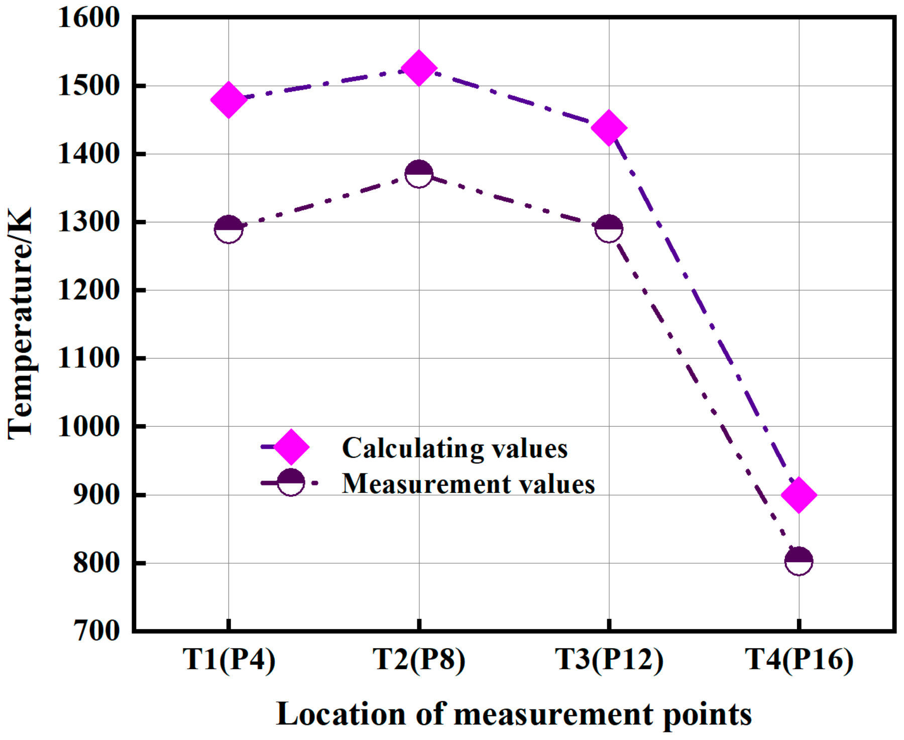
4.3.2. Comparison of Measured Temperature and Calculated Value in Furnace

Based on a comprehensive analysis of planes P1–P17 (Figure 13, Figure 14 and Figure 15), the temperature at the front wall of the furnace is relatively low at 1106.7 °C. Although some low-temperature areas are shown in the cloud image at section P5, the average temperature of the entire section is still in an upward stage. At section P10, the temperature reaches its maximum value. As the combustion intensity weakens, the average temperature on the section after P10 gradually decreases, and at P17, the temperature drops to 336.7 °C. And, each section gradually expands from the low-temperature area at P11. This is because the boiler wall is set as a non-adiabatic wall and heat is transferred from the flue gas to the medium inside the furnace, resulting in a decrease in temperature at the furnace wall. As the flue gas flows towards the tail of the boiler, the expansion trend of the low-temperature area accelerates, and the average temperature of the section decreases.

In order to verify the accuracy of numerical calculations, temperature measurement hot sockets are arranged at the corresponding positions on the furnace outer wall. The four thermocouple measurement points, T1, T2, T3, and T4, correspond to sections P4, P8, P12, and P16 in sequence. The specific positions of temperature measurement thermocouple openings are shown in Figure 1a. The plug-in temperature thermocouple is shown in Figure 17, with a maximum measurement temperature of 2030 °C and a measurement accuracy of Class I. The plug-in temperature thermocouple shown in Figure 17 has a temperature sensor wire that can be cut based on the temperature measurement position and the sensor wire can be replaced. Therefore, its temperature measurement accuracy is greatly improved compared to infrared thermocouples.

The temperature thermocouple shown in Figure 17 is used to measure the temperature at the insertion hole position mentioned above and four positions in the diameter direction at the same temperature measurement hole are selected for temperature measurement. The average measurement value is taken and compared with the calculated value. The comparison between the measured temperature and the average calculated temperature of each section is shown in Figure 18.

As shown in Figure 18, the actual measurement value is lower than the calculated value, and the maximum error between the two occurs at measurement point T1 (P4), with a maximum error of 13.7%. As the flue gas flows towards the axial depth of the boiler, the error between the two gradually decreases, with an error of 10% at measurement point T2 and 8.8% at measurement point T3. Overall, the error between the calculated and measured values is less than 15%. At measuring point T1, it is located on the outer side of the combustion tube, where the airflow disturbance is relatively strong. Therefore, the temperature measurement error is relatively large. At measuring point T2, which is located at the tail of the combustion tube, the airflow disturbance is relatively weakened and the measurement error is reduced to 5.9% at measuring point T4. The calculated values are in good agreement with the measured values as a whole.

4.3.3. Summary of Temperature Field Distribution in the Furnace

As described in Section 4.3.1 and Section 4.3.2, the overall temperature field in the furnace shows a trend of first increasing and then decreasing from front to rear. The highest temperature at a single point appears near plane 10, and the lowest temperature in the entire furnace is at the furnace outlet. Due to the uniform distribution of air flow in the furnace, which lays the foundation for good combustion in the furnace, the temperature field distribution in the furnace is relatively uniform. Moreover, the trend of temperature field changes is relatively gentle, and the high-temperature and low-temperature regions are excessively smooth. The temperature field in the radial direction of the furnace also shows a trend of first increasing and then decreasing. This is because the wall is set as a non-adiabatic wall during the calculation process and there is continuous heat transfer to the heating surface—the water-cooled wall. Overall, the trend of the calculated temperature inside the furnace is similar to the actual operating trend. The maximum error between the experimental and calculated values is 13.7%.

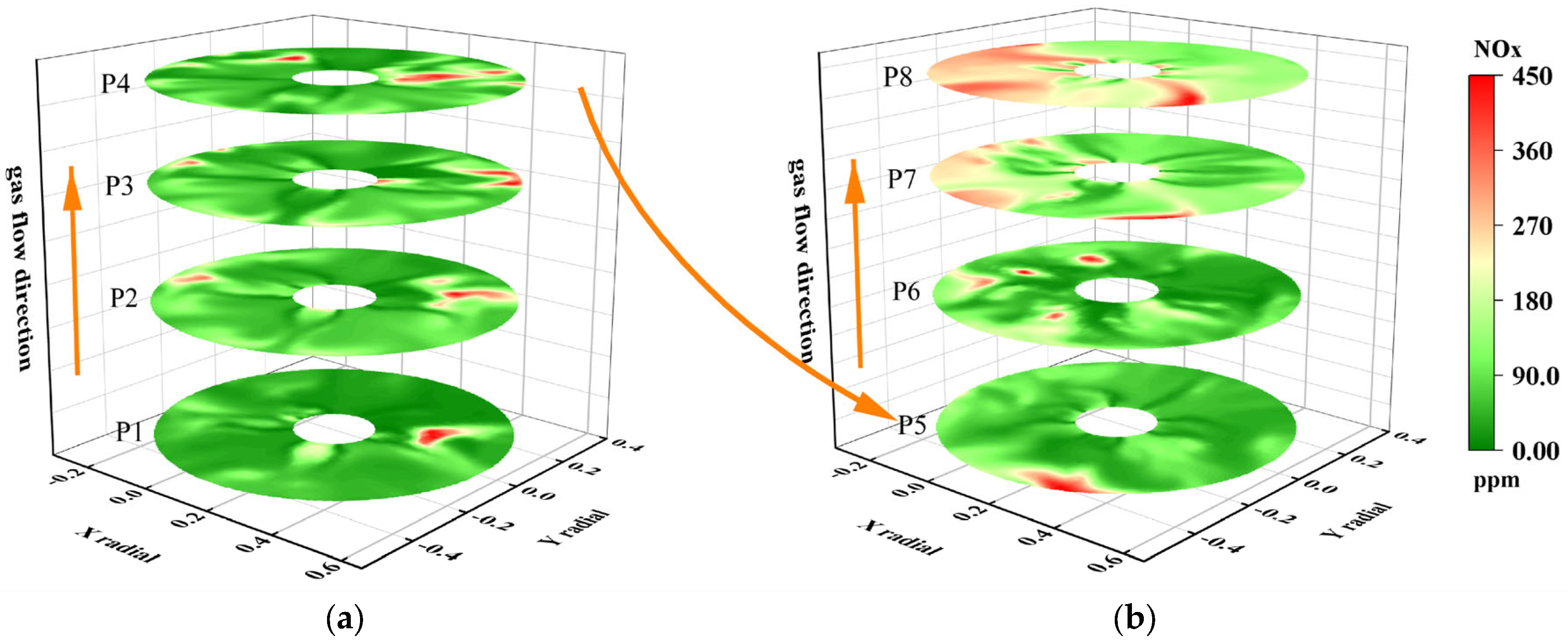
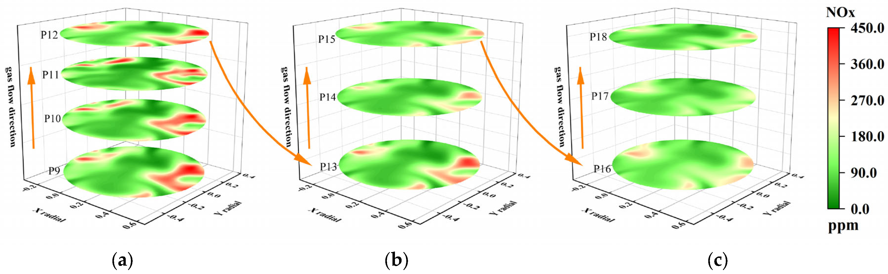
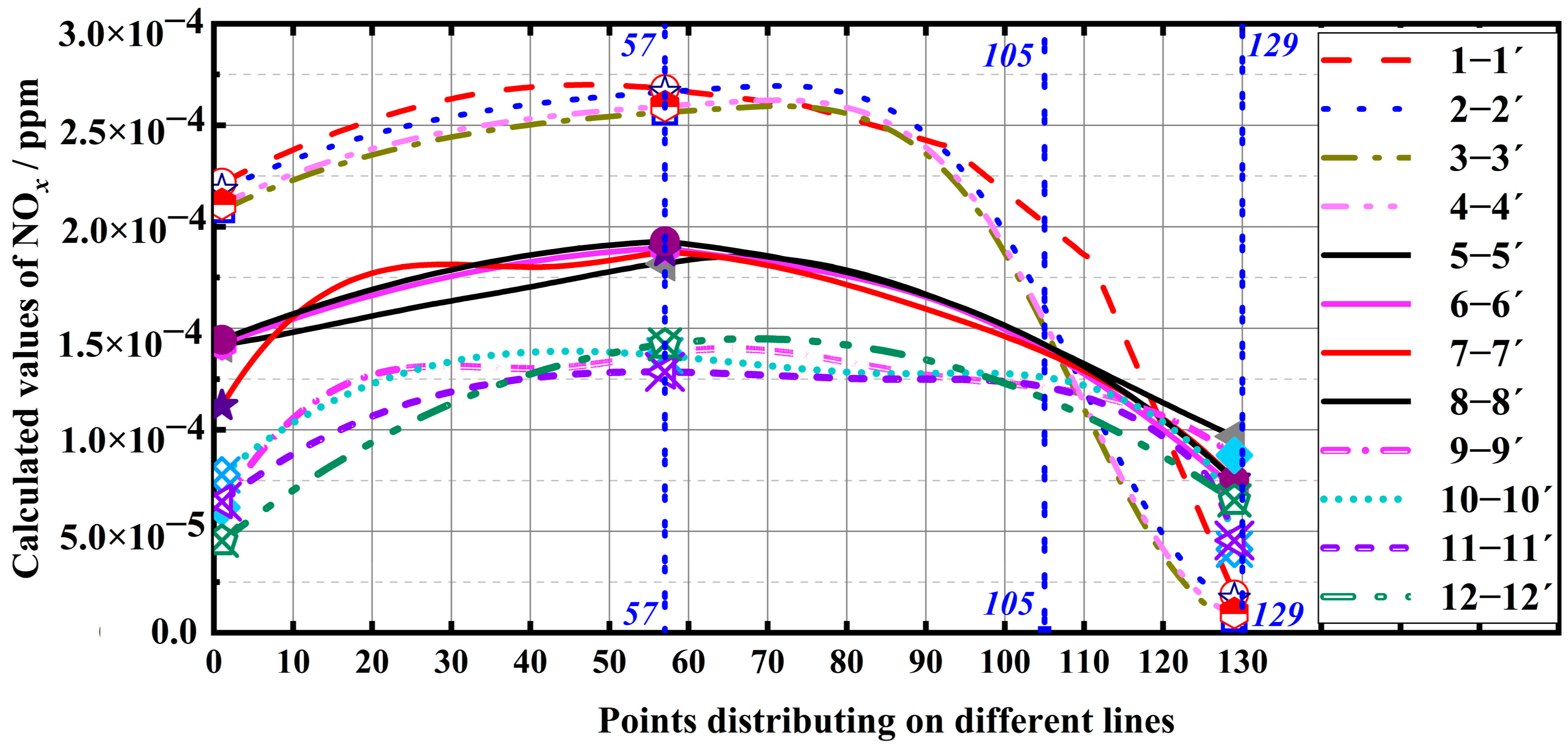
4.4. Analysis of NO_x Calculated Values

NO_x emission is a key monitoring object for boiler pollutant emissions. In order to comprehensively measure the generation and emission status of NO_x, a cloud map distribution of NO_x generation is still made on the cross-section shown in Figure 4 to evaluate the NO_x generation status in the furnace. As shown in Figure 19, the NO_x distribution cloud maps were drawn on planes P1–P8, as described in Figure 4.

From Figure 19, it can be seen that the amount of NO_x generated on the plane located in the burner area gradually increases along the airflow direction. Specifically, as shown in Figure 19a, at the front wall of the boiler just as the gas enters the burner, combustion enters the initial stage, as described in Section 4.3.1. Due to the temperature-type NO_x being the main NO_x in the furnace, the NO_x generated on plane P1 is below 100 ppm, with only one point generating 400 ppm of NO_x. As the airflow flows deeper into the boiler, the amount of NO_x generated on plane P4 does not change much compared to plane P1. The number of points with higher NO_x generation slightly increases compared to plane P1, but the NO_x content in most areas on the plane is below 100 ppm. Planes P1–P4 belong to the low-NO_x production area. As shown in Figure 19b, the trend of NO_x generation gradually increasing along the airflow direction is more obvious when entering the second half of the burner. Specifically, the NO_x generation in local areas on plane P5 reaches over 420 ppm. As the airflow flows deeper, there are more than four points exceeding 200 ppm on plane P6, and the 100–200 ppm content area is significantly expanded relative to P5. On plane P7, several areas exceeding 300 ppm have been connected into sheet-like areas, accounting for more than 1/4 of the plane area. On plane P8, the high-NO_x-content area continues to expand, with areas exceeding 300 ppm accounting for more than one-third of the plane area. Overall, the NO_x content on plane P1-P4 shows an increasing trend, but the increase is not significant. In the second half of the burner, NO_x still shows an increasing trend on planes P5 and P6, but the average NO_x ppm value is still below 180 ppm. The NO_x ppm value increases rapidly on planes P7 and P8, with an average ppm value of 240 ppm on plane P7 and 320 ppm on plane P8.

The NO_x distribution cloud map outside the burner, also known as planes P9–P17, is shown in Figure 20.

As shown in Figure 20, on the planes P9–P12 outside the combustion chamber, the NO_x content gradually decreases along the airflow direction, but the decrease is not significant. The highest NO_x value on the four planes reaches 300 ppm. On planes P9–P11, there is a significant amount of NO_x production, with a converted NO_x volume content of 162 mg/m³. The airflow continues to flow towards the tail of the boiler, reaching the P13–P15 planes. Compared to the P9–P12 planes, the NO_x generation is significantly reduced. The main reason is that the flame front is located near P10, and the position of P13–P15 is far from the flame front. The temperature on the entire plane decreases, resulting in a smaller temperature-type NO_x production. The highest NO_x value on plane P13 is 280 ppm, and the highest value on plane P14 is 260 ppm. On plane P15, the NO_x value decreases to 231 ppm. The airflow continues to flow towards the tail of the boiler, reaching the P13–P15 planes. Compared to the P9–P12 planes, the NO_x generation is significantly reduced. The main reason is that the flame front is located near P10, which is far from the flame front position. The temperature on the entire plane decreases, resulting in a smaller temperature-type NO_x production. The highest NO_x value on plane P13 is 280 ppm, and the highest value on plane P14 is 260 ppm. The value on plane P15 decreases to 231 ppm.

In order to evaluate the production status of NO_x in various parts of the cylindrical furnace, 12 straight lines were taken in the furnace, and the relationship between each line and the plane position (as shown in Figure 4) is shown in Figure 21.

As shown in Figure 21, 12 straight lines are taken in the cylindrical furnace space according to the position in the figure. As shown in the main view of Figure 21a, four straight lines are uniformly taken on a cylindrical surface with a radius of 0.38 m: 1-1′, 2-2′, 3-3′, 4-4′; four straight lines are uniformly taken on a cylindrical surface with a radius of 0.28 m, 5-5′, 6-6′, 7-7′, 8-8′, with a spacing of 30° between the above four straight lines and the four straight lines on the cylindrical surface R = 0.38 m; on a cylindrical surface with a radius of 0.18m, four straight lines, 9-9′, 10-10′, 11-11′, 12-12′, are uniformly taken. The above four straight lines are spaced 30° apart from the four straight lines on the cylindrical surface R = 0.28 m. It can be seen that the endpoints of the 12 straight lines in the furnace are located on planes P1 and P17. Due to the fact that the four corresponding straight lines are located symmetrically along the central axis, the NO_x values at the corresponding points should theoretically be the same. Therefore, the 12 straight lines represent the generation of NO_x in most positions within the furnace.

On each straight line segment shown in Figure 21, 129 points were continuously and uniformly selected, and the calculated values of NO_x at each point were extracted. The trend of the calculated values is shown in Figure 22. From the figure, it can be seen that among the twelve three groups of straight lines, the outer four lines, 1-1′, 2-2′, 3-3′, and 4-4′, have higher calculated NO_x values than the other two groups of straight lines before point 105. The trend of NO_x generation values calculated on these four lines is consistent. Specifically, the minimum NO_x generation value at the inlet of the burner on each straight line is 200 ppm. Afterwards, the NO_x generation value gradually increases. At point (number 57), the calculated NO_x generation value reaches its maximum, and the maximum calculated NO_x on the four lines is 270 ppm. As the gas flows towards the rear of the boiler, the calculated NO_x value on the four outer straight lines gradually decreases, but the decrease amplitude increases compared to the first 57 points and reaches point 129 at the rear of the furnace. The calculated value of NO_x is the lowest among the four straight lines, which is 10 ppm. If converted into a mass volume content, the value is 20.5 mg/Nm³. For the four straight lines located in the middle of the plane, namely lines 5-5′, 6-6′, 7-7′, and 8-8′, the calculated NO_x values have decreased compared to the four outer straight lines, and the change in NO_x calculated values has slowed down. Specifically, the lowest calculated NO_x value for the four straight lines at the burner inlet, i.e., the starting point of the straight line, is 110 ppm. At point 57 of the straight line, the highest calculated NO_x value reaches 197 ppm, and then the calculated NO_x value gradually decreases, As the flue gas continues to flow towards the rear of the boiler, the minimum calculated value of NO_x at point 129 is 80 ppm. For the four innermost straight lines, 9-9′, 10-10′, 11-11′, 12-12′, the calculated NO_x value continues to decrease compared to the four central straight lines. At the burner inlet, the lowest calculated NO_x value is 40 ppm, and at point 57, all four straight lines reach their maximum, with a maximum value of 130 ppm. Afterwards, the calculated NO_x value gradually decreases and the decrease is not significantly different from the growth before point 57. At point 129, the calculated NO_x value reaches its lowest, with a minimum value of 40 ppm. Taking a comprehensive view of the 12 straight lines, the calculated values of NO_x show a trend of first increasing and then decreasing. At point 57, the calculated values of NO_x reach their maximum value and continue to decrease until the end of the line segment. Among the 12 straight lines, the outer 4 straight lines have the largest decrease after point 57. This is because the end points of the 12 straight lines are located on the same plane. At the tail of the boiler, due to the increasing trend of the airflow converging towards the chimney, the outermost flue gas-containing NO_x converges towards the chimney, Thus, the NO_x gas at the endpoint of the outermost segment flows towards the chimney, resulting in a lower calculated NO_x value at the end of the outermost segment compared to the middle and inner NO_x values. Among them, the NO_x value calculated from the innermost side is closest to the NO_x emission value at the chimney. Therefore, the calculated values at the ends of line segments 9-9′, 10-10′, 11-11′, and 12-12′ are closest to the NO_x emission values at the furnace outlet. The minimum value of NO_x at the ends of the four line segments is 33 ppm, which is converted into a volume content of 40.2 mg/m³. Due to the close distance from the chimney, the NO_x value is relatively close to the final emission value. If the furnace outlet temperature is 180 °C, the final emission mass volume content is 26.6 mg/Nm³. The above calculations indicate that the NO_x export emission value has met the strict emission standards in the Beijing-Tianjin-Hebei region.

4.5. Discussion

This study used numerical simulations and on-site experiments to study the emission characteristics of a fully premixed burner. Without the use of external flue gas recirculation, the NO_x emissions were reduced to less than 30 mg/Nm³ and the emission reduction effect was comparable to that achieved by LIU and other methods [53]. Its emission reduction characteristics are lower than the MILD denitrification method proposed by CHEN et al. [54]. The burner has a clear flame front where the NO_x production is relatively high. After the flame front, the NO_x production rapidly decreases, which is consistent with the conclusion drawn by Jörn Hinrichs et al. [20]. The emission of CO decreases with the increase in gas flow rate, i.e., the increase in input heat. The conclusions drawn in this study are consistent with those drawn by SONG et al. [55]. As the amount of fuel entering the furnace increases, the exhaust temperature of the boiler shows an increasing trend, which is different from the conclusion drawn by Mohammad Shafiey Dehaj et al. [56]. That is, the maximum exhaust temperature corresponds to the optimal excess air coefficient. In short, this burner achieves ultra-low emissions while ensuring parameters such as boiler output. On the basis of this study, different “irregular” partitions will be added to the furnace in the future to regulate the gas flow field in the furnace, thereby studying the changes in temperature field and its impact on low NO_x emissions.

5. Conclusions

(1)

On the plane position inside the furnace, the velocity presents a “fan blade” distribution and the velocity distribution in the circumferential direction of the plane is uniform. And as the gas flows towards the tail of the boiler, the velocity on the entire plane tends to be more uniform. On the tail plane P17, the difference between the maximum and minimum speeds is 2 m/s, and the average speed on the plane is 4.7 m/s. On the rotating surface 4 closest to the furnace outlet, the velocity uniformity is the best on all rotating surfaces.

(2)

The maximum temperature inside the furnace is 1532.4 °C, and the average temperature of plane P17 near the outlet of the furnace is 336.7 °C. The temperature at the outlet of the furnace will reach 180 °C. Therefore, adding a small economizer in the flue after the chimney outlet can meet the temperature emission requirements. The maximum error between the calculated temperature value and the measured temperature value is 13.7%. The overall temperature field inside the furnace first increases and then decreases from front to back. The trend of temperature decrease from the combustion center to the rear of the furnace intensifies, and the temperature at the inner wall of the furnace shows a downward trend due to the heat absorption effect of the water-cooled wall. Overall, the temperature field inside the furnace is uniform and the error between the calculated and measured temperature values is within the allowable range, indicating the relatively high reliability of the calculation.

(3)

After comprehensive analysis of the NO_x generation in the furnace, the maximum value in the furnace is 420 ppm, which is located in the area with the highest temperature inside the furnace. Therefore, it can be determined that the NO_x in the furnace is mainly temperature-type NO_x, with the highest NO_x generation in the combustion center area. The converted NO_x emission at the chimney outlet is 26.6 mg/m³, meeting the emission requirements of Beijing-Tianjin-Hebei.

(4)

The comparison between the calculation results and the experiment shows that the calculated value of CO is lower than the experimental value, and the trend of CO is positively correlated with the amount of O. Therefore, the calculated value of O is higher than the experimental value, with a maximum calculation error of 5.1%. The smoke exhaust temperature and CO₂ calculated values are higher than the experimental values because radiation heat transfer is ignored during the calculation process, resulting in a higher furnace temperature and an increase in CO₂ generation and smoke exhaust temperature. The maximum error between the CO₂ calculated value and the experimental value is 13.1%. The generation of NO_x is mainly thermal, with a maximum error of 15.4% between the calculated and experimental values. The calculated value is higher than the measured value, and both the calculation and experimental results indicate that NO_x emissions meet local environmental protection requirements.

The low-NO_x burner involved in this study is a new type of burner that is equipped with a mixer that can fully mix premixed gases. The designed new burner has a significant effect on reducing NO_x emissions, meeting local strict environmental requirements, and the boiler output can reach the rated load. Therefore, the research object of this study is economical, practical, and environmentally friendly. Therefore, under the condition that the original boiler operating conditions remain unchanged and the original non-premixed interface remains unchanged, the goal of reducing NO_x emissions can be achieved solely by replacing the premixed burner. Therefore, this study has important practical value. Based on this article, future research will add partitions in the furnace to strengthen the disturbance of flue gas in the furnace to increase heat exchange, thus reducing the exhaust temperature and further improving the boiler’s economy.

References

1. Kobayashi, H.; Hayakawa, A.; Somarathne, K.K.A.; Okafor, E.C. Science and technology of ammonia combustion. Proc. Combust. Inst. 2019, 37, 109–133. [Google Scholar]
2. Zhou, Z. New Agreement on Global Climate Change. Domest. Foreign Energy Sources 2015, 12, 1. (In Chinese) [Google Scholar]
3. Jin, W.; Geng, C.M.; Wang, Y.O.; Ma, H.; Dong, Y.; Si, F. Combined effects of yaw and tilt angles of separated overfire air on the combustion characteristics in a 1,000 MW coal-fired boiler: A numerical study. Korean J. Chem. Eng. 2021, 38, 771–787. [Google Scholar]
4. Mujeebu, M.A.; Abdullah, M.Z.; Bakar, M.Z.A.; Mohamad, A.A.; Abdullah, M.K. Applications of porous media combustion technology—A review. Appl. Energy 2009, 86, 1365–1375. [Google Scholar]
5. Jing, L.; Zhao, J.; Wang, H.; Li, W.; Du, Y.; Zhu, Q.; Zayed, M.E. Numerical analysis of the effect of swirl angle and fuel equivalence ratio on the methanol combustion characteristics in a swirl burner. Process Saf. Environ. Prot. 2022, 158, 320–330. [Google Scholar]
6. Lu, X.; Zhang, S.; Xing, J.; Wang, Y.; Chen, W.; Ding, D.; Wu, Y.; Wang, S.; Duan, L.; Hao, J. Progress of Air Pollution Control in China and Its Challenges and Opportunities in the Ecological Civilization Era. Engineering 2020, 6, 1423–1431. [Google Scholar]
7. Badr, O.; Probert, S.D. Oxides of nitrogen in the Earth’s atmosphere: Trends, sources, sinks and environmental impacts. Appl. Energy 1993, 46, 1–67. [Google Scholar]
8. Badr, O.; Probert, S.D. Sinks and environmental impacts for atmospheric carbon monoxide. Appl. Energy 1995, 50, 339–372. [Google Scholar]
9. Tominaga, Y.; Stathopoulos, T. Numerical simulation of dispersion around an isolated cubic building: Comparison of various types of k-ε models. Atmos. Environ. 2009, 43, 3200–3210. [Google Scholar]
10. Son, J.; Yang, H.; Kim, G.; Hwang, S.; You, H. Technology development for the reduction of NOx in flue gas from a burner-type vaporizer and its application. Korean J. Chem. Eng. 2017, 34, 1619–1629. [Google Scholar] [CrossRef]
11. Wang, B.; Yao, S.; Peng, Y. Simultaneous desulfurization and denitrification of flue gas by pre-ozonation combined with ammonia absorption—ScienceDirect. Chin. J. Chem. Eng. 2020, 28, 2457–2466. [Google Scholar] [CrossRef]
12. Nhan, H.K.; Kwon, M.; Kim, S.; Park, J.H. CFD investigation of NOx reduction with a flue-gas internal recirculation burner in a mid-sized boiler. J. Mech. Sci. Technol. 2019, 33, 2967–2978. [Google Scholar] [CrossRef]
13. Yu, B.; Kum, S.-M.; Lee, C.-E.; Lee, S. Combustion characteristics and thermal efficiency for premixed porous-media types of burners. Energy 2013, 53, 343–350. [Google Scholar] [CrossRef]
14. Matsumoto, R.; Ozawa, M.; Terada, S.; Iio, T. Low NOx combustion of DME by means of flue gas recirculation. In Challenges of Power Engineering and Environment; Zhejiang Univ Press: Hangzhou, China, 2007. [Google Scholar]
15. Habib, M.A.; Elshafei, M.; Dajani, M. Influence of combustion parameters on NOx production in an industrial boiler. Comput. Fluids 2008, 37, 12–23. [Google Scholar] [CrossRef]
16. Shalaj, V.V.; Mikhajlov, A.G.; Novikova, E.E.; Terebilov, S.V.; Novikova, T.V. Gas Recirculation Impact on the Nitrogen Oxides Formation in the Boiler Furnace. Procedia Eng. 2016, 152, 434–438. [Google Scholar] [CrossRef]
17. Shalaj, V.V.; Mikhailov, A.G.; Slobodina, E.N.; Terebilov, S.V. Issues on Nitrogen Oxides Concentration Reduction in the Combustion Products of Natural Gas. Procedia Eng. 2015, 113, 287–291. [Google Scholar] [CrossRef]
18. Huang, S.Y. Research on Fully Premixed Flue Gas Recirculation Combustion System. Master’s Thesis, Tongji University, Shanghai, China, 2018. (In Chinese). [Google Scholar]
19. Hinrichs, J.; Bortoli, S.D.; Pitsch, H. 3D modeling framework and investigation of pollutant formation in a condensing gas boiler. Fuel 2021, 300, 120916. [Google Scholar] [CrossRef]
20. Hinrichs, J.; Felsmann, D.; Schweitzer-De Bortoli, S.; Tomczak, H.J.; Pitsch, H. Numerical and experimental investigation of pollutant formation and emissions in a full-scale cylindrical heating unit of a condensing gas boiler. Appl. Energy 2018, 229, 977–989. [Google Scholar] [CrossRef]
21. Trimis, D.; Durst, F. Combustion in a Porous Medium-Advances and Applications. Combust. Sci. Technol. 1996, 121, 153–168. [Google Scholar] [CrossRef]
22. Bouma, P.H.; De Goey, L.P.H. Premixed combustion on ceramic foam burners. Combust. Flame 1999, 119, 133–143. [Google Scholar] [CrossRef]
23. Malico, I.; Zhou, X.Y.; Pereira, J.C.F. Two-dimensional numerical study of combustion and pollutants formation in porous burners. Combust. Sci. Technol. 2000, 152, 57–79. [Google Scholar] [CrossRef]
24. Lammers, F.A.; Goey, L. A numerical study of flash back of laminar premixed flames in ceramic-foam surface burners. Combust. Flame 2003, 133, 47–61. [Google Scholar] [CrossRef]
25. Lammers, F.A.; De Goey, L.P.H. The influence of gas radiation on the temperature decrease above a burner with a flat porous inert surface. Combust. Flame 2004, 136, 533–547. [Google Scholar] [CrossRef]
26. Lee, S.; Kim, J.-M.; Kum, S.-M.; Lee, C.E. Suggestion on the Simultaneous Reduction Method of CO and NOx in Premixed Flames for a Compact Heat Exchanger. Energy Fuels 2010, 24, 821–827. [Google Scholar] [CrossRef]
27. Lee, P.H.; Hwang, S.S. Formation of Lean Premixed Surface Flame Using Porous Baffle Plate and Flame Holder. J. Therm. Sci. Technol. 2013, 8, 178–189. [Google Scholar] [CrossRef]
28. Yang, S.W.; Lee, S.H.; Hwang, S.S. Surface flame patterns and stability characteristics in a perforated cordierite burner for fuel reformers. Proc. IMechE Part A J. Power Energy 2008, 222, 25–30. [Google Scholar] [CrossRef]
29. Ryozo, K.E. Analytical study of the structure of radiation controlled flame. Int. J. Heat Mass Transf. 1988, 31, 311–319. [Google Scholar]
30. Weber, C.; Gebhardt, B.; Fahl, U. Market transformation for energy efficient technologies—Success factors and empirical evidence for gas condensing boilers. Energy 2002, 27, 287–315. [Google Scholar] [CrossRef]
31. Shang, S.; Li, X.; Chen, W.; Wang, B.; Shi, W. A total heat recovery system between the flue gas and oxidizing air of a gas-fired boiler using a non-contact total heat exchanger. Appl. Energy 2017, 207, 613–623. [Google Scholar] [CrossRef]
32. Chen, Q.; Finney, K.; Li, H.; Zhang, X.; Zhou, J.; Sharifi, V.; Swithenbank, J. Condensing boiler applications in the process industry. Appl. Energy 2012, 89, 30–36. [Google Scholar] [CrossRef]
33. Johnson, G.; Beausoleil-Morrison, I. The calibration and validation of a model for predicting the performance of gas-fired tankless water heaters in domestic hot water applications. Appl. Energy 2016, 177, 740–750. [Google Scholar] [CrossRef]
34. Wang, Q.; Chen, Z.; Wang, L.; Zeng, L.; Li, Z. Application of eccentric-swirl-secondary-air combustion technology for high-efficiency and low-NOx performance on a large-scale down-fired boiler with swirl burners. Appl. Energy 2018, 223, 358–368. [Google Scholar] [CrossRef]
35. Rahat, A.A.; Wang, C.; Everson, R.M.; Fieldsend, J.E. Data-driven multi-objective optimisation of coal-fired boiler combustion systems. Appl. Energy 2018, 229, 446–458. [Google Scholar] [CrossRef]
36. Yang, W.; Wang, B.; Lei, S.; Wang, K.; Chen, T.; Song, Z.; Ma, C.; Zhou, Y.; Sun, L. Combustion optimization and NOx reduction of a 600 MWe down-fired boiler by rearrangement of swirl burner and introduction of separated over-fire air. J. Clean. Prod. 2019, 210, 1120–1130. [Google Scholar] [CrossRef]
37. Niederwieser, H.; Zemann, C.; Goelles, M.; Reichhartinger, M. Model-Based Estimation of the Flue Gas Mass Flow in Biomass Boilers. IEEE Trans. Control. Syst. Technol. 2020, 29, 1609–1622. [Google Scholar] [CrossRef]
38. Wang, H.; Zhang, C.; Liu, X. Heat Transfer Calculation Methods in Three-Dimensional CFD Model for Pulverized Coal-Fired Boilers. Appl. Therm. Eng. 2019, 166, 114633. [Google Scholar] [CrossRef]
39. Yu, C.; Xiong, W.; Ma, H.; Zhou, J.; Si, F.; Jiang, X.; Fang, X. Numerical investigation of combustion optimization in a tangential firing boiler considering steam tube overheating. Appl. Therm. Eng. Des. Process. Equip. Econ. 2019, 154, 87–101. [Google Scholar] [CrossRef]
40. Adams, D.; Oh, D.H.; Kim, D.W.; Lee, C.H.; Oh, M. Prediction of SOx–NOx emission from a coal-fired CFB power plant with machine learning: Plant data learned by deep neural network and least square support vector machine. J. Clean. Prod. 2020, 270, 122310. [Google Scholar] [CrossRef]
41. Pawe, M. Numerical study of a large-scale pulverized coal-fired boiler operation using CFD modeling based on the probability density function method. Appl. Therm. Eng. 2018, 145, 51–61. [Google Scholar]
42. Pierce, C.D.; Moin, P. Progress-variable approach for large-eddy simulation of non-premixed turbulent combustion. J. Fluid Mech. 2004, 504, 73–97. [Google Scholar] [CrossRef]
43. Ihme, M.; Chong, M.C.; Pitsch, H. Prediction of local extinction and re-ignition effects in non-premixed turbulent combustion using a flamelet/progress variable approach. Proc. Combust. Inst. 2005, 30, 793–800. [Google Scholar] [CrossRef]
44. Mittal, V.; Pitsch, H. A flamelet model for premixed combustion under variable pressure conditions. Proc. Combust. Inst. 2013, 34, 2995–3003. [Google Scholar] [CrossRef]
45. Yu, H.B.; Kang, S.T.; Hu, R.X. FLUENT 14.5 Flow Field Analysis from Beginner to Master; China Machine Press: Beijing, China, 2014; pp. 313–316. (In Chinese) [Google Scholar]
46. Weng, Z. FLUENT Computing Application Tutorial; Tsinghua University Press: Beijing, China, 2013; pp. 288–302. (In Chinese) [Google Scholar]
47. Chang, J.; Wang, X.; Zhou, Z.; Chen, H.; Niu, Y. CFD modeling of hydrodynamics, combustion and NOx emission in a tangentially fired pulverized-coal boiler at low load operating conditions. Adv. Powder Technol. 2021, 32, 290–303. [Google Scholar] [CrossRef]
48. Echi, S.; Bouabidi, A.; Driss, Z.; Abid, M.S. CFD simulation and optimization of industrial boiler. Energy 2019, 169, 105–114. [Google Scholar] [CrossRef]
49. Collazo, J.; Porteiro, J.; Míguez, J.L.; Granada, E.; Gómez, M.A. Numerical Simulation of a Small-Scale Biomass Boiler; Elsevier Ltd.: Amsterdam, The Netherlands, 2012; pp. 87–96. [Google Scholar]
50. Liu, B. ANSYS Fluent 2020 Comprehensive Application Case Explanation; Tinghua University Press: Beijing, China, 2021; Volume 81–83, pp. 253–255. (In Chinese) [Google Scholar]
51. Huang, A.X.; Zhou, T.X. Finite Element Theory and Method-Volume 1; Science Press: Beijing, China, 2009; pp. 133–145. (In Chinese) [Google Scholar]
52. Lamioni, R.; Bronzoni, C.; Folli, M.; Tognotti, L.; Galletti, C. Feeding H2-admixtures to domestic condensing boilers: Numerical simulations of combustion and pollutant formation in multi-hole burners. Appl. Energy 2022, 309, 118379. [Google Scholar] [CrossRef]
53. Liu, F.; Zheng, L.; Zhang, R. Emissions and thermal efficiency for premixed burners in a condensing gas boiler. Energy 2020, 202, 117449. [Google Scholar] [CrossRef]
54. Chen, Y.; Zhang, B.; Su, Y.; Sui, C.; Zhang, J. Effect and mechanism of combustion enhancement and emission reduction for non-premixed pure ammonia combustion based on fuel preheating. Fuel 2022, 308, 122017. [Google Scholar] [CrossRef]
55. Song, F.; Wen, Z.; Dong, Z.; Wang, E.; Liu, X. Ultra-low calorific gas combustion in a gradually-varied porous burner with annular heat recirculation. Energy 2017, 119, 497–503. [Google Scholar] [CrossRef]
56. Dehaj, M.S.; Ebrahimi, R.; Shams, M.; Farzaneh, M. Experimental analysis of natural gas combustion in a porous burner. Exp. Therm. Fluid Sci. 2017, 84, 134–143. [Google Scholar] [CrossRef]
Figure 1. Vacuum boiler system diagram: (a) front view; (b) a-directional view: 1. Burner; 2. Airduct; 3. Lower furnace body; 4. Upper furnace body; 5. Vacuum heat exchange; 6. Blower duct; 7. Blower.
Energies 16 07409 g001
Figure 2. Boiler entity photos and gas system drawings: (a) boiler photograph; (b) gas system diagram: 1. Boiler foundation; 2. Air blower; 3. Fully premixed burner; 4. Vacuum coil; 5. Gas hand valve; 6. Gas pressure regulator; 7. Air hand valve; 8. Static mixer; 9. Exhaust gas outlet; 10. Waste draining pipe.
Energies 16 07409 g002
Figure 3. Full size of boiler fluid domain and mesh optimization: (a) computing domain grid; (b) comparison of front wall tetrahedral and polyhedral mesh; (c) comparison between tetrahedral mesh and polyhedral mesh when x = −0.3 m: 1. Fully premixed surface burner; 2. Boiler flue gas outlet; 3. Water wall tubes; 4. Front wall of the furnace; 5. Back wall of the furnace; 6. Chimney.
Energies 16 07409 g003
Figure 4. Schematic diagram of the section position in the furnace. The colors in the picture have no special meaning, just to better distinguish between different planes.
Energies 16 07409 g004
Figure 5. Grid independence verification; (a) velocity change with mesh increasing (b) temperature change with mesh increasing.
Energies 16 07409 g005
Figure 6. Comparisons between the experimental values and the calculated values: O2 and CO.
Energies 16 07409 g006
Figure 7. Comparisons between the experimental values and the calculated values: CO2 and flue temperature.
Energies 16 07409 g007
Figure 8. Comparisons between the experimental values and the calculated values: O2 and NOx.
Energies 16 07409 g008
Figure 9. Cloud map of cross-sectional velocity field in the burner area, (a) cross-Section P1–4 velocity cloud map; (b) cross-Section P5–8 velocity cloud map.
Energies 16 07409 g009
Figure 10. Average velocity of sections 1–8.
Energies 16 07409 g010
Figure 11. Cloud map of cross-sectional velocity field at the rear of the furnace. (a) Velocity cloud maps of cross-section P9–12; (b) velocity cloud maps of cross-section P13–15, (c) velocity cloud maps of cross-section P16–18.
Energies 16 07409 g011
Figure 12. Average velocity of sections 9–18.
Energies 16 07409 g012
Figure 13. Cloud map of cross-sectional temperature field in the burner area. (a) Cross-section 1–4 temperature cloud map; (b) cross-section 5–8 temperature cloud map.
Energies 16 07409 g013
Figure 14. Average temperature of cross-sections 1–8.
Energies 16 07409 g014
Figure 15. Cloud map of cross-sectional temperature field at the rear of the furnace. (a) Temperature cloud maps of cross-section 9–11; (b) temperature cloud maps of cross-section 12–14; (c) temperature cloud maps of cross-section 15–17.
Energies 16 07409 g015
Figure 16. Average temperature of cross-sections 9–17.
Energies 16 07409 g016
Figure 17. Photo of high-temperature sensor.
Energies 16 07409 g017
Figure 18. Comparison between calculated and measured values.
Energies 16 07409 g018
Figure 19. Analysis of NOx emission on different planes in the furnace. (a) NOx emission cloud map on planes P1–P4; (b) NOx emission cloud map on planes P5–P8.
Energies 16 07409 g019
Figure 20. Cloud map of cross-sectional temperature field at the rear of the furnace. (a) Temperature cloud maps of cross-section P9–12; (b) temperature cloud map of cross-section P13–15; (c) temperature cloud maps of cross-section P16–18.
Energies 16 07409 g020
Figure 21. NOx value lines distribution. (a) Front view; (b) axonometric drawing. To make the circle display clearer, use different colors for display, the numbers represent different straight lines.
Energies 16 07409 g021
Figure 22. Calculated values of NOx generation on different lines shown in Figure 21.
Energies 16 07409 g022