Abstract
The increase in electricity generation prices represents a reason why water utility companies are looking for ways to reduce costs. One of the first ideas of users was to build photovoltaic installations. Water treatment plants or sewage treatment plants usually have large unused areas. They look different in facilities that consume a lot of energy but occupy little land, and include water intakes (wells) and water pumping stations. Facilities equipped with pumps are characterized by high electricity consumption. This article assesses the possibility of using PV installations at the water intake. An analysis of energy production from the 3.0 kW PV installation in Polanica-Zdrój was carried out, and then, simulations of the possibility of providing energy via installations with capacities of 3.0 kW, 4.2 kW, and 6.0 kW were performed. Analyses of energy production and demand, as well as analyses of water production based on annual, monthly, daily, and hourly data, were performed. An analysis of the hourly coverage of the WPS’s demand for electricity was carried out with regard to the current production of energy from the PV installation, as was an analysis of the overproduction of energy from the PV installation regarding the energy demand of the WPS. The simulation results are presented for cloudy and sunny days.
1. Introduction
Ensuring a sufficient water supply in cities and rural areas requires the design of water distribution systems (WDS). WDS supply drinking water through pipes and devices (pumps, tanks, valves, etc.) [1]. WDS are usually created in four phases: the layout phase, where the structure of the network is defined; the design phase, where the type of each pipe is chosen (optimal diameter and material); the programming phase, which establishes the priorities and order of construction; and the planning phase, which plans the control and cooperation of objects [2,3,4]. Water must be delivered to the consumer under the appropriate pressure. WDS gravitational and pump systems are used to ensure the appropriate pressure.
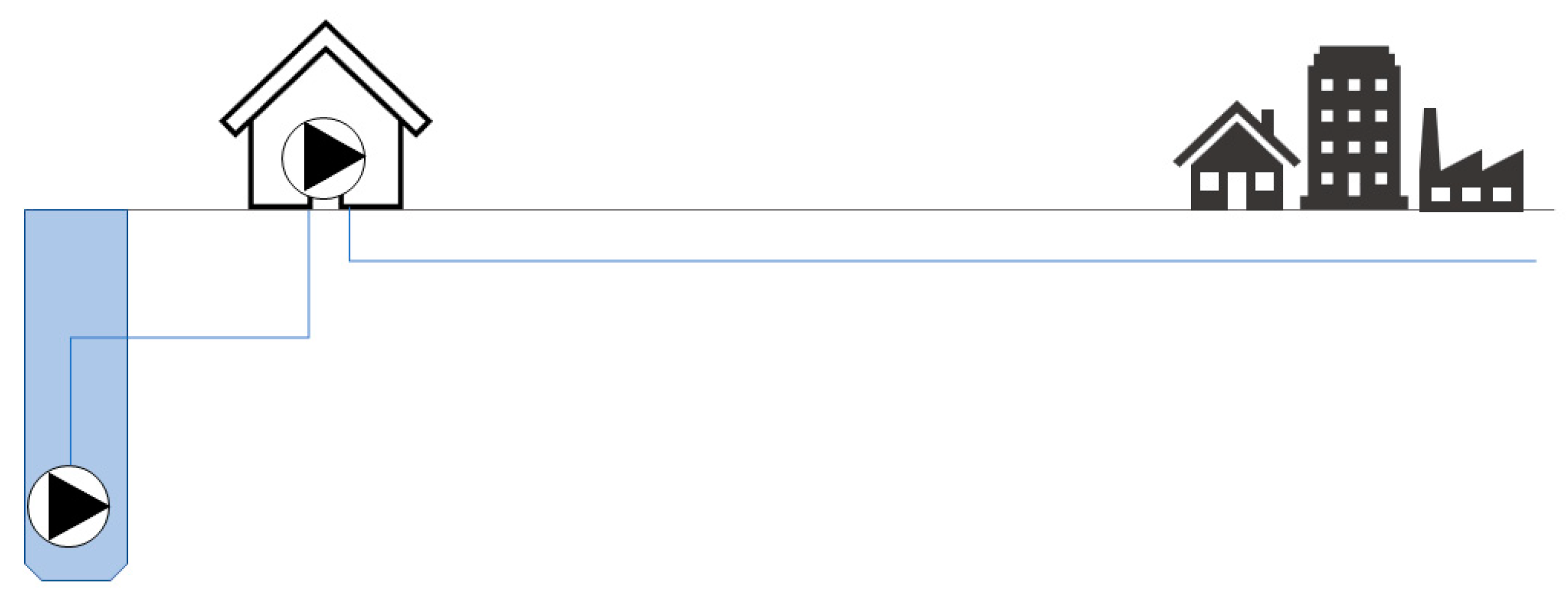
Gravity-Fed Systems (Figure 1) take advantage of the difference in height between where water is taken from the environment and where the consumer consumes it. An example of a Gravity-Fed System is the supply of a settlement unit from a field tank. Water to the tank can be supplied gravitationally from the intake (reservoirs like rivers or lakes), or it can be pumped from a well.
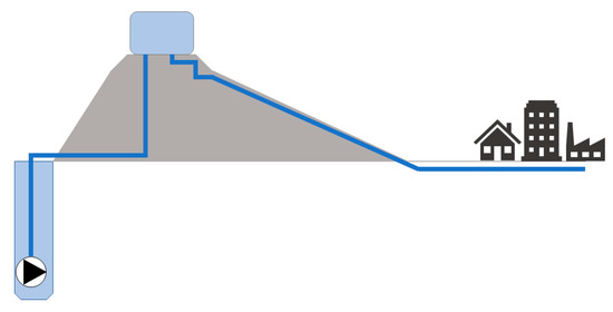
Figure 1.
Gravity-Fed Systems with pumps in the well to supply the water tank.
A Pumped System (Figure 2) requires the use of a water pump station (WPS), i.e., a building equipped with a set of pumps whose task is to increase the value of the pressure flowing into the WPS to deliver water to a settlement unit located far away, or located higher than the WPS.
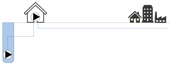
Figure 2.
Pumped systems with pumps in the well and the water pump station (WPS).
To reduce the energy consumption and operation of the WPS, a pumped system with field (intermediate) tanks is used, filled during hours of low water consumption by residents, and this supplements the work of the WPS during the peak hours of water consumption [5]. They allow for a reduction in the amount of pumped water.
A specific system is a long-distance and high-drop gravitational water supply system (LHGWSS), which requires the design of multiple pumping stations, an Energy Dissipation Box (EDB), and other factors [6]. In Poland, such a system can be found in Upper Silesia, where many towns and villages use LHGWSS to provide water to residents.
The existing WDS, despite the characteristics of the terrain sometimes allowing the use of the Gravity-Fed System, requires the construction of a WPS. The pressure losses from the water intake to the consumer are influenced by the pipe diameter, roughness, age (pipe aging, which in extreme cases can reduce the pipe diameter by a few dimensions), and flow rate [7,8]. The history of the location of a given section is also essential because pipes on the outskirts or in a branched system usually have smaller diameters, and their overgrowth—leading to an increase in roughness—occurs faster [7].
Reducing the consumption of electricity used in water pumping processes requires optimizing the selection of devices, optimizing operation (rules of control, for example, work schedules [9], systems of cooperation of objects [10]), and increasing the efficiency of pump operation. The optimization of the process of a WPS and pumps at water intakes, is necessary because they account for a large part of the costs of the entire WDS operation [11,12].
Optimizing the operation of a water pumping station is not only about the operation of the pumping station itself. Operation optimization begins at the stage of reducing water and energy losses in the distribution system. Water losses can be reduced with regard to real losses, where we reduce the number of failures or the duration of a single failure, or apparent losses, where we introduce more accurate water meters and remote reading systems [13]. Reducing energy losses involves, among other things, the appropriate selection of pipe diameters, e.g., the use of computer methods and artificial neural networks [14,15].
Attempts are made to reduce electricity consumption by optimizing the operation of pumping stations using Genetic Algorithm Optimization (GAO) [11], and especially the use of Simple Genetic Algorithms (SGA), Hybrid Genetic Algorithms (HGA), and Artificial Neural Networks (ANN) [16,17,18,19]. An adequately designed pumping system, selected pumps, and the application of the principles to minimize capital expenditures (CAPEX) and operating expenses (OPEX) allow us to reduce the WPS costs [10]. The use of variable speed pumps (VSPs) (rather than fixed speed pumps (FSPs)) leads to significant savings in both total costs [17]. The use of a VPS instead of an FPS reduces electricity consumption and thus reduces GHG emissions [20]. VSPs are increasingly used in WPS pump sets, but FSP pumps are most often used in intake wells—a small number of managers of water supply companies pay attention to optimizing water intakes. Most water supply companies focus on optimizing the water distribution process to consumers, not the process of water intake and delivery to the tank/water treatment plant.
A popular way to reduce the cost of electricity purchase is the use of renewable energy sources (photovoltaic installations [21], wind turbines [22]) or alternative forms of energy production using the flow of water in the water supply network (hydropower technology [23] or the Pumps As Turbine (PAT)) [24]. More and more often, PV installations are used to reduce the costs of pumping water and to supply WPS with electricity [25,26]. WPS researchers and operators recognize the need to monitor the production and consumption of electricity in WPS and PV installations [27].
Research on the use of PV installations to supply water pumps is carried out mainly in rural areas and water pumping stations used in agriculture [28]. A distributed WPS equipped with photovoltaic systems intergraded with a solar tracking system yields better performance and is more advantageous compared with a non-tracking system [29]. Tracking can be optimized using a new hybrid FL-INC optimization algorithm for the solar water pumping system [30]. The use of Artificial Neural Networks (ANNs) mathematical modeling has allowed to us predict the power generated in the photovoltaic installation for up to 3 h of pumping water in agriculture [31].
The use of solar panels and photovoltaic installations in Poland is justified [32,33]. The radiant energy value in Poland varies from 800 to 1100 W·m−2 per year. Insolation in Poland ranges from 1100 to 1300 kWh·m−2·year−1, depending on the region [23]. These values are comparable to those achieved in Germany, and about 20% lower than in Rome (1550 m−2·year−1) [34]. Poland has an average of 66 sunny days per year [35]. The insolation varies from 500 to 1300 h per quarter, depending on the season [36]. The highest electricity production from PV falls in the spring and summer, and in the winter (especially in December), it drops to close to zero. This is due to many cloudy days, short days, the distance from the equator, and thus the angle of incidence of rays on the surface of solar panels [37].
The research aims to check the possibility of reducing the costs of pumping water using a WPS by installing a low-power photovoltaic installation. The available area allows for the construction of PV installations with a power of 3.0 kW to 6.0 kW (variants with a power of 3.0 kW, 4.2 kW, and 6.0 kW were selected for the analysis). The tests were carried out on an existing pumping station and an existing 3.0 kW PV installation. Data recorded every hour were subject to the analysis of electricity production and consumption, with the latest flows for the year. In the conducted research, the authors attempted to check to what extent the production of electricity from the proposed variants of the PV installation will cover the current demands of WPS for electricity.
2. Materials and Methods
The tested water intake setup consists of a well equipped with a multi-stage constant-speed pump. The intake supplies water to one of the reservoirs that gravitationally supplies Polanica-Zdrój. The height difference between the intake and the reservoir is 50 m, and the distance is about 2 km. A water meter with a connected telemetry data logger is installed in the WPS. Flow data were recorded at 15-minute intervals.
Simulations and analyses were carried out for three power variants of photovoltaic installations. These variants are marked:
- PV 3.0 kW—installation with a power of 3.0 kW consisting of 10 panels with a power of 300 W each;
- PV 4.2 kW—installation with a power of 4.2. kW consisting of 14 panels with a power of 300 W each;
- PV 6.0 kW—installation with a power of 6.0 kW consisting of 20 panels with a power of 300 W each.
The basis for determining the production of electricity from individual variants of the installation was the energy produced in the existing 3.0 kW PV installation in Polanica-Zdrój, and the energy production was calculated on this basis using 1 panel with a power of 300 W (Formula (1)).
EPV I—simulated energy for a PV installation with power i, kW;
EPV—energy produced by the existing PV installation with a capacity of 3.0 kW, kW;
i—power of the simulated PV installation, kW;
n—number of panels in the existing installation with a capacity of 3.0 kW;
m—number of panels in the installation with power I.
In the article, we use two terms, sunny day and cloudy day. They mean:
- sunny day—a day with little cloudiness, on which the most energy was produced at the PV installation in a given month;
- cloudy day—a day with heavy cloudiness, on which the least energy was produced at the PV installation in a given month.
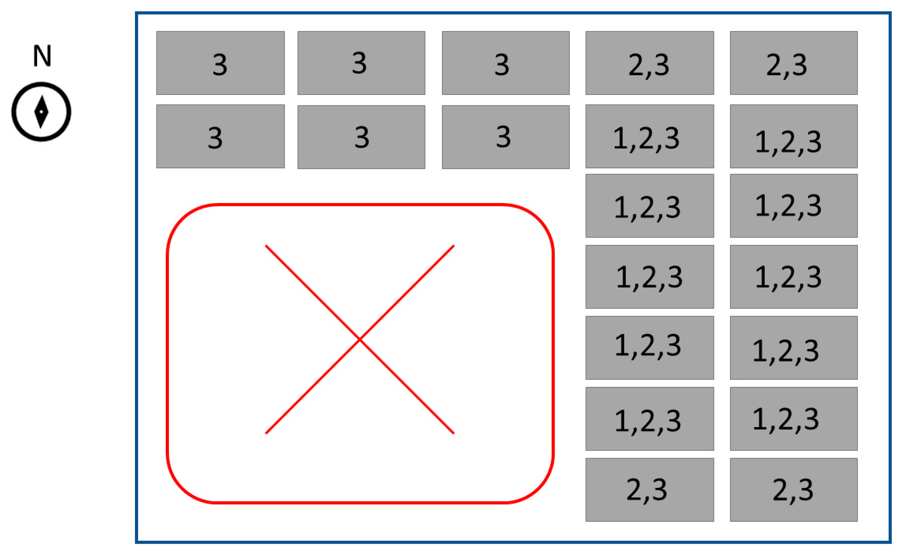
The surface and shape of the plot on which the water intake well with a pump is located allow for the assembly of panels in variants of 10, 14, and 20 pieces. The arrangement of the panels on the plot is shown in Figure 3.
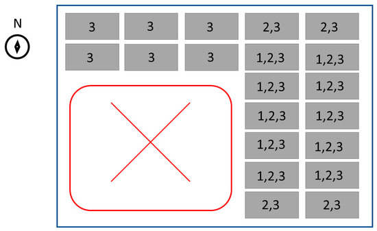
Figure 3.
Diagram of the arrangement of PV panels on the water intake plot (1—PV 3.0 kW variant, 2—PV 4.2 kW variant, 3—PV 6.0 kW variant).
The research included the following stages:
- Data collection and analysis of results from the existing 3.0 kW installation in Polanica-Zdrój;
- Collection of data and analysis of results on water production and electricity consumption in WPS;
- Measurements of the size and possibility of installing PV panels on the WPS plot;
- Analysis of electricity production and coverage of WPS demand for electricity from selected variants of PV installation power (3.0 kW, 4.2 kW, 6.0 kW).
The non-uniformity index of the pumped water was calculated using Formula (1) [38] and data were measured on the water meter in WPS.
where:
- Nt,a—non-uniformity index (−);
- Qt,a—amount of water pumped into the water supply network over time t (m3/t);
- Qt mean—mean amount of water pumped into the water supply network over time t (m3/t);
- t—a unit of time (month, day, hour)
- a—discriminant of the maximum or minimum index for a given unit of time, t.
3. Results and Discussion
3.1. Production of Energy from the Tested Installation with a Capacity of 3.0 kW in Seasons
3.1.1. Cloudy Days
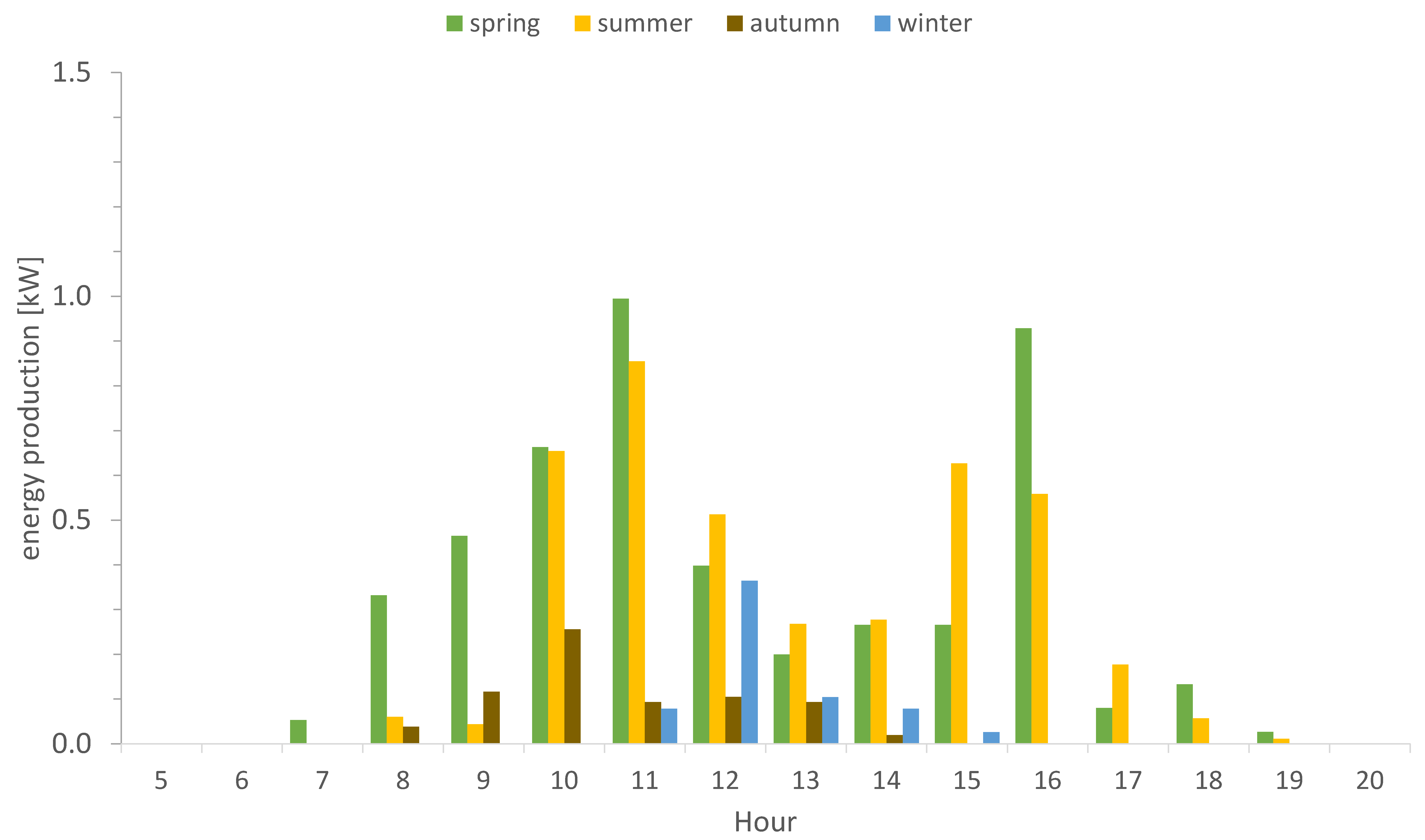
One cloudy day from the middle month of each of the four quarters (spring, summer, autumn, and winter) of 2021 was selected for the analysis. Figure 4 shows the value of energy produced for a given hour on each of the analyzed days of the quarters.
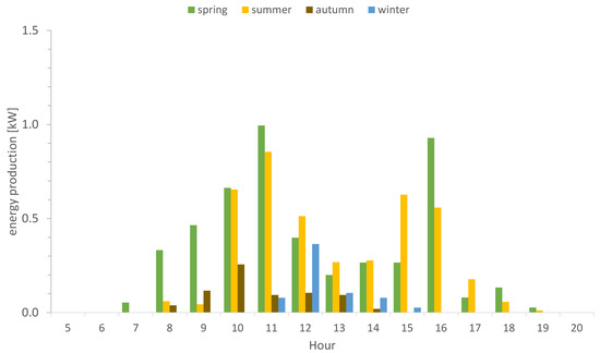
Figure 4.
Energy production on cloudy days from the tested installation (3.0 kW).
Spring energy production starts at 7 a.m. and ends around 7 p.m. On the analyzed day, the peak production power fell at 11 a.m. and 4 p.m. and reached the value of almost 1.00 kWh.
In summer, energy production starts at 8 a.m. and ends around 7 p.m. On the analyzed day, the peak production power fell at 11 a.m. and reached the value of about 0.85 kWh.
In autumn, energy production starts at 8 a.m. and ends around 2 p.m. On the analyzed day, the peak production power fell at 10 a.m. and reached the value of 0.26 kWh.
In winter, energy production starts at 11 a.m. and ends around 3 p.m. On the analyzed day, the peak production power fell at noon and reached the value of 0.36 kWh.
3.1.2. Sunny Days
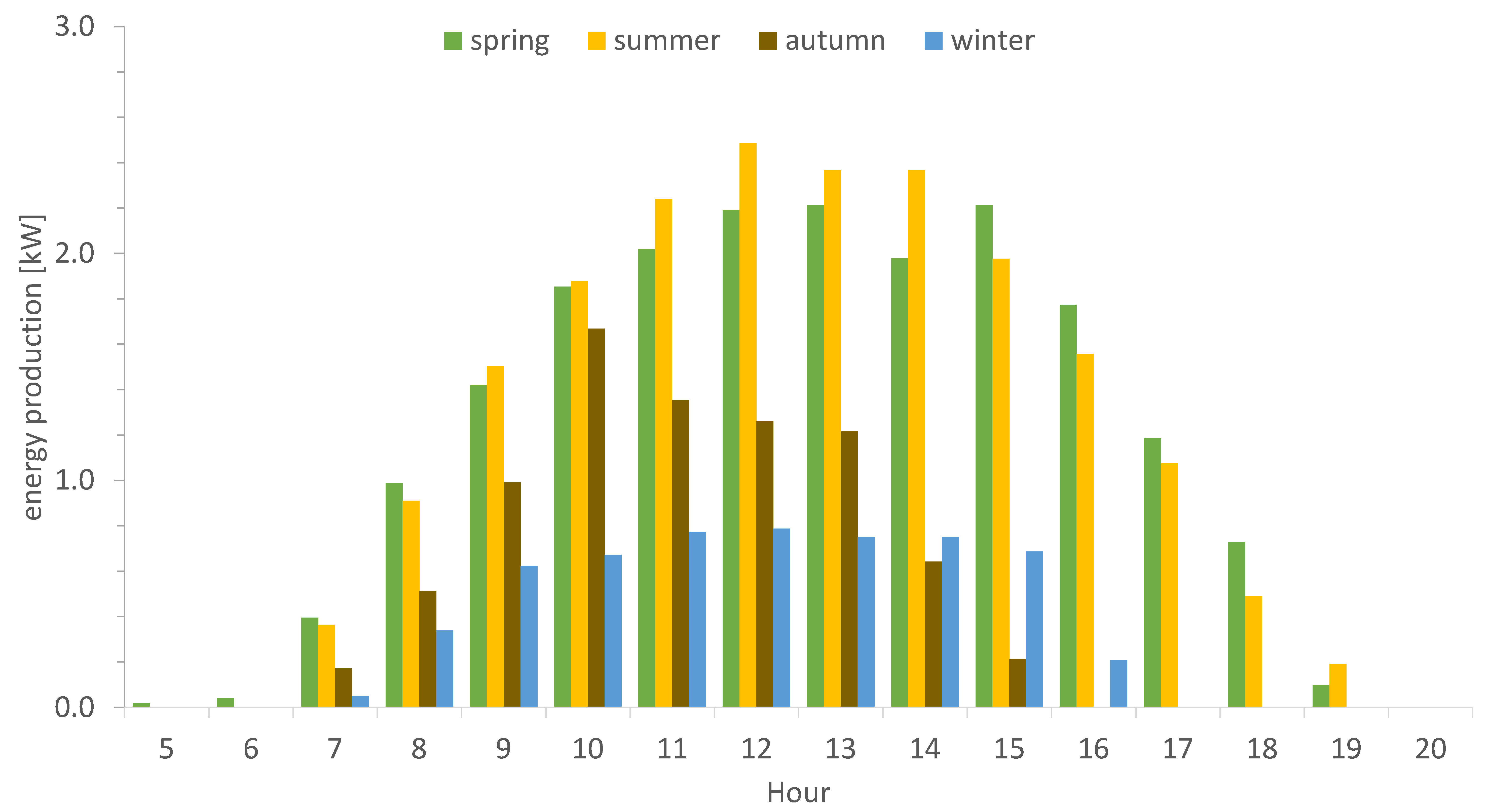
One sunny day from the middle month of each of the four quarters (spring, summer, autumn, winter) of 2021 was selected for the analysis. Figure 5 shows the value of energy produced for a given hour on each of the analyzed days of the quarters.
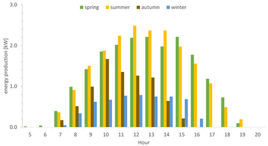
Figure 5.
Energy production on sunny days from the tested installation (3.0 kW).
In spring, energy production starts at 5 a.m. and ends around 7 p.m. On the analyzed day, the peak production power fell at 1 p.m. and reached the value of almost 2.21 kWh. From 11 a.m. to 3 p.m., more than 2.00 kWh was produced each hour.
In summer, energy production starts at 7 a.m. and ends around 7 p.m. From 11 a.m. to 2 p.m., more than 2.00 kWh was produced each hour. On the analyzed day, the peak production power fell at noon and reached the value of about 2.49 kWh.
In autumn, energy production starts at 7 a.m. and ends around 3 p.m. On the analyzed day, the peak production power fell at 10 a.m. and reached the value of 1.67 kWh.
In winter, energy production starts at 7 a.m. and ends around 4 p.m. From 11 a.m. to 2 p.m., over 0.75 kWh was produced each hour. On the analyzed day, the peak production power fell at noon and reached the value of 0.79 kWh.
3.1.3. Daily Production
The minimum and maximum daily electricity productions from the tested installation with a capacity of 3.0 kW are shown in Table 1. The installation produced less than 3.0 kW in January, February, April, June, September, October, November, and December. In December, days were observed when the installation did not produce energy. The minimum level (close to zero) was also recorded in November. The highest minimum value of daily energy production from PV installations was in July, i.e., 5.17 kWh.

Table 1.
Minimum and maximum daily production of electricity from the tested installation (3.0 kW).
In December, the maximum daily electricity production did not exceed 1 kWh. In the remaining months, the total daily energy production exceeded 3.0 kWh. In November, it amounted to 3.25 kWh. The highest daily electricity output was recorded in June (20.57 kWh). In June and July, the daily production increased by more than 20 kWh. From March to August, the maximum daily electricity production was three times the installation’s capacity (i.e., production greater than 18.0 kWh per day).
3.2. Water Production and Its Unevenness during the Day and Year (Monthly)
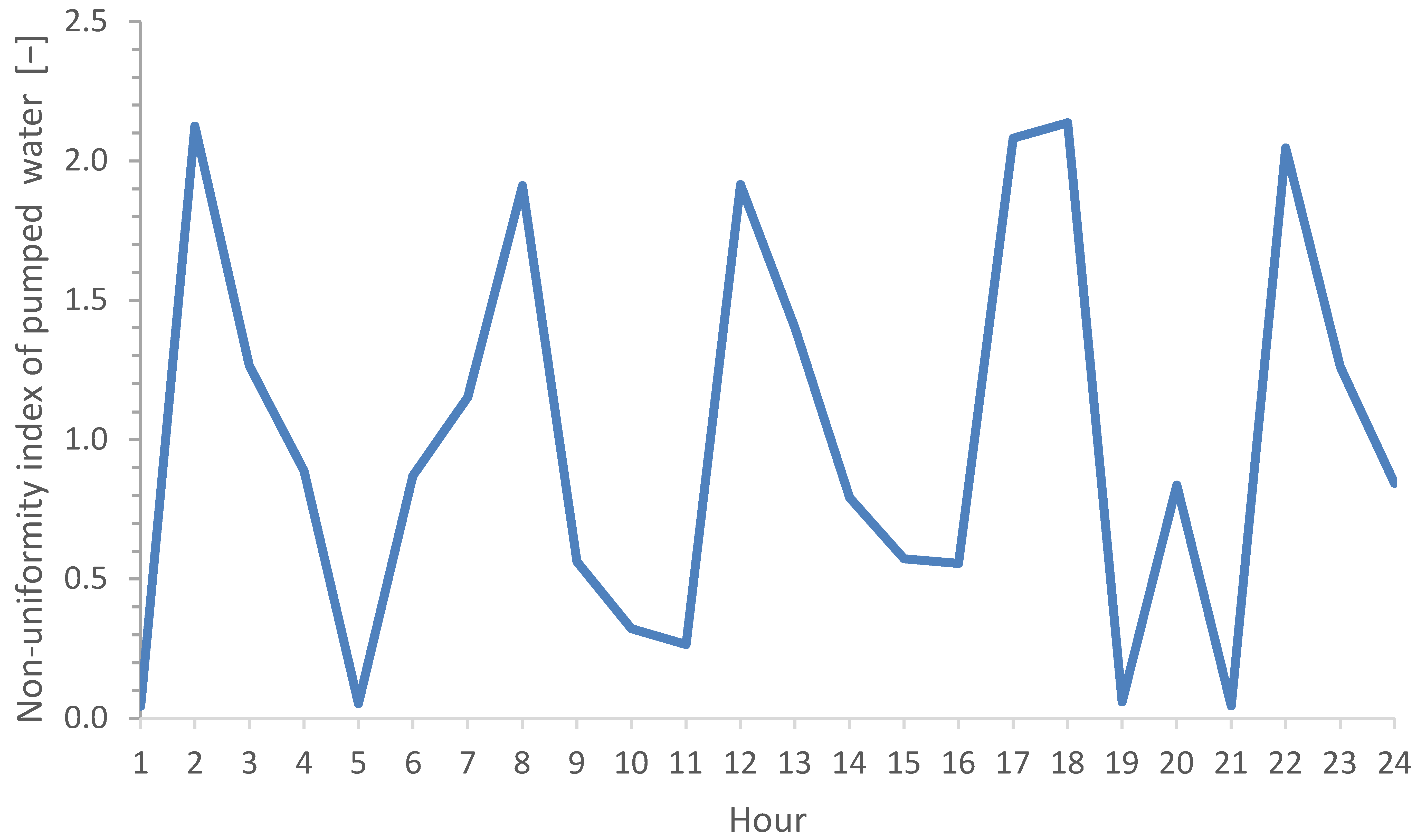
The characteristics of pump operation at the water intake are presented in the form of indicators of hourly water pumping irregularity in Figure 6. The features of filling the reservoir from the information and water intake by the settlement unit require four periods of water replenishment in the pool: from midnight to 4 a.m., from 4 a.m. to 6 p.m., from 6 p.m. to 8 p.m., and from 8 p.m. to midnight. In the second period, there are three moments of increased water pumping into the tank and two moments of reduced efficiency of water pumping into the tank.
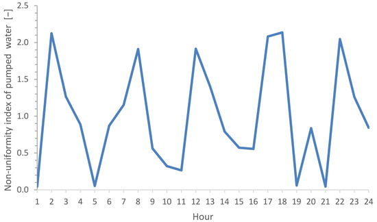
Figure 6.
Hourly non-uniformity index of pumped water during the day.
The variability of the amount of water pumped into the reservoir in a given month during the year is presented as an indicator of monthly water pumping irregularity in Figure 7. The nature of the settlement caused a significant increase in water demand in the period from May to October. The highest demand falls in the summer period from July to September (above 2.5 of the average monthly water consumption).
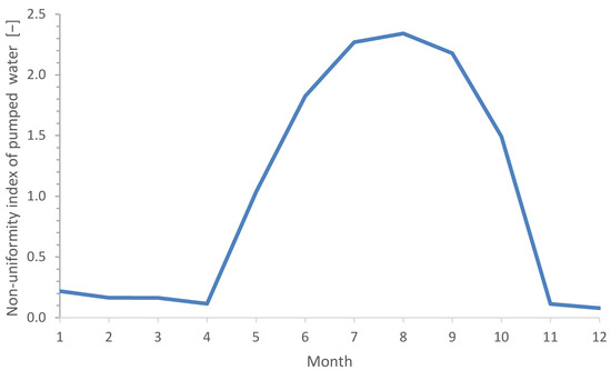
Figure 7.
Monthly non-uniformity index of pumped water during the year.
3.3. Demand for Energy about Production from Installation Variants
The electricity consumed by the pump pumping water into the tank is shown in Figure 8. The pump’s electricity consumption strongly depends on the work involved and the amount of water pumped from the well to the tank. In the period from May to October, there is the highest water consumption in the settlement unit, which directly translates into energy consumption. The tests on the facility also show that the frequency of pump operation and the value of work (the value of the head and flow) affect the achieved values of electricity consumption for pumping 1 m3 of water to the tank. The electricity consumption for pumping 1 m3 of water is presented in Table 2. The average electricity consumption for pumping 1 m3 of water varies from 0.233 kWh·m−3 to 0.544 kWh·m−3. The minimum electricity consumption for pumping 1 m3 of water differs from 0.161 kWh·m−3 to 0.408 kWh·m−3. The maximum electricity consumption for pumping 1 m3 of water varies from 0.331 kWh·m−3 to 0.762 kWh·m−3.
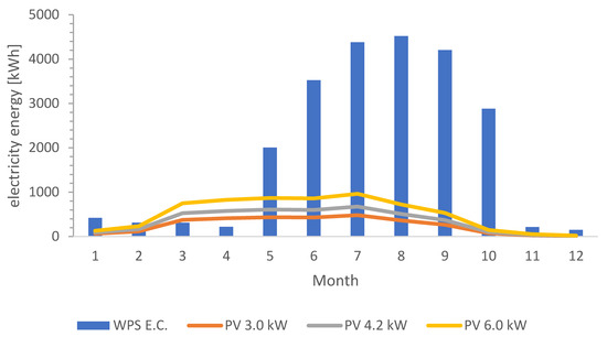
Figure 8.
Electricity production by 3.0 kW, 4.2 kW, and 6.0 kW installations and water pump station electricity consumption (WPS E.C.).
Table 2.
Pumping system consumption of electricity index—EC (kWh·m−3).
An analysis of electricity production from various installations with the power of 3.0 kW, 4.2 kW, and 6.0 kW was made. The energy production values from the proposed system were determined based on tests carried out on a simple installation with a capacity of 3 kW installed in the analyzed settlement and the converted values that could be achieved in the case of expanding the installation to 4.2 kW and 6.0 kW. The simulated energy production values are presented in Figure 8. The total energy production from the variant PV installations exceeded the total monthly energy consumption of the pump only in March and April. In the remaining months, the full value of the monthly energy production from the PV installation in each variant is lower than the total value of energy consumed by the facility. From March to September, the monthly energy production by each analyzed PV installation variant is higher than the average monthly production for the year. From October to February, the value of energy production from each analyzed PV installation is lower than the average monthly production for the year.
3.4. Analysis of Demand Coverage in a Given Month
The coverage of the total monthly electricity demand of the facility in relation to the energy produced by the PV installation in individual variants was analyzed (Table 3).
Table 3.
The total monthly percentage coverage of the pump’s demand for electricity from a kW installation.
The 3.0 kW PV variant provides only 13.2% of the pump station’s total demand during the year. The total monthly production of the complete monthly request ranges from 2.6% in October to 185.1% in April. In March and April, the total monthly production covers over 100% of the monthly electricity demand. In other months, this ratio is lower than 50%.
The 4.2 kW PV variant provides only 18.5% of the building’s demand in total during the year. The total monthly production of the total monthly market covered from 3.6% in October to 259.1% in April. In March and April, the total monthly production covers over 100% of the monthly electricity demand. From February to April, the total monthly production covers more than 50% of the monthly electricity demand. In other months, this ratio is lower than 50%.
The 6.0 kW PV variant provides only 26.4% of the facility’s total demand during the year. The total monthly production of the total monthly market ranges from 5.2% in October to 370.1% in April. In March and April, the total monthly production covers over 100% of the monthly electricity demand. From February to April, the total monthly production covers more than 70% of the monthly electricity demand. In other months, this ratio is lower than 50%.
3.5. Hourly Analysis of Demand Coverage
An analysis of the coverage of the facility’s hourly demand for electricity in relation to the energy produced by the PV installation in a given hour in individual variants, months, and for a cloudy day and a sunny day is here carried out.
The analysis considers changes in the demand for water in a settlement unit during the year and during the day, changes in the average demand for electricity for pumping 1 m3 of water in a given month, and the distribution of hourly energy production for cloudy and sunny days.
The hourly analysis allows one to identify the hours and values of energy production and perform an actual comparison with the demand for energy in a given hour.
For cloudy days, the values of coverage of the hourly demand are:
- In the PV 3.0 kW variant—from 0.00% to 452.9%, an average of 16.5%;
- In the PV 4.2 kW variant—from 0.00% to 654.1%, an average of 23.2%;
- In the PV 6.0 kW variant—from 0.00% to 905.8%, an average of 33.1%.
For sunny days, the values of coverage of the hourly demand are:
- In the PV 3.0 kW variant—from 0.00% to 3220.2%, on average, 105.3%;
- In the PV 4.2 kW variant—from 0.00% to 4508.3%, an average of 147.4%;
- In the PV 6.0 kW variant—from 0.00% to 6440.4%, on average, 210.6%.
In the next step, an analysis is made of hours when no energy is produced, hours with energy production from 0.00% to 100% of the demand, and hours with an output of more than 100% of the energy demand for pump operation.
For cloudy days, the value of covering the hourly demand is:
- in the PV 3.0 kW variant—34.7% of hours per year with energy production up to 100% of the demand, 3.8% of hours with energy production over 100% of the annual demand;
- In the PV 4.2 kW variant—31.6% of hours per year with energy production up to 100% of the demand, 6.9% of hours with energy production over 100% of the annual demand;
- In the PV 6.0 kW variant—29.9% of hours per year with energy production up to 100% of the demand, 8.7% of hours with energy production over 100% of the annual demand.
For sunny days, the value of coverage of the hourly demand is:
- In the PV 3.0 kW variant—23.3% of hours per year with energy production up to 100% of the demand, 15.3% of hours with energy production over 100% of the annual demand;
- In the PV 4.2 kW variant—18.1% of hours per year with energy production up to 100% of the demand, 20.5% of hours with energy production over 100% of the annual demand;
- In the PV 6.0 kW variant—17.4% of hours per year with energy production up to 100% of the demand, 21.2% of hours with energy production over 100% of the annual demand.
Table 4 shows the total coverage of the facility’s electricity demand based on hourly energy production in individual PV installation variants for each month of the year in the case of cloudy days. Coverage of the total hourly demand by the total hourly output on cloudy days in each month varies:
Table 4.
The total day percentage coverage of the pump demand for electricity from the photovoltaic installation for cloudy days.
- From 0.0% to 35.8% for the 3.0 kW PV variant;
- From 0.0% to 40.0% for the 4.2 kW PV variant;
- From 0.0% to 42.7% for the 6.0 kW PV variant.
Table 5 presents the total coverage of the facility’s electricity demand based on the hourly energy production in individual variants of the PV installation for each month of the year in the case of sunny days. Coverage of the total hourly demand by the total hourly production on cloudy days in each month changes:
Table 5.
The total day percentage coverage of the pump demand for electricity from the photovoltaic installation for sunny days.
- From 11.3% to 46.8% for the 3.0 kW PV variant;
- From 15.1% to 48.9% for the 4.2 kW PV variant;
- From 17.6% to 52.0% for the 6.0 kW PV variant.
Table 6 shows the percentage share of overproduction of electricity in relation to the total daily electricity production in a given variant of the PV installation for a cloudy day. Overproduction is understood as the value of electricity produced in a given hour above the value of WPS electricity demand.
Table 6.
The percentage share of overproduction of electricity in relation to the total daily electricity production in a given variant of the PV installation for a cloudy day.
The overproduction of electricity from the PV installation with regard to the energy produced by the installation on cloudy days changes:
- From 0.0% to 19.2% for the PV 3.0 kW variant;
- From 0.0% to 32.1% for the 4.2 kW PV variant;
- From 0.0% to 47.9% for the 6.0 kW PV variant.
The overproduction of energy above the WPS demand in a given hour occurs only from February to April in each variant (on cloudy days).
Table 7 shows the percentage share of overproduction of electricity in relation to the total daily electricity production in a given variant of the PV installation for a sunny day. Overproduction is understood as the value of electricity produced above the value of demand for electricity WPS in a given hour.
Table 7.
The percentage share of overproduction of electricity in relation to the total daily electricity production in a given variant of the PV installation for a sunny day.
The overproduction of electricity from the PV installation with regard to the energy produced by the installation on sunny days changes:
- From 7.2% to 82.9% for the 3.0 kW PV variant;
- From 11.9% to 86.8% for the 4.2 kW PV variant;
- From 18.1% to 89.8% for the 6.0 kW PV variant.
Overproduction of energy over the WPS demand at a given hour occurs throughout the year in every variant (on sunny days).
4. Conclusions
Using RES in water pumping stations or water intake wells allows one to generate savings related to the provision of electricity for pump operation. Providing results showing the total annual production and comparing it with the total annual demand of pumps makes owners or operators more willing to use such a solution. The amount of electricity produced by a PV installation depends on its size (number of panels). In the case of micro installations on small objects, the profits are not as impressive as in the case of larger installations (12 kW–40 kW) [39,40]. In the analyzed case, the top variant of the PV installation is 6.0 kW, which translates to providing from 15.3 to 48.9% of the daily energy demand. The analysis of profitability or ensured self-sufficiency of a water supply facility should be carried out based on a minimum of hourly data on energy production and demand [40]. The study then shows the actual coverage of demand by production. The energy produced that exceeds the demand will either be stored or resold to the power grid.
It should be remembered that the price of fuel sold and the cost of energy purchased from the power grid is not the same. In the article, it was not decided to conduct economic analyses based on changes in energy purchase and sales prices because electricity prices have been subject to such strong fluctuations in recent periods (energy prices on the market, prices of raw materials, legislative works, new regulations, armed conflicts) that the presented price effects would distort the image of the entire process of balancing the production and consumption of electricity by the water pumping station (self-consumption).
Using a PV installation as a remedy for energy consumption by pumps is not a solution in itself that will allow for a reduction in the purchase of energy from the grid. Still, it will not solve the problem of high energy consumption by pumps. PV installations can be a good solution, but only after applying the correct selection of pumps, devices, and control methods. Only then should the guarantee of energy supplies from RES be taken care of. The results and conclusions we obtain can be used to further research on and the optimization of the processes of selecting the optimal pump size, pump operation schedules, or pump operation control similar to research carried out on larger facilities with a different work structure [26,30,31], as well as the modernization of water distribution systems: the renovation of pipes or cooperation of the pumping station with the reservoir. The obtained results relate to a PV installation with a permanent structure facing south. We were not able to check the influence of the direction of construction and the angle of inclination of the panels on the amount of electricity produced. This is the basis for further research and the attempt to find an optimal solution to ensure the self-consumption of energy from RES in the case of water pumping.
Author Contributions
Conceptualization, K.Ś., M.Ś., M.K. and J.G.-M.; formal analysis, K.Ś., M.Ś., M.K. and J.G.-M.; methodology, K.Ś., M.Ś., M.K. and J.G.-M.; writing, M.Ś. and M.K.; writing—review and editing, K.Ś. and J.G.-M. All authors have read and agreed to the published version of the manuscript.
Funding
This research was funded by the Polish National Centre for Research and Development, under grant no. POIR.01.01.01.-00-1818/20 “Intelligent Water Supply Network–Municipal Data Platform”.
Data Availability Statement
Data will be made available on request.
Conflicts of Interest
The authors declare that they have no known competing financial interests or personal relationships that could have appeared to influence the work reported in this paper.
References
- De Corte, A.; Sörensen, K. Optimisation of Gravity-Fed Water Distribution Network Design: A Critical Review. Eur. J. Oper. Res. 2013, 228, 1–10. [Google Scholar] [CrossRef]
- Burgschweiger, J.; Gnädig, B.; Steinbach, M.C. Optimization Models for Operative Planning in Drinking Water Networks. Optim. Eng. 2009, 10, 43–73. [Google Scholar] [CrossRef]
- Słowiński, R. A Multicriteria Fuzzy Linear Programming Method for Water Supply System Development Planning. Fuzzy Sets Syst. 1986, 19, 217–237. [Google Scholar] [CrossRef]
- Verleye, D.; Aghezzaf, E.-H. Modeling and Optimization of Production and Distribution of Drinking Water at VMW. In Proceedings of the Network Optimization, Hamburg, Germany, 13–16 June 2011; Pahl, J., Reiners, T., Voß, S., Eds.; Springer: Berlin/Heidelberg, Germany, 2011; pp. 315–326. [Google Scholar]
- Thornton, J.; Sturm, R.; Kunkel, G. (Eds.) Water Loss Control, 2nd ed.; McGraw-Hill Education: New York, NY, USA, 2008; ISBN 978-0-07-149918-7. [Google Scholar]
- Ni, W.; Zhang, J.; Chen, S. Optimal Location of Energy Dissipation Box in Long Distance and High Drop Gravitational Water Supply System. Water 2021, 13, 461. [Google Scholar] [CrossRef]
- Hashemi, S.; Filion, Y.; Speight, V.; Long, A. Effect of Pipe Size and Location on Water-Main Head Loss in Water Distribution Systems. J. Water Resour. Plan. Manag. 2020, 146, 06020006. [Google Scholar] [CrossRef]
- Wichowski, P.; Kalenik, M.; Lal, A.; Morawski, D.; Chalecki, M. Hydraulic and Technological Investigations of a Phenomenon Responsible for Increase of Major Head Losses in Exploited Cast-Iron Water Supply Pipes. Water 2021, 13, 1604. [Google Scholar] [CrossRef]
- Alvisi, S.; Franchini, M. A Methodology for Pumping Control Based on Time Variable Trigger Levels. Procedia Eng. 2016, 162, 365–372. [Google Scholar] [CrossRef]
- Gutiérrez-Bahamondes, J.H.; Mora-Meliá, D.; Iglesias-Rey, P.L.; Martínez-Solano, F.J.; Salgueiro, Y. Pumping Station Design in Water Distribution Networks Considering the Optimal Flow Distribution between Sources and Capital and Operating Costs. Water 2021, 13, 3098. [Google Scholar] [CrossRef]
- Dadar, S.; Đurin, B.; Alamatian, E.; Plantak, L. Impact of the Pumping Regime on Electricity Cost Savings in Urban Water Supply System. Water 2021, 13, 1141. [Google Scholar] [CrossRef]
- Blinco, L.J.; Simpson, A.R.; Lambert, M.F.; Auricht, C.A.; Hurr, N.E.; Tiggemann, S.M.; Marchi, A. Genetic Algorithm Optimization of Operational Costs and Greenhouse Gas Emissions for Water Distribution Systems. Procedia Eng. 2014, 89, 509–516. [Google Scholar] [CrossRef]
- Cichoń, T.; Królikowska, J. Remote Reading of Water Meters as an Element of a Smart City Concept. Rocz. Ochr. Śr. 2021, 23, 883–890. [Google Scholar] [CrossRef]
- Dawidowicz, J. The Concept of Calculating the Water Distribution System as a Repeatable Process with Elements of Diagnostics Using Neural Modeling. Rocz. Ochr. Śr. 2022, 24, 493–504. [Google Scholar] [CrossRef]
- Gvishiani, Z.; Dawidowicz, J. Comparison of MLP and RBF Neural Networks in the Task of Classifying the Diameters of Water Pipes. Rocz. Ochr. Śr. 2022, 24, 505–519. [Google Scholar] [CrossRef]
- Ramos, H.M.; Costa, L.H.M.; Gonçalves, F.V.; Ramos, H.M.; Costa, L.H.M.; Gonçalves, F.V. Energy Efficiency in Water Supply Systems: GA for Pump Schedule Optimization and ANN for Hybrid Energy Prediction; IntechOpen: London, UK, 2012; ISBN 978-953-51-0889-4. [Google Scholar]
- Wu, W.; Simpson, A.R.; Maier, H.R.; Marchi, A. Incorporation of Variable-Speed Pumping in Multiobjective Genetic Algorithm Optimization of the Design of Water Transmission Systems. J. Water Resour. Plan. Manag. 2012, 138, 543–552. [Google Scholar] [CrossRef]
- Feng, X.; Qiu, B.; Wang, Y. Optimizing Parallel Pumping Station Operations in an Open-Channel Water Transfer System Using an Efficient Hybrid Algorithm. Energies 2020, 13, 4626. [Google Scholar] [CrossRef]
- Cimorelli, L.; Covelli, C.; Molino, B.; Pianese, D. Optimal Regulation of Pumping Station in Water Distribution Networks Using Constant and Variable Speed Pumps: A Technical and Economical Comparison. Energies 2020, 13, 2530. [Google Scholar] [CrossRef]
- Mala-Jetmarova, H.; Sultanova, N.; Savic, D. Lost in Optimisation of Water Distribution Systems? A Literature Review of System Design. Water 2018, 10, 307. [Google Scholar] [CrossRef]
- Kazem, H.A.; Quteishat, A.; Younis, M.A. Techno-Economical Study of Solar Water Pumping System: Optimum Design, Evaluation, and Comparison. Renew. Energy Environ. Sustain. 2021, 6, 41. [Google Scholar] [CrossRef]
- Koulouri, A.; Moccia, J. Saving Water with Wind Energy; The European Wind Energy Association (EWEA): Brussels, Belgium, 2014. [Google Scholar]
- Sari, M.A.; Badruzzaman, M.; Cherchi, C.; Swindle, M.; Ajami, N.; Jacangelo, J.G. Recent Innovations and Trends in In-Conduit Hydropower Technologies and Their Applications in Water Distribution Systems. J. Environ. Manag. 2018, 228, 416–428. [Google Scholar] [CrossRef]
- Sambito, M.; Piazza, S.; Freni, G. Stochastic Approach for Optimal Positioning of Pumps As Turbines (PATs). Sustainability 2021, 13, 12318. [Google Scholar] [CrossRef]
- Đurin, B.; Margeta, J. Analysis of the Possible Use of Solar Photovoltaic Energy in Urban Water Supply Systems. Water 2014, 6, 1546–1561. [Google Scholar] [CrossRef]
- Argaw, N. Renewable Energy Water Pumping Systems Handbook; Period of Performance: 1 April–1 September 2001; NREL/SR-500-30481; National Renewable Energy Lab. (NREL): Golden, CO, USA, 2004; p. 15008778. [Google Scholar]
- Gimeno-Sales, F.J.; Orts-Grau, S.; Escribá-Aparisi, A.; González-Altozano, P.; Balbastre-Peralta, I.; Martínez-Márquez, C.I.; Gasque, M.; Seguí-Chilet, S. PV Monitoring System for a Water Pumping Scheme with a Lithium-Ion Battery Using Free Open-Source Software and IoT Technologies. Sustainability 2020, 12, 10651. [Google Scholar] [CrossRef]
- Irandoostshahrestani, M.; Rousse, D.R. Photovoltaic Electrification and Water Pumping Using the Concepts of Water Shortage Probability and Loss of Power Supply Probability: A Case Study. Energies 2023, 16, 1. [Google Scholar] [CrossRef]
- Imjai, T.; Thinsurat, K.; Ditthakit, P.; Wipulanusat, W.; Setkit, M.; Garcia, R. Performance Study of an Integrated Solar Water Supply System for Isolated Agricultural Areas in Thailand: A Case-Study of the Royal Initiative Project. Water 2020, 12, 2438. [Google Scholar] [CrossRef]
- Hilali, A.; El Ouanjli, N.; Mahfoud, S.; Al-Sumaiti, A.S.; Mossa, M.A. Optimization of a Solar Water Pumping System in Varying Weather Conditions by a New Hybrid Method Based on Fuzzy Logic and Incremental Conductance. Energies 2022, 15, 8518. [Google Scholar] [CrossRef]
- Cervera-Gascó, J.; Perea, R.G.; Montero, J.; Moreno, M.A. Prediction Model of Photovoltaic Power in Solar Pumping Systems Based on Artificial Intelligence. Agronomy 2022, 12, 693. [Google Scholar] [CrossRef]
- Wicki, L.; Pietrzykowski, R.; Kusz, D. Factors Determining the Development of Prosumer Photovoltaic Installations in Poland. Energies 2022, 15, 5897. [Google Scholar] [CrossRef]
- Gnatowska, R.; Moryń-Kucharczyk, E. The Place of Photovoltaics in Poland’s Energy Mix. Energies 2021, 14, 1471. [Google Scholar] [CrossRef]
- Stryczewska, H.D. (Ed.) Energie Odnawialne: Przegląd Technologii i Zastosowań; Politechnika Lubelska: Lublin, Poland, 2012; ISBN 978-83-62596-84-3. [Google Scholar]
- Trzy Parametry, Które Powinien Znać Przyszły Prosument | Planergia. Available online: https://www.planergia.pl/post/trzy-parametry-ktore-powinien-znac-przyszly-prosument-1892 (accessed on 5 December 2022).
- Śmierzchalska, P.; Chmielowiec, M. Mapa Usłonecznienia w Polsce; Akademia Pomorska w Słupsku: Słupsk, Poland, 2015; 9p. [Google Scholar]
- Nowak, W.; Stachel, A. Kolektory słoneczne i panele fotowoltaiczne jako źródło energii w małych instalacjach cieplnych i elektroenergetycznych. Autom. Elektr. Zakłócenia 2011, 2, 55–64. [Google Scholar]
- Gwoździej-Mazur, J.; Świętochowski, K. Non-Uniformity of Water Demands in a Rural Water Supply System. J. Ecol. Eng. 2019, 20, 245–251. [Google Scholar] [CrossRef]
- Świętochowski, K.; Średziński, P.; Malmur, R.; Gwoździej-Mazur, J. Analysis of the Possibility of Energy Self-Sufficiency of Water Pumping Stations with the Use of PV Installations. Int. Commun. Heat Mass Transf. 2023, 143, 106683. [Google Scholar] [CrossRef]
- Średziński, P.; Świętochowska, M.; Świętochowski, K.; Gwoździej-Mazur, J. Analysis of the Use of the PV Installation in the Power Supply of the Water Pumping Station. Energies 2022, 15, 9536. [Google Scholar] [CrossRef]


Disclaimer/Publisher’s Note: The statements, opinions and data contained in all publications are solely those of the individual author(s) and contributor(s) and not of MDPI and/or the editor(s). MDPI and/or the editor(s) disclaim responsibility for any injury to people or property resulting from any ideas, methods, instructions or products referred to in the content. |
© 2023 by the authors. Licensee MDPI, Basel, Switzerland. This article is an open access article distributed under the terms and conditions of the Creative Commons Attribution (CC BY) license (https://creativecommons.org/licenses/by/4.0/).