Article

Compositional Simulation of CO2 Huff-n-Puff Processes in Tight Oil Reservoirs with Complex Fractures Based on EDFM Technology Considering the Threshold Pressure Gradient

1
Hubei Key Laboratory of Petroleum Geochemistry and Environment, Yangtze University, Wuhan 430100, China
2
The Fourth Oil Production Plant, PetroChina Changqing Oilfield Company, Yulin 718500, China
3
The Tenth Oil Production Plant, PetroChina Changqing Oilfield Company, Qingyang 745100, China
4
School of Earth Resources, China University of Geosciences, Wuhan 430074, China
*
Author to whom correspondence should be addressed.
Energies 2023, 16(22), 7538; https://doi.org/10.3390/en16227538
Submission received: 9 October 2023 / Revised: 8 November 2023 / Accepted: 9 November 2023 / Published: 12 November 2023
(This article belongs to the Section H: Geo-Energy)

Abstract

:
Although tight oil reservoirs have abundant resources, their recovery efficiency is generally low. In recent years, CO2 injection huff-n-puff has become an effective method for improving oil recovery on the basis of depleted production of volume-fracturing horizontal wells in tight oil reservoirs. In order to study the effects of CO2 huff-n-puff (CO2-HnP) on production, a compositional numerical simulation study of CO2 huff-n-puff (CO2-HnP) was conducted in tight oil reservoirs with complex fractures. Embedded discrete fracture model technology was used in the simulations to characterize complex fractures. The process of CO2 huff-n-puff (CO2-HnP) was simulated, which consists of CO2 injection, CO2 soaking, and CO2 production. Taking into account the threshold pressure gradient and stress sensitivity in the model, we conducted a series of numerical simulations with different production condition parameters, such as bottom-hole pressure, CO2 injection rate, injection time, soaking time, and the number of cycles of CO2 huff-n-puff (CO2-HnP). Then, the effects of these sensitivity parameters on the cumulative oil production (COP) were studied. The results indicate that the threshold pressure gradient and rock stress sensitivity factors greatly affect the pressure field of tight reservoirs and the cumulative oil production (COP) of multistage-fracturing horizontal wells. The production parameters all have an impact on the COP. The injection rate and circulation number both have optimal values, and the injection time and soak time tend to have less significant effects on the growth of cumulative oil production over time. According to the numerical simulation, the optimal solution is 5 × 10⁴ m3/day injection rate per cycle, 25 days of injection time, 35 days of soaking time, three cycles, and production for 5 years, which can obtain the optimal cumulative oil production.

1. Introduction

Tight oil reservoirs are becoming a global hotspot in oil resource exploration and development. Although tight oil reservoirs have abundant resources, their recovery efficiency is generally low. The global average recovery rate of natural depletion development in tight oil reservoirs is only 3 to 10% [1,2,3]. How to improve the recovery efficiency in tight oil reservoirs has become a difficult problem that needs to be continuously addressed.
Improving the recovery rate of tight oil reservoirs requires reservoir densification and reservoir energy enhancement to enhance the fluid mobility in tight formations. Reservoir densification is a reservoir transformation method that benefits from the technology of volume fracturing and horizontal wells, which are used to increase the movable oil area and improve the permeability of tight reservoirs. Multistage hydraulic fracturing has become the main technology for extracting tight oil and has achieved significant results [4]. Many tight formation outcrops, cores, and image logs have confirmed the existence of natural fractures or fracture traces [5,6]. Hydraulic fracturing establishes fracture fairways, which interact with natural fracture systems [7]. Because the presence of fractures and the geometry of the fracture networks significantly affect the flow behavior, it is crucial to accurately simulate realistic fractures with complex geometric shapes, as well as the influence of fractures on well productivity [8]. Due to the complexity of fracture geometry, several approaches have been proposed to simulate fracture networks. There are generally two types of models to simulate complex fractures, i.e., dual-continuum and discrete fracture models (DFMs) [9].
Dual-continuum models are the conventional method, first introduced by Barenblat et al. (1960) and Warren and Root (1963) [10,11]. Later, dual-porosity models as well as dual-porosity and dual-permeability models have been developed, and these have been applied to many field-scale fractured reservoir simulators [12,13,14,15,16,17,18,19]. However, dual-continuum models fail to solve fluid flow problems in large-scale complex fractured reservoirs [20]. Fortunately, discrete fracture models (DFMs) have been developed to overcome the above issues. Unstructured grids are used in DFMs to capture more of the actual geometry of fractures and the location of fracture networks. Moreover, they consider the influence of every single fracture on the fluid flow. However, advantages often turn into disadvantages. Due to their computational cost, putting unstructured grids to use in real field studies is a substantial challenge [21,22,23,24,25,26,27].
Considering these disadvantages of DFMs, a novel discrete fracture model was proposed by Li and Lee (2008) [28], called the embedded discrete fracture model (EDFM). Structured grids are employed to represent the matrix in the EDFM, which entirely bypasses challenges associated with unstructured gridding. The EDFM allows for fractures with any orientation, considering the heterogeneity and complexity of a fractured reservoir. Moreover, it does not require refining the grid near fractures. Thus, it provides a more computationally efficient method to accurately model fluid transport in the stimulated zone compared to other discrete fracture models [29,30,31]. However, compared to dual-continuum models and discrete fracture models (DFMs), EDFMs also have their limitations. The accuracy of EDFMs needs to be improved when conducting infinite flow. The accuracy of EDFMs depends on the refinement of the grid near fractures. Some grid encryption technologies are being developed, but there are currently few appropriate technologies applied in EDFMs [32]. Nonetheless, the EDFM provides an effective solution for modeling complex fracture geometries with more flexible, reliable, and scalable methods [33]. In this paper, we implement the EDFM approach to a compositional reservoir simulator to model the complex fracture networks with any orientation.
Reservoir energy enhancement generally refers to the injection of external fluids to supplement formation energy. Fluid injection mainly includes gas injection, water injection, thermal, chemical, hybrid, and some other innovative approaches [34,35,36,37,38,39,40]. The traditional method of increasing reservoir energy through water injection is no longer efficient in tight reservoirs [41,42]. The thermal method is also a good method of EOR [37]. Thermal methods inject a heating medium to oxidize and decompose immature kerogen [35,43]. The injection of superheated steam can cause changes in thermal properties such as the viscosity and density of the formation fluids, as well as changes in reservoir porosity and permeability [44]. This leads to the complexity of the simulations [43]. Aysylu et al. have devoted efforts to the research of thermal simulation and have achieved significant results [35]. Anas et al. investigated a new intelligent water-assisted foam flooding (SWAF) technology [45], which is a combination of intelligent water and foam flooding. Robert et al. proposed a method of injecting solvent liquid using a three-cylinder pump and then recovering the injection agent on the surface for reinjection into shale reservoirs in wells, but this method is currently in the testing stage [46]. Mojtaba et al. studied thermal–gas–chemical technology; through in situ modification, high-temperature gas and acid were released, thereby improving the fracture conductivity and increasing the fracture network [47].
Gas injection can further reduce crude oil’s viscosity, expand it, and increase its fluidity [48]. Therefore, gas injection has more advantages. A wide range of gases can be used for injection, but CO2 has aroused great interest among researchers, as it is one of the most plentiful compounds on this planet [49]. Low-carbon and green development technologies have become a consensus for future oil development. CO2-EOR technology mainly includes CO2-HnP, CO2 flooding, utilizing the effective diffusion of CO2 in the formation, and reducing the crude oil’s viscosity, while achieving large-scale CO2 storage and reducing carbon emissions. This not only develops resources economically but also protects the environment and solves the problem of climate change [1,50,51]. Among them, CO2 injection for huff-n-puff oil recovery is the most widely used method. By injecting CO2 into the formation, the energy of the formation is replenished, and CO2 storage and displacement of oil are achieved [52].
CO2 injection technology has been proven to be implementable at the oilfield site scale [53]. Recent experimental studies have shown that circulating CO2 injection into tight reservoirs can improve crude oil recovery and achieve CO2 storage [42,54]. Zhao et al. studied the impacts of different operating parameters on EOR during CO2-HnP using NMR technology [54]. Sun et al. investigated the effects of injection parameters such as CO2 injection amount, injection rate, and time on EOR through experimental methods [55,56]. Simultaneously, experiments can effectively reflect the process and mechanism of CO2 injection, providing a foundation for numerical simulation [54,57,58]. But the experiments are all at the core scale and have certain limitations. Some scholars have also conducted numerical simulations of CO2 injection into condensate gas reservoirs [59]. The results show that compared to continuous injection of CO2, CO2-HnP can improve condensate oil recovery to 25%, which is much higher than with the continuous injection of CO2 [60]. Some numerical simulation studies focus on the impact of engineering parameters such as half-length of fracture or fracture conductivity on CO2-EOR. Zhang et al. conducted numerical simulations on the effects of molecular diffusion and minimum miscibility pressure on CO2-EOR in tight reservoirs [42,61].
The CO2-HnP in tight fractured reservoirs is comprehensively influenced by factors such as reservoir geological factors and injection production parameters. Currently, CO2-HnP construction design is mostly based on experience, with few factors considered and vague understanding. There is a lack of quantitative understanding of the controlling factors of CO2-HnP production and insufficient consideration of low-permeability reservoir characteristics such as start-up pressure gradient and stress sensitivity. Therefore, an effective yield is difficult to guarantee.
In this article, a component numerical model of volume-fracturing horizontal wells in fractured tight oil reservoirs is established to simulate the CO2-HnP process. In this model, threshold pressure gradients and rock stress sensitivity are considered, which affect oil production and recovery. The fracture model was established using the EDFM technique, and a complex fracture network was coupled with the flow field. Then, we performed a series of sensitivity analyses for a single well to weight the main control factors affecting oil recovery, such as CO2 injection rate, injection time, soaking time, and the number of cycles of CO2-HnP. The purpose of this article is to set up a universal framework for CO2 huff-n-puff in unconventional fractured reservoirs and conduct parameter optimization. The component numerical simulation technology provides a better understanding of the main parameters controlling the CO2-HnP process in hydraulically fractured tight reservoirs. The innovation of this article is the integration of nonlinear seepage with the starting pressure gradient, stress sensitivity, and EDFM technology.

2. Materials and Methods

2.1. Model Parameter Settings

The reservoir numerical simulation approach provides an effective way to evaluate CO2-HnP for enhanced oil recovery (EOR). The CO2-HnP process, as shown in Figure 1, consists of CO2 injection, CO2 soaking, and production [62,63,64]. In Figure 1, the blue line represents discrete fractures, the long red line in the middle represents a horizontal well, the yellow endpoint on the left side of the red line represents the wellhead of the horizontal well, and the red arrow represents the injection direction. In Figure 1a, the red arrow points towards the yellow wellhead, indicating that the horizontal well is an injection well, injecting CO2 into the well. In Figure 1b, the absence of a red arrow indicates that the horizontal well is neither injected nor produced and is in a soaking state. In Figure 1c, the red arrow deviates from the wellhead, indicating that the horizontal well is a production well, and at this time, the well produces oil from the formation to the surface. In this article, CO2 huff-n-puff is abbreviated as CO2-HnP.
In this research, we used the Unconventional Oil and Gas Simulator (UNCONG) for component numerical simulation. A tight fractured reservoir was selected as the targeted reservoir. The reservoir thickness was 40 m. The matrix permeability of the formation was 0.01 mD, and its porosity was set as 15%. The rock’s compressibility was set as 9.72 × 10⁻⁵. A 3-dimensional compositional model was used to establish the corresponding tight oil reservoir model. The model size was set to 2000 m (length) × 1000 m (width) × 40 m (thickness). The grid blocks were set as 50 (in the x-direction) × 25 (in the y-direction) × 5 (in the z-direction). One horizontal tight oil well with a hydraulic fracture located in the middle of the reservoir was taken as the production well or the injection well during the CO2-HnP process. In order to explore and stimulate the process of CO2-HnP in fractured reservoirs, we randomly generated some connected and disconnected natural fractures and hydraulic fractures. The length of the fractured horizontal well was set to 1200 m, while the half-length of the fractures was 150 m and the number of fractures was 13. The hydraulic fractures were set to be evenly spaced and equal in length. The EDFM technology was applied to characterize the hydraulic fractures and the complex fracture system. The numerical simulation model and EDFM are shown in Figure 2. The blue line (blue rectangle) in Figure 2 represents discrete fractures, and the red tubular line in the middle of the model represents a horizontal well, named W1. W1 is a horizontal well. The 13 blue rectangles perpendicular to the horizontal well represent hydraulic fractures, while the blue rectangles distributed at any angle around the periphery of the horizontal well represent natural fractures. The essential data of the reservoir model and important hydraulic fracture data are listed in Table 1.
For the tight oil fluid model, eight components were assumed in this article, including CO2, N2, C1, C2, C3–C5, C6, C7, and C8, and their molar fractions were set as 1.72%, 1.4%, 19.58%, 7.36%, 13.02%, 26.06%, 23%, and 7.86%, respectively. Table 2 lists the detailed compositional data of the fluid model. Table 3 shows the binary interaction parameters for the components. The relative permeability curves are shown in Figure 3.

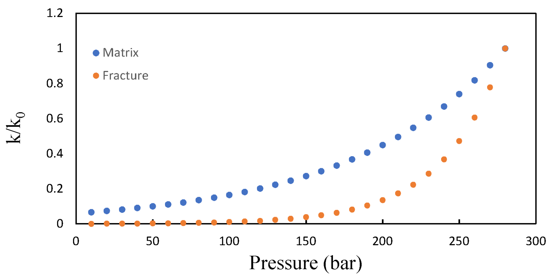
2.2. Threshold Pressure Gradient and Stress Sensitivity

In tight oil reservoirs, due to the porosity of the formation being extremely low, the fluid will not flow immediately under the action of force, and the minimum starting pressure needs to be overcome. Therefore, the flow of fluids in porous media is nonlinear seepage with a minimum threshold pressure gradient. The starting pressure gradient can affect the flow calculation of “matrix–matrix”, as well as the flow calculation of “matrix-crack” and “embedded crack-matrix”. So, it is necessary to consider the impact of the threshold pressure gradient on production capacity when conducting numerical simulations.
Previously, we have established component simulations. In the development process of low-permeability reservoirs, the flow of oil is affected by the starting pressure. However, many studies on the numerical simulation of CO2-HnP in tight oil reservoirs have not considered the starting pressure gradient [63,65,66]. This greatly reduces the accuracy of the simulation results. Therefore, the percolation law containing the starting pressure gradient was presented in the article. When considering the starting pressure gradient, the equation has strong nonlinearity. The equation below was introduced into the simulator to enable it to consider the influence of the starting pressure gradient [67].
When considering the starting pressure gradient, the expression for the flow rate of phase P can be written as follows:
q P , j i = ρ P k r P μ P T i j ( Φ P , j Φ P , i ) [ 1 λ ( | | Φ | | i j λ 0 ) + λ ]
where q represents the flow rate, P represents the gas phase or oil phase, λ represents the pressure gradient, λ0 represents the threshold value, Φ P , j and Φ P , i represent the pressure potential of grids j and i, respectively, | | Φ | | i j represents the pressure gradient between grids i and j, krP represents the relative permeability, and μP represents the P phase viscosity.
We set an example to examine the impact of the starting pressure gradient on the formation pressure field and the cumulative oil production of the well. We selected a well in the formation and conducted a one-year depleted development, followed by CO2-HnP development. After four rounds of CO2-HnP cycles, a total of 5 years of production was achieved. We set two scenarios: one considering the starting pressure gradient, and the other not considering it. Comparing the numerical simulations of CO2-HnP with and without considering the threshold pressure gradient, the results of the pressure field changes after four rounds of huff-n-puff are shown in Figure 4. It can be seen that the variation in formation pressure when considering the threshold pressure gradient is relatively smaller than that when not considering it, after the same production time.
The COP curve is shown in Figure 5. It can be seen that, considering the impact of the starting pressure gradient, the cumulative oil production is significantly lower than that without considering it after production for 5 years. This suggests that the effect of the starting pressure gradient cannot be ignored in simulations.
Rock stress sensitivity is another important factor affecting the development effectiveness of tight formations. For more accurate simulations, stress sensitivity is considered in the CO2-HnP model. Using the stress-related permeability correlation model, the production decline caused by the change in permeability in tight reservoirs can be simulated. In this article, we assume that the porosity does not vary with stress. The expression for stress-related permeability can be written as follows:
k = k 0 e A ( σ σ 0 )
where σ’ represents the effective stress, A represents the experimental coefficient, and σ0 represents the initial state. The coefficient used is obtained experimentally. Figure 6 illustrates the stress-sensitivity curves for the fractures and matrix in the model.
Similarly, we can take a comparative example. Based on the previous example of starting pressure, one scenario considers stress sensitivity and the other does not consider it. We investigated the impact of rock stress sensitivity on the formation pressure field and cumulative oil production of wells in two scenarios. Figure 7 shows the effect of stress sensitivity on the formation pressure field after a one-year depletion development, four cycles of CO2-HnP development, and a total of five years of production. Figure 7a shows the pressure field distribution without considering stress sensitivity. Figure 7b shows the distribution of the formation pressure field considering stress sensitivity. In Figure 7a, it can be seen that the color of the formation pressure field is darker. This indicates that the pressure field changes more significantly and that the range of changes is larger without considering stress sensitivity. Under the same production situation, the pressure field changes less without considering stress sensitivity, as shown in Figure 7b. There are obvious differences in the formation pressure field between the two situations.
The COP curve is shown in Figure 8. The blue line in Figure 8 represents the COP without considering stress sensitivity, while the orange line represents the COP when considering stress sensitivity in the model. We can see that the blue line is significantly higher than the orange line, and the value of the blue line is almost twice that of the orange line. This indicates that, without considering stress sensitivity, the cumulative oil production is abnormally high, which does not comply with the actual situation of unconventional reservoirs. So, when conducting numerical simulations, stress sensitivity is a factor that cannot be ignored.

3. Results and Discussion

Based on the reservoir model parameters and fluid characteristics set above, numerical simulations of CO2-HnP were conducted, and the effects of different CO2 injection conditions on the cumulative oil production were compared. The CO2-HnP process in a multistage-fracturing horizontal tight oil well consists of three main stages, as shown in Figure 1: CO2 injection, CO2 soaking, and production. In the compositional numerical simulation research, we conducted a series of simulations to determine the reasonable ranges and values of the uncertainty parameters that affect the CO2-HnP process, such as bottom-hole pressure, CO2 injection rate, CO2 injection time period, soaking time, and the number of cycles of CO2-HnP. Only one variable was changed at a time, while the other parameters remained unchanged. When comparing the results, the cumulative oil production was used as the measurement standard.
Here, we briefly describe the entire the CO2-HnP process in the basic case. Initially, as a production well, the horizontal well produces through depletion development for one year, and then it is switched to an injection well that injects CO2 at a rate of 50,000 cubic meters per day and maintains a bottom-hole pressure of 100 bar. After 30 days of CO2 injection, the well is shut down and kept soaking for another 30 days. After 30 days of soaking, the well is converted to a production well to resume production. This is one cycle of the CO2-HnP process. Each cycle lasts for 360 days, with one cycle ending and the other cycle starting. In this simulation study, the well was developed for a total of five years. The well experienced four cycles after one year of primary depletion development during the total production time.

3.1. Sensitivity Parameter Analysis for CO2 Huff-n-Puff

3.1.1. Effect of Bottom-Hole Pressure

In order to find a suitable bottom-hole pressure, numerical simulation calculations were carried out for six bottom-hole pressure values of 200 bar, 180 bar, 150 bar, 100 bar, 80 bar, and 75 bar, while keeping the other huff-n-puff parameters the same as in the basic case mentioned above. The bottom-hole pressure optimization plan is listed in Table 4. Simulation results for the effect of bottom-hole pressure on cumulative oil production are shown in Figure 9. The cumulative oil production is abbreviated as COP and the bottom-hole pressure is abbreviated as BHP in the following text.
Figure 9 is a histogram of cumulative oil production (COP) and bottom-hole pressure (BHP). The higher the blue bar in the graph, the higher the COP. From Figure 9, it can be seen that as the BHP decreases, the COP gradually increases. The results indicate that BHP has a significant influence on the COP. The lower the bottom-hole pressure, the higher the cumulative oil production. However, when the BHP drops to 100 bar, the increase in COP is not significant. That is, the BHP has an optimal value. This is because the lower the BHP, the greater the pressure gradient between the bottom hole and the formation. The greater the displacement energy in the formation, the higher the cumulative production of the well. However, when the BHP drops to a certain value, due to the stress sensitivity of the rock, the porosity and permeability of the rock decrease, making it difficult for oil to flow from the formation into the wellbore, resulting in a slower increase in well production. Because the increase in COP is already very small when the BHP reaches 100 bar, and the growth rate of COP essentially does not change, it is necessary to avoid excessive development of the formation due to low BHP, leading to a decrease in the reservoir’s porosity and permeability, while also obtaining the best cumulative oil production. Therefore, 100 bar is the optimal value. In the following case, the BHP value was set to 100 bar in order to obtain the most efficient COP.

3.1.2. Effect of CO2 Injection Rate

In order to find the best CO2 injection rate, numerical simulation calculations were carried out for four injection rates: 40,000 cubic meters per day, 50,000 cubic meters per day, 60,000 cubic meters per day, and 100,000 cubic meters per day, while maintaining the total injection volume of 600,000 cubic meters for each cycle and keeping the other huff-n-puff parameters constant. The parameters of the CO2 injection rate optimization scheme are shown in Table 5. Figure 10 shows the effect of the injection rate on COP.
In this case, we kept the total CO2 injection volume constant and chose different CO2 injection rates to simulate. When the CO2 injection rate was high, the corresponding injection time would decrease. We tried to find the optimal combination of injection rate and injection time through multiple scenario simulations. As shown in Figure 10, when the total gas injection volume remained unchanged, as the CO2 injection rate increased, the COP first increased and then gradually decreased, reaching a maximum value when the CO2 injection rate reached 50,000 cubic meters per day. This may be because the initial injection of CO2 takes a relatively long time and CO2 undergoes sufficient exchange with the original oil in the formation under the CO2 diffusion effect, resulting in more crude oil flowing into the well. However, when the injection rate increases to a certain value and the total injection amount is constant, the injection time becomes shorter, and CO2 does not have sufficient opportunities to be effectively replaced with crude oil. In the following simulation, we set the CO2 injection rate to 50,000 cubic meters per day.

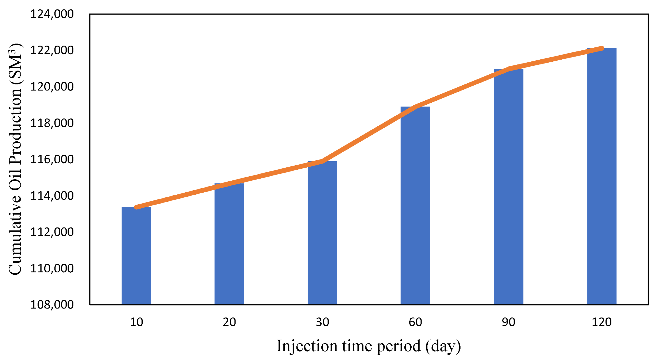
3.1.3. Effect of Injection Time

In order to find the optimal CO2 injection time period, we set the CO2 injection time period as 10 days, 20 days, 30 days, 60 days, 90 days, and 120 days, while keeping the other huff-n-puff parameters constant. That is, in each simulation case, the injection rate was set to the same 50000 cubic meters per day, the same soaking time, the same production time, and the same number of cycles, with the only difference being the injection time. The parameters of the CO2 injection time optimization scheme are shown in Table 6. Figure 11 shows the simulation results of the effect of the injection time period on COP.
In Figure 11, the blue bar represents the COP, while the orange line represents the trend of COP growth. The higher the blue bar, the higher the COP; the larger the slope of the orange line, the higher the COP growth; and the smaller the slope, the slower the COP growth. The injection time ranged from 10 days to 30 days, with a slow increase in cumulative production; from 30 days to 90 days, the COP increased rapidly, but from 90 days to 120 days, the growth rate of COP slowed down and gradually stabilized in the region. The results indicate that COP gradually increases with the extension of the injection time period. However, the COP growth rate slowed down from 3 months to 4 months. After 4 months of injection, the growth effect of COP was no longer significant. Therefore, there is a reasonable range of injection time. Due to the short duration of this simulation, in the following simulation cases, we will take an injection time of 20 days per cycle.

3.1.4. Effect of Soaking Time

The soaking time directly impacts the utilization rate of the injected CO2 during the huff-n-puff process. Based on the previously optimized injection rate and injection time, we optimized the soaking time of the well. Six different soaking times were set: 10 days, 15 days, 20 days, 30 days, 35 days, and 40 days. The injection rate was set to 50,000 cubic meters per day, the injection time was set to 20 days, the production time was set to 360 days, and there were four cycles. The other parameters remain unchanged. Table 7 shows the parameters of the soaking time optimization scheme. Figure 12 shows the effect of soaking time on cumulative oil production (COP).
Similarly, the blue bars in Figure 12 represent cumulative oil production (COP), while the orange line represents the trend of cumulative oil production (COP) growth. It can be seen from Figure 12 that when the soaking time ranges from 10 days to 20 days, the COP slowly increases. When the soaking time increases from 20 days to 35 days, the COP increases rapidly, but when the soaking time is greater than 35 days, the COP essentially does not increase. This implies that as the soaking time increases, the COP also gradually increases, but when the soaking time extends to a certain value, the COP growth is not significant. So, there is an optimal soaking time for the well. The optimal final soaking time is 35 days. In the following simulation case, the soak time was set to 35 days per cycle.

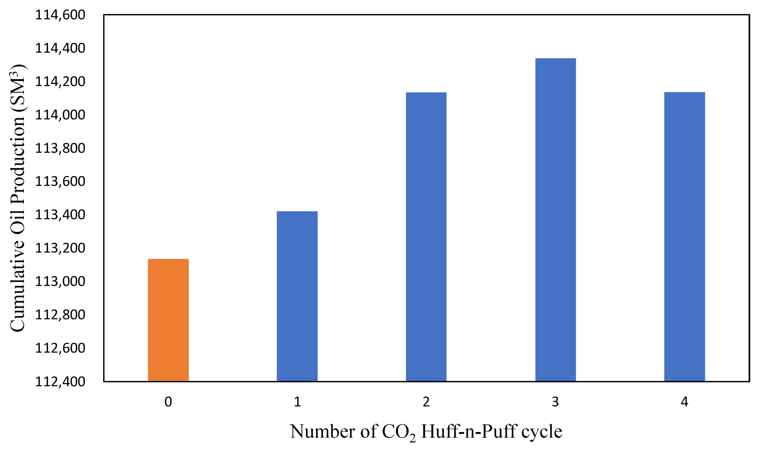
3.1.5. Effect of the Number of CO2 Huff-n-Puff Cycles

In order to find a suitable number of CO2-HnP cycles, the number of cycles was set to 1, 2, 3, and 4, while the other HnP parameters were kept constant. In order to compare the impact of the number of CO2-HnP cycles on the well’s production efficiency, a simulation case of depleted development without cycles was carried out. The injection rate was set to 50,000 cubic meters per day, the injection time was set to 20 days, the soaking time was set to 35 days, and the production time was set to 360 days. All of the other parameters remained unchanged, with only the number of cycles changing. Table 8 shows the parameter list for the number of CO2-HnP cycles optimization scheme in simulations, while Figure 13 shows the effect of the number of CO2-HnP cycles on COP.
In Figure 13, the orange bars represent depleted development without external energy supplementation, while the blue bars represent different numbers of CO2-HnP cycles. From Figure 13, it can be seen that all of the blue bars are significantly higher than the orange bar, which indicates that CO2-HnP can indeed significantly increase oil production and improve oil recovery. Next, we take a look at the impact of the number of cycles on the COP. After increasing the number of cycles from one to three, the COP gradually increases. After three cycles, the COP begins to decrease. At the time of three cycles of huff-n-puff, the COP reaches its maximum. The optimal final number of CO2-HnP cycles is three.

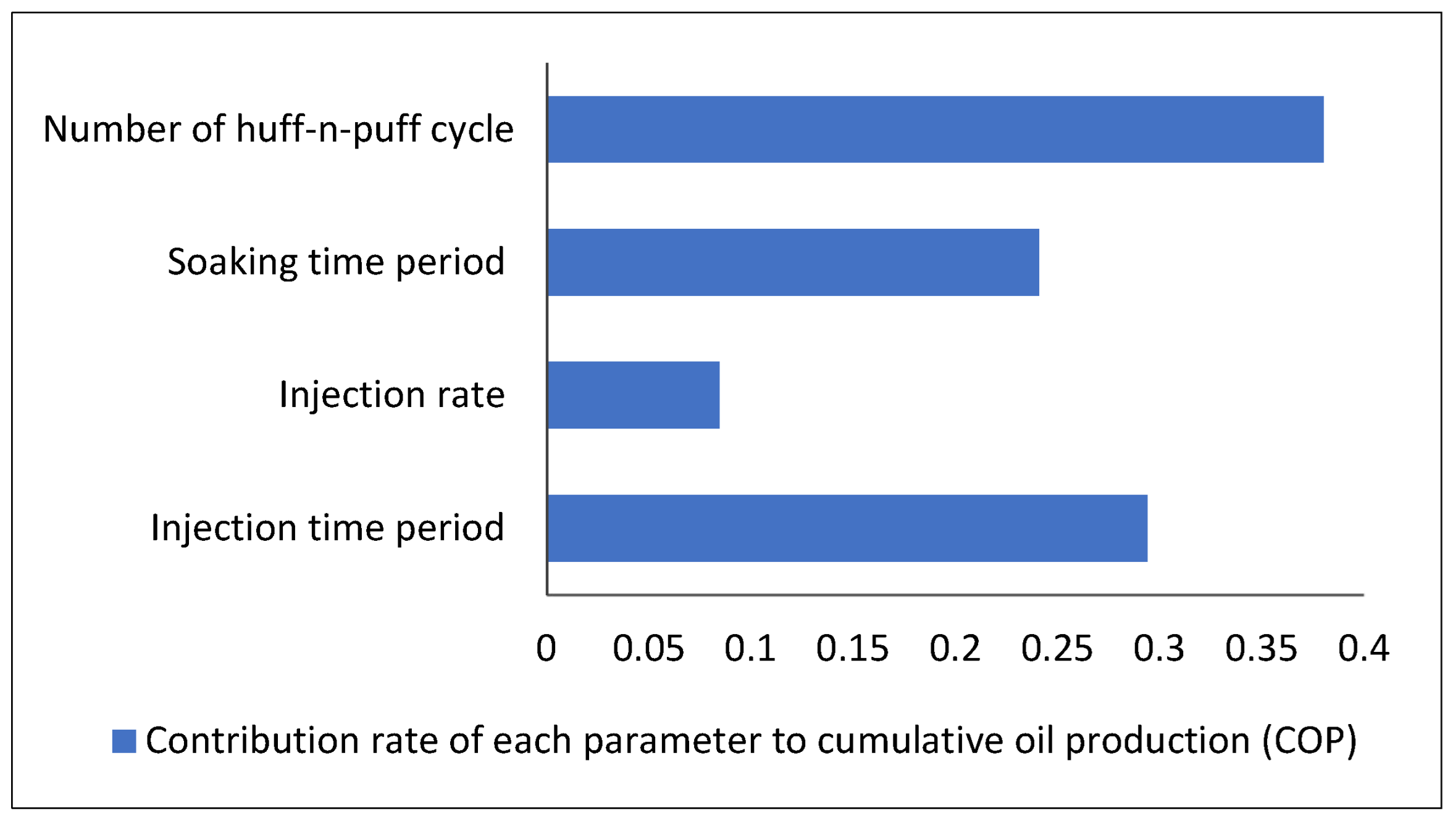
3.1.6. Comprehensive Analysis of Multiple Factors Affecting COP

In order to understand and estimate the effects of the above sensitivity parameters on COP, we need to analyze the weight of each parameter’s impact on the COP. After numerical simulation, the COP under each variable parameter can be obtained. The decision tree method was applied to calculate the contribution of each parameter to COP, and then the impact degree values calculated by machine learning were drawn into bar charts (Figure 14) and pie charts (Figure 15). Figure 14 and Figure 15 represent the contribution of all sensitivity parameters to COP. In Figure 14, the blue bars represent the percentage of impact of the parameters on COP. The longer the blue bar, the greater the impact of this parameter on COP. From Figure 14, it can be seen that the number of cycles has the greatest impact on COP, followed by the injection time and soak time, while the injection rate has the smallest impact on COP. Similarly, in Figure 15, the size of the sector and the percentage in the sector represent the degree of influence of the parameters on COP. The larger the sector, the greater the impact of the parameter on COP. The larger the percentage value, the greater the impact of the parameter on COP. From Figure 15, it can be seen that the degree of influence of the number of cycles accounts for 38.04%, the degree of influence of injection time accounts for 29.41%, the soaking time accounts for 24.10%, and the injection rate accounts for 8.45%. The number of cycles contributes the most to COP, followed by the injection time and soak time, with the injection rate contributing the least.

4. Conclusions

In this study, a component numerical simulation model based on discrete fracture model technology was established to simulate the CO2-HnP process of multistage fractured horizontal wells in tight reservoirs with complex fractures. This model can serve as a universal framework for CO2-HnP in unconventional fractured reservoirs. Taking into account the starting pressure gradient and stress sensitivity, a series of sensitive parameters affecting CO2-HnP efficiency were simulated, and their impacts on cumulative production were analyzed. The following conclusions can be drawn:
(1)
The latest embedded discrete fracture technology (EDFM) was applied in the model, making the simulation of CO2 huff-n-puff in complex fractured reservoirs faster and more efficient.
(2)
The starting pressure gradient and rock stress sensitivity factors greatly affect the pressure field of tight reservoirs and the cumulative production of multistage-fracturing horizontal wells. The rock stress sensitivity influences the reservoir’s permeability and porosity, and the starting pressure gradient can interfere with the flow calculation of “matrix–matrix”, as well as the flow calculation of “matrix-fracture” and “embedded fracture–matrix”, which cannot be ignored in component numerical simulations.
(3)
In CO2 huff-n-puff simulations, production parameters such as injection rate, injection time, soak time, and the number of cycles all have an impact on COP. The degree of influence of the number of cycle accounts for 38.04%, the injection time accounts for 29.41%, the soaking time accounts for 24.10%, and the injection rate accounts for 8.45%. So, the number of cycles contributes the most to COP, followed by injection time and soak time, with the injection rate contributing the least. The injection rate and the number of cycles both have optimal values, while the injection time and soak time tend to have less significant effects on the growth of COP over time. Based on the results of our numerical simulations, the plan of injecting CO2 at a daily injection rate of 50,000 cubic meters for 20 days, soaking for 35 days, circulating for three rounds, and producing for 5 years can achieve the highest cumulative production.
(4)
This study provides a universal and more efficient numerical simulation method for CO2 huff-n-puff in multistage-fracturing horizontal wells of complex fractured tight oil reservoirs. The innovation of this study is the integration of nonlinear seepage with the starting pressure gradient, stress sensitivity, and EDFM technology.

Author Contributions

Conceptualization, J.Z., L.W. and X.C.; methodology, Z.W. and L.W.; validation, S.J.; formal analysis, Z.C.; investigation, F.S.; resources, T.J.; data curation, X.C.; writing—original draft preparation, J.Z. and X.C.; writing—review and editing, J.Z., Z.W. and X.C.; visualization, Z.C.; supervision, F.S.; project administration, T.J.; funding acquisition, Z.W. All authors have read and agreed to the published version of the manuscript.

Funding

This research received no external funding.

Data Availability Statement

Data are contained within the article.

Acknowledgments

We thank Energy Innovation Software for providing technical support. The authors also thank the journal editor and reviewers for their valuable comments and suggestions.

Conflicts of Interest

Author Jiayu Zheng, Tianhao Jiang, Zhengpan Cui and Fangxin Song were employed by the company PetroChina Changqing Oilfield Company. The remaining authors declare that the re-search was conducted in the absence of any commercial or financial relationships that could be construed as a potential conflict of interest.

References

  1. Weixiang, C.; Chunpeng, W. Carbon capture, utilization and storage (CCUS) in tight oil reservoir. In Proceedings of the Abu Dhabi International Petroleum Exhibition and Conference, Abu Dhabi, United Arab Emirates, 2 October 2023. [Google Scholar]
  2. Joslin, K.; Ghedan, S.G.; Abraham, A.M.; Pathak, V. EOR in tight reservoirs, technical and economical feasibility. In Proceedings of the SPE Unconventional Resources Conference, Calgary, AB, Canada, 15 February 2017. [Google Scholar]
  3. Todd, H.B.; Evans, J.G. Improved Oil Recovery IOR Pilot Projects in the Bakken Formation. In Proceedings of the SPE Low Perm Symposium, Denver, CO, USA, 5 May 2016. [Google Scholar]
  4. Kang, Y.; Tian, J.; Luo, P.; Liu, X. Technical bottlenecks and development straegies of enhancing recovery for tight oil reserviors. Acta Pet. Sin. 2020, 41, 468–479. [Google Scholar]
  5. Gale, J.F.W.; Laubach, S.E.; Olson, J.E.; Eichhubl, P.; Fall, A. Natural fractures in shale: A review and new observations. AAPG Bull. 2014, 98, 2165–2216. [Google Scholar] [CrossRef]
  6. Hu, T.; Pang, X.; Wang, X.; Pang, H.; Liu, Y.; Wang, Y.; Tang, L.; Chen, L.; Pan, Z.; Xu, J.; et al. Tight oil play characterisation: The lower-middle Permian Lucaogou Formation in the Jimusar Sag, Junggar Basin, Northwest China. Aust. J. Earth Sci. 2016, 63, 349–365. [Google Scholar] [CrossRef]
  7. Fisher, M.K.; Wright, C.A.; Davidson, B.M.; Goodwin, A.K.; Fielder, E.O.; Buckler, W.S.; Steinsberger, N.P. Integrating fracture mapping technologies to optimize stimulations in the Barnett Shale. In Proceedings of the SPE Annual Technical Conference and Exhibition, San Antonio, TX, USA, 29 September 2002. [Google Scholar]
  8. Xu, Y.; Cavalcante, J.S.A.; Yu, W.; Sepehrnoori, K. Discrete-fracture modeling of complex hydraulic-fracture geometries in reservoir simulators. SPE Reserv. Eval. Eng. 2017, 20, 403–422. [Google Scholar] [CrossRef]
  9. Moinfar, A.; Varavei, A.; Sepehrnoori, K.; Johns, R.T. Development of a novel and computationally-efficient discrete-fracture model to study ior processes in naturally fractured reservoirs. In Proceedings of the SPE Improved Oil Recovery Symposium, Tulsa, OK, USA, 14–18 April 2012. [Google Scholar]
  10. Barenblatt, G.I.; Zheltov, I.P.; Kochina, I. Basic concepts in the theory of seepage of homogeneous liquids in fissured rocks [strata]. J. Appl. Math. Mech. 1960, 24, 1286–1303. [Google Scholar] [CrossRef]
  11. Warren, J.E.; Root, P.J. The behavior of naturally fractured reservoirs. SPE J. 1963, 3, 245–255. [Google Scholar] [CrossRef]
  12. Dean, R.; Lo, L. Development of a natural fracture simulator and examples of its use. In Proceedings of the International Meeting on Petroleum Engineering, Beijing, China, 17–20 March 1986. [Google Scholar]
  13. Odling, N.; Gillespie, P.; Bourgine, B.; Castaing, C.; Chiles, J.; Christensen, N.; Fillion, E.; Genter, A.; Olsen, C.; Thrane, L. Variations in fracture system geometry and their implications for fluid flow in fractures hydrocarbon reservoirs. Petrol. Geosci. 1999, 5, 373–384. [Google Scholar] [CrossRef]
  14. Kazemi, H.; Merrill Jr, L.; Porterfield, K.; Zeman, P. Numerical simulation of water-oil flow in naturally fractured reservoirs. SPE J. 1976, 16, 317–326. [Google Scholar] [CrossRef]
  15. Rossen, R. Simulation of naturally fractured reservoirs with semi-implicit source terms. SPE J. 1977, 17, 201–210. [Google Scholar] [CrossRef]
  16. Blaskovich, F.; Cain, G.; Sonier, F.; Waldren, D.; Webb, S. A multicomponent isothermal system for efficient reservoir simulation. In Proceedings of the SPE Middle East Oil and Gas Show and Conference, Manama, Bahrain, 14 March 1983; p. SPE–11480-MS. [Google Scholar]
  17. Hill, A.; Thomas, G. A new approach for simulating complex fractured reservoirs. In Proceedings of the SPE Middle East Oil and Gas Show and Conference, Manama, Bahrain, 11–14 March 1985. [Google Scholar]
  18. Saidi, A. Simulation of naturally fractured reservoirs. In Proceedings of the SPE Reservoir Simulation Conference, San Francisco, CA, USA, 26–28 February 1983. [Google Scholar]
  19. Gillespie, P.; Howard, C.; Walsh, J.; Watterson, J. Measurement and characterisation of spatial distributions of fractures. Tectonophysics 1993, 226, 113–141. [Google Scholar] [CrossRef]
  20. Moinfar, A.; Narr, W.; Hui, M.-H.; Mallison, B.; Lee, S.H. Comparison of discrete-fracture and dual-permeability models for multiphase flow in naturally fractured reservoirs. In Proceedings of the SPE Reservoir Simulation Conference, Abu Dhabi, UAE, 9–11 October 2011. [Google Scholar]
  21. Al-Hinai, O.; Singh, G.; Pencheva, G.; Almani, T.; Wheeler, M.F. Modeling multiphase flow with nonplanar fractures. In Proceedings of the SPE Reservoir Simulation Symposium, The Woodlands, TX, USA, 18 February 2013. [Google Scholar]
  22. Hui, M.-H.R.; Mallison, B.; Heidary-Fyrozjaee, M.; Narr, W. The upscaling of discrete fracture models for faster, coarse-scale simulations of IOR and EOR processes for fractured reservoirs. In Proceedings of the SPE Annual Technical Conference and Exhibition, New Orleans, LA, USA, 1 October 2013. [Google Scholar]
  23. Karimi-Fard, M.; Durlofsky, L.J.; Aziz, K. An efficient discrete-fracture model applicable for general-purpose reservoir simulators. SPE J. 2004, 9, 227–236. [Google Scholar] [CrossRef]
  24. Monteagudo, J.E.P.; Firoozabadi, A. Control-volume method for numerical simulation of two-phase immiscible flow in two- and three-dimensional discrete-fractured media. Water Resour. Res. 2004, 40, W07405. [Google Scholar] [CrossRef]
  25. Noorishad, J.; Mehran, M. An upstream finite element method for solution of transient transport equation in fractured porous media. Water Resour. Res. 1982, 18, 588–596. [Google Scholar] [CrossRef]
  26. Olorode, O.M.M.; Freeman, C.M.M.; Moridis, G.J.J.; Blasingame, T.A.A. High-resolution numerical modeling of complex and irregular fracture patterns in shale-gas reservoirs and tight gas reservoirs. SPE Reserv. Eval. Eng. 2013, 16, 443–455. [Google Scholar] [CrossRef]
  27. Sandve, T.H.; Berre, I.; Nordbotten, J.M. An efficient multi-point flux approximation method for Discrete Fracture–Matrix simulations. J. Comput. Phys. 2012, 231, 3784–3800. [Google Scholar] [CrossRef]
  28. Li, L.; Lee, S.H. Efficient field-scale simulation of black oil in a naturally fractured reservoir through discrete fracture networks and homogenized media. SPE Reserv. Eval. Eng. 2008, 11, 750–758. [Google Scholar] [CrossRef]
  29. Qin, J.; Xu, Y.; Tang, Y.; Liang, R.; Zhong, Q.; Yu, W.; Sepehrnoori, K. Impact of complex fracture networks on rate transient behavior of wells in unconventional reservoirs based on embedded discrete fracture model. J. Energy Resour. Technol. 2021, 144, 083007. [Google Scholar] [CrossRef]
  30. Shakiba, M.; Sepehrnoori, K. Using embedded discrete fracture model (EDFM) and microseismic monitoring data to characterize the complex hydraulic fracture networks. In Proceedings of the SPE Annual Technical Conference and Exhibition, Houston, TX, USA, 30 September 2015. [Google Scholar]
  31. Lee, S.H.; Jensen, C.L.; Lough, M.F. Efficient finite-difference model for flow in a reservoir with multiple length-scale fractures. SPE J. 2000, 5, 268–275. [Google Scholar] [CrossRef]
  32. Li, J.; Tang, H.; Zhang, Y.; Li, X. An adaptive grid refinement method for flow-based embedded discrete fracture models. In Proceedings of the SPE Reservoir Simulation Conference, Galveston, TX, USA, 21 March 2023. [Google Scholar]
  33. Fiallos, M.X.; Yu, W.; Ganjdanesh, R.; Kerr, E.; Sepehrnoori, K.; Miao, J.; Ambrose, R. Modeling interwell interference due to complex fracture hits in eagle ford using EDFM. In Proceedings of the International Petroleum Technology Conference, Beijing, China, 26 March 2019. [Google Scholar]
  34. Yu, W.; Lashgari, H.R.; Wu, K.; Sepehrnoori, K. CO2 injection for enhanced oil recovery in Bakken tight oil reservoirs. Fuel 2015, 159, 354–363. [Google Scholar] [CrossRef]
  35. Askarova, A.; Turakhanov, A.; Mukhina, E.; Cheremisin, A.; Cheremisin, A. Unconventional reservoirs: Methodological approaches for thermal EOR simulation. In Proceedings of the SPE/AAPG/SEG Unconventional Resources Technology Conference, Virtual, 22 July 2020. [Google Scholar]
  36. Khakimova, L.; Askarova, A.; Popov, E.; Moore, R.G.; Solovyev, A.; Simakov, Y.; Afanasiev, I.; Belgrave, J.; Cheremisin, A. High-pressure air injection laboratory-scale numerical models of oxidation experiments for Kirsanovskoye oil field. J. Pet. Sci. Eng. 2020, 188, 106796. [Google Scholar] [CrossRef]
  37. Lee, K.; Moridis, G.J.; Ehlig-Economides, C.A. A Comprehensive simulation model of kerogen pyrolysis for the in-situ upgrading of oil shales. SPE J. 2016, 21, 1612–1630. [Google Scholar] [CrossRef]
  38. Liu, J.; Chen, H.; Zhao, S.; Pan, P.; Wu, L.; Xu, G. Evaluation and improvements on the flexibility and economic performance of a thermal power plant while applying carbon capture, utilization & storage. Energy Conv. Manag. 2023, 290, 117219. [Google Scholar]
  39. Mukhina, E.; Askarova, A.; Kalacheva, D.; Leushina, E.; Kozlova, E.; Cheremisin, A.; Morozov, N.; Dvoretskaya, E.; Demo, V.; Cheremisin, A. Hydrocarbon saturation for an unconventional reservoir in details. In Proceedings of the SPE Russian Petroleum Technology Conference, Moscow, Russia, 24 October 2019. [Google Scholar]
  40. He, T.; Li, W.; Lu, S.; Yang, E.; Jing, T.; Ying, J.; Zhu, P.; Wang, X.; Pan, W.; Zhang, B.; et al. Quantitatively unmixing method for complex mixed oil based on its fractions carbon isotopes: A case from the Tarim Basin, NW China. Petrol. Sci. 2023, 20, 102–113. [Google Scholar] [CrossRef]
  41. Liu, S.; Sahni, V.; Tan, J.; Beckett, D.; Vo, T. Laboratory investigation of eor techniques for organic rich shales in the permian basin. In Proceedings of the SPE/AAPG/SEG Unconventional Resources Technology Conference, Houston, TX, USA, 25 July 2018. [Google Scholar]
  42. Sennaoui, B.; Pu, H.; Malki, M.L.; Afari, A.S.; Larbi, A. Reservoir simulation study and optimizations of CO2 huff-n-puff mechanisms in three forks formation. In Proceedings of the International Geomechanics Symposium, Abu Dhabi, UAE, 7 November 2022. [Google Scholar]
  43. Erofeev, A.A.; Mitrushkin, D.A.; Meretin, A.S.; Pachezhertsev, A.A.; Karpov, I.A.; Demo, V.O. Simulation of thermal recovery methods for development of the bazhenov formation. In Proceedings of the SPE Russian Petroleum Technology Conference and Exhibition, Moscow, Russia, 24 October 2016. [Google Scholar]
  44. Kang, Z.; Zhao, Y.; Yang, D. Review of oil shale in-situ conversion technology. Appl. Energy 2020, 269, 115121. [Google Scholar] [CrossRef]
  45. Hassan, A.M.; Ayoub, M.; Eissa, M.; Al-Shalabi, E.W.; Almansour, A.; Alquraishi, A. Foamability and foam stability screening for smart water assisted foam flooding: A new hybrid eor method. In Proceedings of the International Petroleum Technology Conference, Riyadh, Saudi Arabia, 22 February 2022. [Google Scholar]
  46. Downey, R.; Venepalli, K.; Erdle, J.; Whitelock, M. A superior shale oil eor method for the permian basin. In Proceedings of the SPE Annual Technical Conference and Exhibition, Dubai, United Arab Emirates, 22 September 2021. [Google Scholar]
  47. Rezaei Koochi, M.; Mehrabi-Kalajahi, S.; Varfolomeev, M.A. Thermo-Gas-Chemical stimulation as a revolutionary ior-eor method by the in-situ generation of hot nitrogen and acid. In Proceedings of the SPE Annual Technical Conference and Exhibition, Dubai, United Arab Emirates, 22 September 2021. [Google Scholar]
  48. Holm, L.; Josendal, V. Mechanisms of oil displacement by carbon dioxide. J. Pet. Technol. 1974, 26, 1427–1438. [Google Scholar] [CrossRef]
  49. Holm, W.L. Evolution of the carbon dioxide flooding processes. J. Pet. Technol. 1987, 39, 1337–1342. [Google Scholar] [CrossRef]
  50. Strack, K.; Barajas-Olalde, C.; Davydycheva, S.; Martinez, Y.; Paembonan, A. CCUS plume monitoring: Verifying surface csem measurements to log scale. In Proceedings of the SPWLA 64th Annual Logging Symposium, Lake Conroe, TX, USA, 13 June 2023. [Google Scholar]
  51. Paskvan, F.; Paine, H.; Resler, C.; Sheets, B.; McGuire, T.; Connors, K.; Tempel, E. Alaska CCUS workgroup and a roadmap to commercial deployment. In Proceedings of the SPE Western Regional Meeting, Anchorage, AK, USA, 24 May 2023. [Google Scholar]
  52. Bao, X.; Fragoso, A.; Aguilera, R. CCUS and comparison of oil recovery by huff n puff gas injection using methane, carbon dioxide, hydrogen and rich gas in shale oil reservoirs. In Proceedings of the SPE Canadian Energy Technology Conference and Exhibition, Calgary, AB, Canada, 16 March 2023. [Google Scholar]
  53. Halinda, D.; Zariat, A.A.; Muraza, O.; Marteighianti, M.; Setyawan, W.; Haribowo, A.; Rajab, M.; Firmansyah, M.; Hasan, I.; Nurlia, D.; et al. CO2 huff and puff injection operation overview in jatibarang field lessons learned from a successful case study in mature oil field. In Proceedings of the Abu Dhabi International Petroleum Exhibition and Conference, Abu Dhabi, United Arab Emirates, 2 October 2023. [Google Scholar]
  54. Zhao, J.; Jin, L.; Azzolina, N.A.; Wan, X.; Yu, X.; Sorensen, J.A.; Kurz, B.A.; Bosshart, N.W.; Smith, S.A.; Wu, C.; et al. Investigating enhanced oil recovery in unconventional reservoirs based on field case review, laboratory, and simulation studies. Energ. Fuel 2022, 36, 14771–14788. [Google Scholar] [CrossRef]
  55. Sun, Y.; Li, S.; Sun, R.; Liu, X.; Pu, H.; Zhao, J. Study of CO2 enhancing shale gas recovery based on competitive adsorption theory. ACS Omega 2020, 5, 23429–23436. [Google Scholar] [CrossRef]
  56. Wang, T.; Xu, B.; Chen, Y.T.; Wang, J. Mechanism and main control factors of CO2 huff and puff to enhance oil recovery in chang 7 shale oil reservoir of Ordos Basin. Processes 2023, 11, 2726. [Google Scholar] [CrossRef]
  57. Zhang, S.; Jia, B.; Zhao, J.; Pu, H. A diffuse layer model for hydrocarbon mass transfer between pores and organic matter for supercritical CO2 injection and sequestration in shale. Chem. Eng. J. 2021, 406, 126746. [Google Scholar] [CrossRef]
  58. Li, L.; Su, Y.; Sheng, J.J.; Hao, Y.; Wang, W.; Lv, Y.; Zhao, Q.; Wang, H. Experimental and numerical study on CO2 sweep volume during CO2 huff-n-puff enhanced oil recovery process in shale oil reservoirs. Energ. Fuel 2019, 33, 4017–4032. [Google Scholar] [CrossRef]
  59. El Morsy, M.; Ali, S.; Giddins, M.A.; Fitch, P. CO2 injection for improved recovery in tight gas condensate reservoirs. In Proceedings of the SPE Asia Pacific Oil & Gas Conference and Exhibition, Virtual, 19 November 2020. [Google Scholar]
  60. Seteyeobot, I.; Jamiolahmady, M.; Doryanidaryuni, H.; Molokwu, V. A Coreflood simulation study of a systematic CO2 huff-n-puff injection for storage and enhanced gas condensate recovery. In Proceedings of the SPE Annual Technical Conference and Exhibition, Houston, TX, USA, 5 October 2022. [Google Scholar]
  61. Zhang, Y.; Yu, W.; Li, Z.; Sepehrnoori, K. Simulation study of factors affecting CO2 Huff-n-Puff process in tight oil reservoirs. J. Pet. Sci. Eng. 2018, 163, 264–269. [Google Scholar] [CrossRef]
  62. Zhao, J.; Wang, P.; Yang, H.; Tang, F.; Ju, Y.; Jia, Y. Experimental investigation of the CO2 huff and puff effect in low-permeability sandstones with NMR. ACS Omega 2021, 6, 15601–15607. [Google Scholar] [CrossRef] [PubMed]
  63. Lei, Z.; Wu, S.; Yu, T.; Ping, Y.; Qin, H.; Yuan, J.; Zhu, Z.; Su, H. Simulation and optimization of CO2 huff-n-puff processes in tight oil reservoir: A case study of Chang-7 tight oil reservoirs in Ordos Basin. In Proceedings of the SPE Asia Pacific Oil and Gas Conference and Exhibition, Jakarta, Indonesia, 24 October 2018. [Google Scholar]
  64. Alfarge, D.; Wei, M.; Bai, B. Chapter 3—Comparative analysis between CO2-EOR mechanisms in conventional reservoirs versus shale and tight reservoirs. In Developments in Petroleum Science; Elsevier: Amsterdam, The Netherlands, 2020; Volume 67, pp. 45–63. [Google Scholar]
  65. Cao, M.; Wu, X.; An, Y.; Zuo, Y.; Wang, R.; Li, P. Numerical simulation and performance evaluation of CO2 huff-n-puff processes in unconventional oil reservoirs. In Proceedings of the Carbon Management Technology Conference, Houston, TX, USA, 17 July 2017. [Google Scholar]
  66. Kurtoglu, B.; Sorensen, J.A.; Braunberger, J.; Smith, S.; Kazemi, H. Geologic characterization of a bakken reservoir for potential CO2 EOR. In Proceedings of the SPE/AAPG/SEG Unconventional Resources Technology Conference, Denver, CO, USA, 12–14 August 2013. [Google Scholar]
  67. Li, X.; Zhang, D.; Li, S. A multi-continuum multiple flow mechanism simulator for unconventional oil and gas recovery. J. Nat. Gas. Sci. Eng. 2015, 26, 652–669. [Google Scholar] [CrossRef]
Figure 1. The CO2-HnP process in a multistage horizontal well with hydraulic fractures and natural fractures: (a) CO2 injection; (b) CO2 soaking; (c) production.
Energies 16 07538 g001
Figure 2. Three-dimensional (3D) reservoir model with embedded discrete fractures in the article.
Energies 16 07538 g002
Figure 3. Relative permeability curves: (a) Water/oil relative permeability curve. (b) Gas/oil relative permeability curve.
Energies 16 07538 g003
Figure 4. Pressure field distribution: (a) Not considering the impact of the threshold pressure gradient. (b) Considering the impact of the threshold pressure gradient.
Energies 16 07538 g004
Figure 5. The impact of the threshold pressure gradient on cumulative oil production (COP).
Energies 16 07538 g005
Figure 6. Stress-sensitivity curves for the matrix and fractures.
Energies 16 07538 g006
Figure 7. Pressure field distribution: (a) Not considering the impact of stress sensitivity. (b) Considering the impact of stress sensitivity.
Energies 16 07538 g007
Figure 8. The impact of stress sensitivity on cumulative oil production (COP).
Energies 16 07538 g008
Figure 9. Effect of bottom-hole pressure (BHP) on cumulative oil production (COP).
Energies 16 07538 g009
Figure 10. Effect of injection rate on cumulative oil production (COP).
Energies 16 07538 g010
Figure 11. Effect of injection time period on cumulative oil production (COP).
Energies 16 07538 g011
Figure 12. Effect of soaking time on cumulative oil production (COP).
Energies 16 07538 g012
Figure 13. Effect of the number of CO2 huff-n-puff cycles on cumulative oil production (COP).
Energies 16 07538 g013
Figure 14. Degree of impact of each parameter affecting cumulative oil production (COP).
Energies 16 07538 g014
Figure 15. The pie graph of each parameter affecting cumulative oil production (COP).
Energies 16 07538 g015
Table 1. Basic parameters of the reservoir and fractures.
ParameterValueUnit
Model size (x × y × z)2000 × 1000 × 40m
Number of grid blocks (x × y × z)50 × 25 × 5
Reservoir permeability0.01mD
Reservoir porosity15%
Rock compressibility9.72 × 10−5bar−1
Reservoir thickness40m
Well length1200m
Fracture half-length150m
Fracture height40m
Fracture permeability2000mD
Table 2. Compositional data of the fluid components.
ComponentMolar
Fraction
Critical Pressure (Bar)Critical Temperature (K)Critical Volume (m3/kg⸱mol)Molecular
Weigh
Acentric
Factor
Parachor
Coefficient
CO20.017273.866304.70.09400066144.010.22578
N20.01433.944126.20.08999923628.0130.0441
C10.195846.042190.60.09800035216.0430.01377
C20.073648.839305.430.1479964530.070.0986108
C3–C50.130242.455369.80.1999974844.0970.1524150.3
C60.260630.104507.50.35099954840.299271
C70.2329.3845480.39200317960.3312.5
C80.078628.7975750.432999291070.312351.5
Table 3. Binary interaction parameters for the components.
ComponentCO2N2C1C2C3–C5C6C7C8
CO20−0.0120.10.10.10.10.10.1
N2−0.01200.10.10.10.10.10.1
C10.10.10000.02790.033080.0363
C20.10.10000.010.010.01
C3–C50.10.10000.010.010.01
C60.10.10.02790.010.01000
C70.10.10.033080.010.01000
C80.10.10.03630.010.01000
Table 4. Bottom-hole pressure (BHP) optimization plan.
Bottom-Hole Pressure (Bar)Injection Rate (m3/day)Injection Time Period (Day)Soaking Time Period (Day)
20050,0003030
18050,0003030
15050,0003030
10050,0003030
8050,0003030
7550,0003030
Table 5. Injection rate optimization scheme.
Injection Rate (m3/day)Injection Time Period (Day)Soaking Time Period (Day)Number of CO2 Huff-n-Puff Cycles
40,00015304
50,00012304
60,00010304
100,0006304
Table 6. Injection time period optimization scheme.
Injection Rate (m3/day)Injection Time Period (Day)Soaking Time Period (Day)Number of Huff-n-Puff Cycles
50,00010304
50,00020304
50,00030304
50,00060304
50,00090304
50,000120304
Table 7. Soaking time optimization scheme.
Injection Rate (m3/day)Injection Time Period (Day)Soaking Time Period (Day)Number of Huff-n-Puff Cycles
50,00020104
50,00020154
50,00020204
50,00020304
50,00020354
50,00020404
Table 8. Number of CO2 huff-n-puff cycles optimization scheme.
Injection Rate (m3/day)Injection Time Period (Day)Soaking Time Period (Day)Number of Huff-n-Puff Cycles
50,00020350
50,00020351
50,00020352
50,00020353
50,00020354
Disclaimer/Publisher’s Note: The statements, opinions and data contained in all publications are solely those of the individual author(s) and contributor(s) and not of MDPI and/or the editor(s). MDPI and/or the editor(s) disclaim responsibility for any injury to people or property resulting from any ideas, methods, instructions or products referred to in the content.

