A Rigorous Explicit Expression for the Mutual Inductance of Two Co-Axial Thin-Wire Coil Antennas Placed above a Layered Ground

Abstract

This paper presents a quasi-analytical method that allows the derivation of a rigorous series-form representation for the mutual inductance of two co-axial coil antennas located above an arbitrarily layered earth structure. Starting from Biot–Savart law, which gives the integral representation for the primary vector potential generated by the source coil, the potential reflected by the layered ground is derived, and the resulting total vector potential is then integrated along the external circumference of the receiving coil to give the mutual inductance of the two antennas. The obtained representation for the flux is then evaluated analytically through the usage of the Gegenbauer addition theorem once an accurate, rational approximation is used in place of the factor of the integrand that exhibits branch cuts. It is shown how the resulting explicit solution exhibits the same degree of accuracy as purely numerical approaches like the finite-difference time-domain (FDTD) method and conventional numerical quadrature schemes, while it is less time-demanding than the latter methods.

1. Introduction

In recent decades, the problem of calculating the mutual inductance of two-coil antennas has arisen in several areas of science and technology related to energy production and consumption. Examples of areas of interest include wireless power transfer (WPT) [1,2], magnetic resonance imaging [3,4,5], radio remote sensing [6,7,8,9,10,11], and geophysical prospecting for the detection of shallow buried objects [12,13,14]. In general, the need to calculate the mutual inductance of two coils originates in all the situations where it is required to strengthen or to mitigate, depending on the application, the inductive coupling between pairs of coils included in 3-D geometric arrangements of conductors. For instance, a reduction of magnetic coupling is desired in applications where several coils are supposed to work together without interfering with one another. An excellent illustration of such applications is magnetic resonance imaging (MRI), which involves multiple receivers placed in the neighborhood of each other, with the scope to ensure the coverage of a prescribed area. In that case, minimization of inductive crosstalk among neighboring coils is always a prerequisite to achieving high signal-to-noise ratio images [3,4]. Conversely, inductive coupling enhancement is pursued in wireless power transfer (WPT) systems. Examples are the two-coil WPT devices used in the framework of wireless charging systems for battery electric vehicles (BEV). Here, electrical energy is transmitted from an emitter to a receiver via magnetic induction without resorting to wires and cables [15,16,17,18,19,20], and it is easily understood how the efficiency of the energy transfer is strictly related to the strength of the magnetic coupling.

In all the considered applications, the ability to accurately determine the mutual inductance of a couple of coils plays a fundamental role in gaining helpful knowledge about the coupling strength. A variety of analytical procedures have been presented over the years [21,22,23,24,25,26,27] which have addressed the problem of computing the mutual inductance of two coils. Unfortunately, the main drawback of these formulas resides in that they are tailored to the free-space case and cannot be applied in the presence of an earth structure, which would alter the mutual coupling and, hence, the performance of the energy transfer. One important contribution dealing with the problem of two coils embedded in a non-free-space environment is the work presented in [2]. Here, a method is proposed for the calculation of the mutual inductance of circular coils sandwiched between 3-layer magnetic media. The method, which consists of deriving the integral representation for the inductance and then resorting to numerical integration, does not provide an explicit solution but has been proven to be efficient, reliable, and accurate. However, its validity is subject to the condition that the displacement currents are negligible everywhere and, consequently, it may be used only in the low-frequency range.

Presently, it is only under the assumptions of homogeneous material medium and small receiving coil that we can derive an analytic explicit formula describing the flux linkage between two co-axial coils in the presence of the ground. Contributions in that direction are, for instance, the well-known quasi-static approximation for the inductance [28] or the non-quasi-static analytical formulation proposed in [29]. On the other hand, when the coils are arbitrarily sized and/or the earth structure exhibits subsurface layering, the evaluation of the flux linkage is conventionally carried out through the usage of powerful numerical algorithms like the finite element method (FEM) or the boundary element method (BEM). However, when available, analytic and hybrid analytical-numerical methods are still the solution preferred to treat this problem, as, with respect to purely numerical procedures, they make it possible to reduce the time costs through a reduction of the computational burden.

The purpose of this work is to present an accurate series-form representation for the mutual inductance of two co-concentric thin-wire circular coils located above a flat earth structure, which may consist of a homogeneous ground or, in general, a non-homogeneous layered medium. The expression is valid regardless of the dimensions of the coils and is subject to the sole condition that the coils support a nearly uniform current. Consequently, it permits the overcoming of the restrictions exhibited by the preceding analytical representations of the inductance. The proposed expression is derived starting from the Biot–Savart expression for the primary vector potential generated by the source coil. Next, the integral representation for the potential reflected by the layered ground is derived, and the resulting total vector potential is then integrated along the external circumference of the receiver, which gives the mutual inductance of the two coils. The obtained double integral describing the inductance is then evaluated analytically by applying the Gegenbauer addition theorem once the term of the integrand that contains branch cuts is replaced with an accurate, rational approximation, obtained through usage of the least squares-based fitting method presented in [30]. As a result, the mutual inductance is given as a combination of Bessel functions, depending on the radii of the two coils and the poles of the rational approximation.

Numerical tests are conducted to show the advantages of the derived formula for the inductance. In particular, it is seen how the proposed formulation offers better performance in terms of computation time with respect to conventional numerical integration techniques and 3D simulation tools for solving boundary value problems while ensuring the same degree of accuracy as the latter methods.

2. Theory

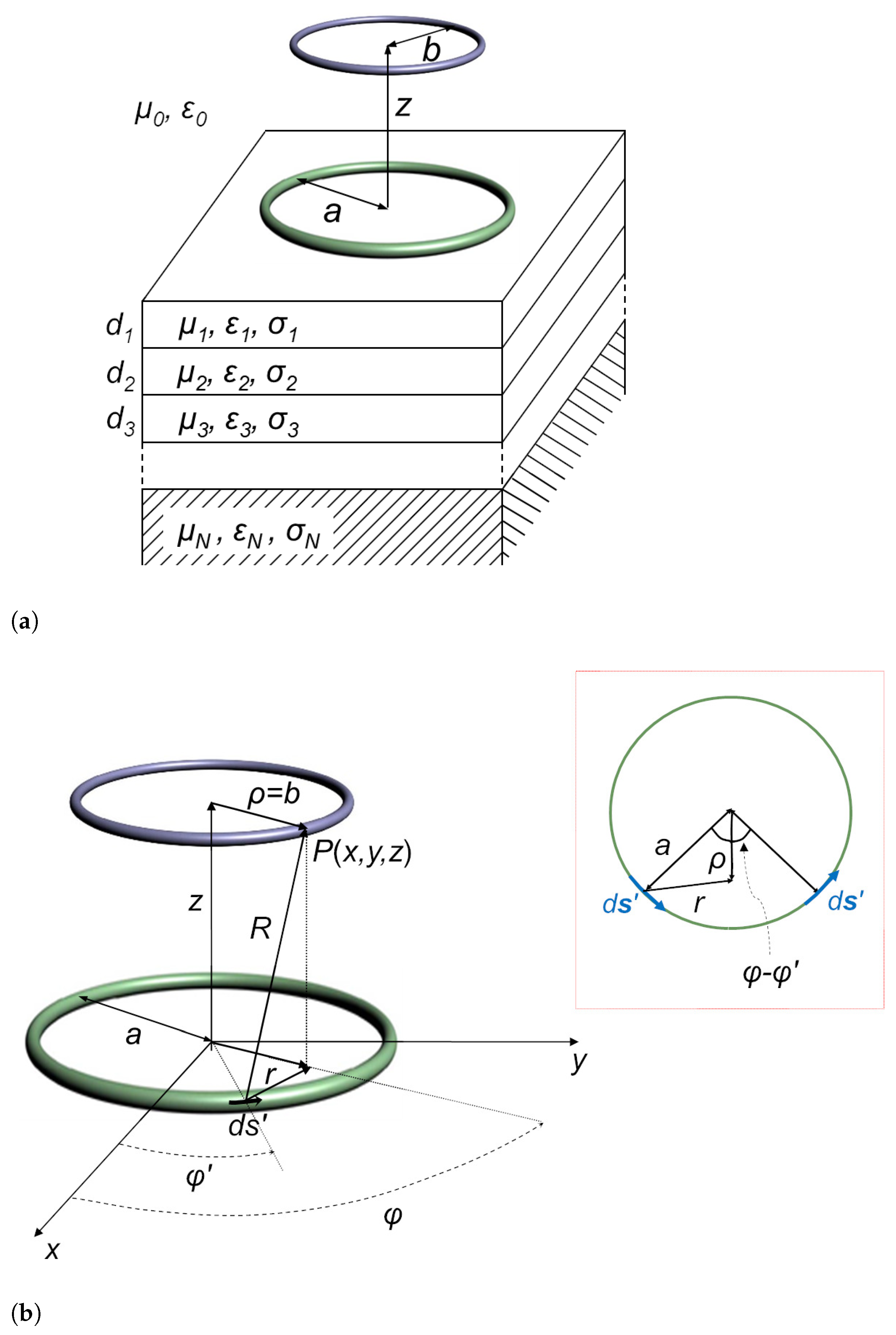
Consider two thin-wire single-turn co-axial circular coils of wire placed above a semi-infinite flat N—layer conducting medium, as shown in Figure 1. The coils, with external radii a and b (a > b), are located on the upper boundary of and at height z from the layered medium, respectively. For simplicity, only the portion of layered medium lying just below the co-axial loops is depicted in Figure 1a. The nth layer of the medium (n = $1,2,\dots ,N$) has magnetic permeability ${\mu }_n$, dielectric permittivity ${ϵ}_n$, and electrical conductivity ${\sigma }_n$, and, except for the bottom-most Nth layer, which is assumed to be unbounded downwards, has finite thickness $d_n$. Furthermore, the air space is assumed to be the zeroth layer (n = 0) of the geometrical configuration.

This section is focused on the derivation of a rigorous series-form representation for the mutual inductance of the two coils. The explicit expression must be valid and accurate regardless of the sizes of the coils and must be significantly less time-demanding than standard numerical computation algorithms, like conventional numerical integration schemes and simulation tools used to solve boundary value problems. In the theoretical development that follows, the primary loop will be assumed to be the larger loop of Figure 1. If the current in the source coil is taken to be uniform and equal to $I·e^{j\omega t}$, the magnetic flux linked with the secondary coil, with radius b, is given by

$$\begin{array}{c}\hfill M=\frac{1}{I}{\int }_S\mathit{B}\left(\mathit{r}\right)·\widehat{\mathit{n}}dS,\end{array}$$

(1)

where $\mathit{B}$ is the total magnetic flux density vector produced by the emitter in the presence of the ground, $\mathit{r}$ is the position of the generic field point P, S is the circular surface delimited by the edge of the receiving loop, and $\widehat{\mathit{n}}$ is a unit vector normal to the area element $dS$ of the surface S. The magnetic flux density vector may be expressed as

$$\begin{array}{c}\hfill \mathit{B}=\nabla \times \mathit{A},\end{array}$$

(2)

where $\mathit{A}$ is the total magnetic vector $\mathit{A}$, which may be decomposed into the sum of the primary field ${\mathit{A}}_p$ generated by the emitter plus the field ${\mathit{A}}_r$ reflected by the ground, as follows:

$$\begin{array}{c}\hfill \mathit{A}={\mathit{A}}_p+{\mathit{A}}_r.\end{array}$$

(3)

Let us introduce a rectangular $(x,y,z)$ and a cylindrical $(\rho ,\phi ,z)$ coordinate system as sketched in Figure 1b. The primary field ${\mathit{A}}_p$ at a generic point $P(x,y,z)$ is given by the superposition integral [28]

$$\begin{array}{c}\hfill {\mathit{A}}_p(\rho ,\phi ,z)=\frac{{\mu }_{0}I}{4\pi }{\int }_{C^{\prime }}\frac{e^{-j{k}_{0}R}}{R}d{\mathit{s}}^{{\displaystyle \prime }},\end{array}$$

(4)

where $C^{\prime }$ is the circumference of the source coil, $k_0=\omega \sqrt{{\mu }_0{ϵ}_0}$ is the free-space wavenumber, and R is the distance of P from the elementary current source flowing in the vector element of length $d{\mathit{s}}^{{\displaystyle \prime }}$. As shown by Figure 1b, it yields $R=\sqrt{r^2+z^2}$, with

$$\begin{array}{cc}\hfill r^2& ={(x-x^{\prime })}^2+{(y-y^{\prime })}^2\hfill \\ \hfill & \hfill ={\rho }^2+a^2-2a\rho cos\left(\phi -{\phi }^{\prime }\right),\hfill \end{array}$$

(5)

where $(x,y)$ and $(x^{\prime },y^{\prime })$ are, respectively, the rectangular coordinates of P and $d{\mathit{s}}^{{\displaystyle \prime }}$ in the $xy$—plane, related to the respective polar coordinates by the relationships

$$\begin{array}{cc}\hfill x& \hfill =\rho cos\phi ,y=\rho sin\phi ,\hfill \end{array}$$

(6)

$$\begin{array}{cc}\hfill x^{\prime }& \hfill =acos{\phi }^{\prime },y^{\prime }=asin{\phi }^{\prime }.\hfill \end{array}$$

(7)

Next, consider a pair of elements of length $d{\mathit{s}}^{{\displaystyle \prime }}$ on the emitter that are symmetrical relative to the radial distance $\rho$, as shown in the sub-figure on the right upper corner of Figure 1b. Since the two elementary vectors are equally spaced from the field point, and the components of the vectors along the $\rho$—direction cancel out, it is deduced that the total contribution from the pair of point sources to ${\mathit{A}}_p$ is directed perpendicular to $\rho$ (that is in the $\phi$—direction only). This means that ${\mathit{A}}_p$ may be obtained by summing up only the components of the elementary contributions $d{\mathit{A}}_p$ that are directed in the $\phi$—direction. It yields

$$\begin{array}{cc}{\mathit{A}}_p=A_{\phi }^{\left(p\right)}\widehat{\mathit{\phi }}\hfill & =\frac{{\mu }_{0}I}{4\pi }{\int }_{C^{\prime }}\frac{e^{-j{k}_{0}R}}{R}cos\left(\phi -{\phi }^{\prime }\right)d{s}^{\prime }\widehat{\mathit{\phi }}\hfill \\ \hfill & =\frac{{\mu }_{0}Ia}{2\pi }{\int }_0^{\pi }\frac{e^{-j{k}_{0}R}}{R}cos\left(\phi -{\phi }^{\prime }\right)d{\phi }^{\prime }\widehat{\mathit{\phi }}\hfill \end{array}$$

(8)

with $\widehat{\mathit{\phi }}$ and $cos(\phi -{\phi }^{\prime })d{s}^{{\displaystyle \prime }}$ being, respectively, the unit vector in the $\phi$—direction and the $\phi$—component of $d{\mathit{s}}^{\prime }$, and where account has been taken that $d{s}^{\prime }=ad{\phi }^{\prime }$.

It should be noted that since the current I in the emitter has been assumed to be uniform, the radiated field does not depend on the observation angle $\phi$. This implies that the electromagnetic (EM) field described by (8) is transverse electric (TE) with respect to the $z$—direction, as the electric field has no vertical component. In fact, the primary electric field vector may be expressed as N. 1.122 in [28]

$$\begin{array}{c}\hfill {\mathit{E}}_p=-j\omega {\mu }_0{\mathit{A}}_p+\frac{1}{j\omega {ϵ}_0}\nabla \left(\nabla ·{\mathit{A}}_p\right),\end{array}$$

(9)

and, since ${\mathit{A}}_p$ consists only of a $\phi$-component which does not depend on $\phi$, its divergence is identically null. Consequently, ${\mathit{E}}_p$ has the same direction as ${\mathit{A}}_p$ and is perpendicular to z. It is now convenient to perform the following replacement 2.9 in [28]

$$\begin{array}{c}\hfill \frac{e^{-j{k}_{0}R}}{R}=\frac{1}{2\pi }{\int }_{-\infty }^{\infty }{\int }_{-\infty }^{\infty }\frac{1}{u_0}{e}^{-u_0\left|z\right|}{e}^{-j\left[k_x(x-x^{\prime })+k_y(y-y^{\prime })\right]}d{k}_{x}d{k}_y\end{array}$$

(10)

in (8), with $u_0=\sqrt{k_x^2+k_y^2-k_0^2}$. This makes it possible, after interchanging the order of the integrals, to rewrite the primary field as a sum of plane waves with continuously varying angles of incidence, namely

$$\begin{array}{c}\hfill A_{\phi }^{\left(p\right)}=\frac{{\mu }_{0}Ia}{4{\pi }^2}{\int }_{-\infty }^{\infty }{\int }_{-\infty }^{\infty }\frac{1}{u_0}{e}^{-u_0\left|z\right|}\left\{{\int }_0^{\pi }{e}^{-j\left[k_x(x-x^{\prime })+k_y(y-y^{\prime })\right]}cos\left(\phi -{\phi }^{\prime }\right)d{\phi }^{\prime }\right\}d{k}_{x}d{k}_y,\end{array}$$

(11)

and to find an analogous expression for the field reflected by the ground. In fact, each TE plane wave of the spectrum gives rise to a reflected wave, with a reflection coefficient at the top surface of the material medium given by N. 4.19 in [28]

$$\begin{array}{c}\hfill R_{TE}=\frac{Y_0-{\widehat{Y}}_1}{Y_0+{\widehat{Y}}_1},\end{array}$$

(12)

where

$$\begin{array}{c}\hfill Y_n=\frac{u_n}{j\omega {\mu }_n}\end{array}$$

(13)

is the intrinsic admittance of the nth layer, and with

$$\begin{array}{}\mathrm{(14)}& u_n=\sqrt{k_x^2+k_y^2-k_n^2},Re\left[u_n\right]>0,\hfill \mathrm{(15)}& k_n^2=-j\omega {\mu }_n\left({\sigma }_n+j\omega {ϵ}_n\right),\hfill \end{array}$$

being ${\sigma }_0=0$. On the other hand, ${\widehat{Y}}_n$ is the surface admittance at the upper surface of the nth layer and is defined by the recurrence relationship

$$\begin{array}{c}\hfill {\widehat{Y}}_n=Y_n\frac{{\widehat{Y}}_{n+1}+Y_n\tanh \left(u_n{d}_n\right)}{Y_n+{\widehat{Y}}_{n+1}\tanh \left(u_n{d}_n\right)},n=N-1,\dots ,1,\end{array}$$

(16)

where $d_1,d_2,\dots ,d_{N-1}$ are the thicknesses of the $N-1$ finite layers, and ${\widehat{Y}}_N=Y_N$.

With the use of (12), the reflected potential may be expressed as

$$\begin{array}{c}\hfill A_{\phi }^{\left(r\right)}=\frac{{\mu }_{0}Ia}{4{\pi }^2}{\int }_{-\infty }^{\infty }{\int }_{-\infty }^{\infty }\frac{R_{TE}}{u_0}{e}^{-u_{0}z}\left\{{\int }_0^{\pi }{e}^{-j\left[k_x(x-x^{\prime })+k_y(y-y^{\prime })\right]}cos\left(\phi -{\phi }^{\prime }\right)d{\phi }^{\prime }\right\}d{k}_{x}d{k}_y,\end{array}$$

(17)

and, since $z>0$ in the air space, it is straightforward to sum the two contributions $A_{\phi }^{\left(p\right)}$ and $A_{\phi }^{\left(r\right)}$, to obtain the total field

$$\begin{array}{cc}{A}_{\phi }\hfill & =\frac{{\mu }_{0}Ia}{4{\pi }^2}{\int }_{-\infty }^{\infty }{\int }_{-\infty }^{\infty }\frac{1+R_{TE}}{u_0}{e}^{-u_{0}z}\left\{{\int }_0^{\pi }{e}^{-j\left[k_x(x-x^{\prime })+k_y(y-y^{\prime })\right]}cos\left(\phi -{\phi }^{\prime }\right)d{\phi }^{\prime }\right\}d{k}_{x}d{k}_y\hfill \\ \hfill & =\frac{{\mu }_{0}Ia}{2{\pi }^2}{\int }_0^{\pi }\left\{{\int }_{-\infty }^{\infty }{\int }_{-\infty }^{\infty }\frac{e^{-u_{0}z}}{u_0+j\omega {\mu }_0{\widehat{Y}}_1}{e}^{-j\left[k_x(x-x^{\prime })+k_y(y-y^{\prime })\right]}d{k}_{x}d{k}_y\right\}cos\left(\phi -{\phi }^{\prime }\right)d{\phi }^{\prime }.\hfill \end{array}$$

(18)

Since the quantity within the curly brackets in (18) is an inverse 2-D Fourier transform of the function

$$\begin{array}{c}\hfill F\left(k_x^2+k_y^2\right)=\frac{e^{-u_{0}z}}{u_0+j\omega {\mu }_0{\widehat{Y}}_1},\end{array}$$

(19)

the following relationship, valid for circularly symmetric functions to be transformed, may be applied [31]

$$\begin{array}{c}\hfill {\int }_{-\infty }^{\infty }{\int }_{-\infty }^{\infty }F\left(k_x^2+k_y^2\right)e^{-j\left[k_x(x-x^{\prime })+k_y(y-y^{\prime })\right]}d{k}_{x}d{k}_y=2\pi {\int }_0^{\infty }F\left(\lambda \right)J_0\left(\lambda r\right)\lambda d\lambda ,\end{array}$$

(20)

and, consequently, it is found that

$$\begin{array}{cc}\hfill A_{\phi }& \hfill =\frac{{\mu }_{0}Ia}{\pi }{\int }_0^{\pi }\left\{{\int }_0^{\infty }\frac{e^{-u_{0}z}}{u_0+j\omega {\mu }_0{\widehat{Y}}_1}{J}_0\left(\lambda r\right)\lambda d\lambda \right\}cos\left(\phi -{\phi }^{\prime }\right)d{\phi }^{\prime },\hfill \end{array}$$

(21)

where $J_0\left(\zeta \right)$ is the zeroth-order Bessel function and $\lambda =\sqrt{k_x^2+k_y^2}$. Expression (21) for the vector potential may now be used in combination with (1) and (2) to evaluate the mutual inductance. First, substituting (2) into (1) and applying Stokes’s theorem provides

$$\begin{array}{cc}M\hfill & =\frac{1}{I}{\int }_S\left[\mathbf{\nabla }\times \mathit{A}\left(\mathit{r}\right)\right]·\widehat{\mathit{n}}dS\hfill \\ \hfill & =\frac{1}{I}{\int }_C\mathit{A}\left(\mathit{r}\right)·d\mathit{s}\hfill \end{array}$$

(22)

where C is the circumference of the receiving loop and $d\mathit{s}$ is a vector element of length along C. Then, use of (21) into (22) allows the expression of M in the form

$$\begin{array}{c}\hfill M=\frac{{\mu }_{0}a}{\pi }{\int }_C\underset{A_{\phi }}{\underbrace{{\int }_0^{\pi }\left\{{\int }_0^{\infty }\frac{e^{-u_{0}z}}{u_0+j\omega {\mu }_0{\widehat{Y}}_1}{J}_0\left(\lambda r\right)\lambda d\lambda \right\}cos(\phi -{\phi }^{\prime })d{\phi }^{\prime }}}\widehat{\mathit{\phi }}·d\mathit{s},\end{array}$$

(23)

which, after taking into account that $d\mathit{s}=bd\phi \widehat{\mathit{\phi }}$ and that, for points belonging to C, $\rho =b$ (as shown by Figure 1b), is turned into

$$\begin{array}{c}\hfill M=\frac{{\mu }_{0}a}{\pi }{\int }_0^{2\pi }bd\phi \underset{A_{\phi }}{\underbrace{{\int }_0^{\pi }cos(\phi -{\phi }^{\prime })d{\phi }^{\prime }{\int }_0^{\infty }\frac{e^{-u_{0}z}}{u_0+j\omega {\mu }_0{\widehat{Y}}_1}{J}_0\left(\lambda {\left.r\right|}_{\rho =b}\right)\lambda d\lambda }}.\end{array}$$

(24)

It should be noted that, as previously observed, $A_{\phi }$ is not a function of $\phi$, which implies that any value of $\phi$ can be chosen to calculate it. Hence, for simplicity we will assume $\phi =0$ in the integrand of (24), which leads to write

$$\begin{array}{c}\hfill M=2{\mu }_{0}ab{\int }_0^{\pi }cos{\phi }^{\prime }d{\phi }^{\prime }{\int }_0^{\infty }\frac{e^{-u_{0}z}}{u_0+j\omega {\mu }_0{\widehat{Y}}_1}{J}_0\left(\lambda c\right)\lambda d\lambda ,\end{array}$$

(25)

with

$$\begin{array}{c}\hfill c=\sqrt{a^2+b^2-2abcos{\phi }^{\prime }}.\end{array}$$

(26)

To evaluate the double integral in (25), it suffices to use the Lth-order rational approximation

$$\begin{array}{c}\hfill \frac{e^{-u_{0}z}}{u_0+j\omega {\mu }_0{\widehat{Y}}_1}\cong \sum _{l=1}^L\frac{r_l}{j{\lambda }^2-p_l},Re\left[p_l\right]<0,\end{array}$$

(27)

obtained using the least squares-based fitting method presented in [30]. The replacement (27) allows the rewriting of M in the form

$$\begin{array}{c}\hfill M=2{\mu }_{0}ab\sum _{l=1}^L{r}_l{\int }_0^{\pi }cos{\phi }^{\prime }d{\phi }^{\prime }{\int }_0^{\infty }\frac{1}{j{\lambda }^2-p_l}{J}_0\left(\lambda c\right)\lambda d\lambda ,\end{array}$$

(28)

whose inner integral is tabulated and given by p. 671, N. 6.536.4 in [32]

$$\begin{array}{c}\hfill {\int }_0^{\infty }\frac{1}{j{\lambda }^2-p_l}{J}_0\left(\lambda c\right)\lambda d\lambda =-\frac{\pi }{2}{H}_0^{\left(2\right)}\left(-jc\sqrt{j{p}_l}\right),\end{array}$$

(29)

with $H_{\nu }^{\left(2\right)}\left(\zeta \right)$ being the $\nu$th-order Hankel function of the second kind. Finally, use of (29) in conjunction with Gegenbauer addition theorem p. 361, N. 11.3.6 in [33]

$$\begin{array}{c}\hfill H_0^{\left(2\right)}\left(-jc\sqrt{j{p}_l}\right)=\sum _{m=-\infty }^{\infty }{H}_m^{\left(2\right)}(-ja\sqrt{j{p}_l})J_m(-jb\sqrt{j{p}_l})cosm{\phi }^{\prime }\end{array}$$

(30)

into (28), provides

$$\begin{array}{cc}M(a,b,z)\hfill & =-\pi {\mu }_{0}ab\sum _{l=1}^L{r}_l\sum _{m=-\infty }^{\infty }{H}_m^{\left(2\right)}(-ja\sqrt{j{p}_l})J_m(-jb\sqrt{j{p}_l}){\int }_0^{\pi }cosm{\phi }^{\prime }cos{\phi }^{\prime }d{\phi }^{\prime }\hfill \\ \hfill & =-\frac{\pi {\mu }_{0}ab}{2}\sum _{l=1}^L{r}_l\sum _{m=-\infty }^{\infty }{H}_m^{\left(2\right)}(-ja\sqrt{j{p}_l})J_m(-jb\sqrt{j{p}_l}){\int }_{-\pi }^{\pi }cosm{\phi }^{\prime }cos{\phi }^{\prime }d{\phi }^{\prime }\hfill \\ \hfill & -{\pi }^2{\mu }_{0}ab\sum _{l=1}^L{r}_l{H}_1^{\left(2\right)}(-ja\sqrt{j{p}_l})J_1(-jb\sqrt{j{p}_l}),\hfill \end{array}$$

(31)

where account has been taken that the mth ${\phi }^{\prime }$—integral is non-null, and equal to $\pi$, only for $m=\pm 1$, and that $H_{-1}^{\left(2\right)}\left(\zeta \right)=-H_1^{\left(2\right)}\left(\zeta \right)$ and $J_{-1}\left(\zeta \right)=-J_1\left(\zeta \right)$ [34].

It should be observed that the poles $p_l$ and the residues $r_l$ of the rational approximation (27) depend on the coil-to-coil spacing z as well as on the electromagnetic properties of the layered medium. However, this dependence is not made explicit in (31) for notational simplicity.

It should also be noted that the derived expression (31) may be generalized to the case where the source and/or the receiver is a multi-turn flat pancake coil. For instance, consider the geometrical configuration shown in Figure 2. Here, the receiver, which lies together with the emitter on the top surface of a non-magnetic homogeneous ground, is made up of $N_b$ turns with radii $b_l(l=1,2,\dots ,N_b)$. In such a situation, the mutual inductance of the two coils may be expressed as [35]

$$\begin{array}{c}\hfill M_{tot}=\sum _{l=1}^{N_b}M(a,b_l,0),\end{array}$$

(32)

where $M(a,b_l,0)$ is given by (31).

Finally, it should be observed that, in the absence of the ground, (25) may be exactly evaluated starting from applying the identity 11.41.17 in [33]

$$\begin{array}{c}\hfill {\int }_0^{\pi }{J}_0\left(\lambda c\right)cos{\phi }^{\prime }d{\phi }^{\prime }=\pi J_1\left(\lambda a\right)J_1\left(\lambda b\right),\end{array}$$

(33)

which permits the achievement of the compact representation

$$\begin{array}{c}\hfill M=2\pi {\mu }_{0}ab{\int }_0^{\infty }\frac{e^{-u_{0}z}}{u_0+j\omega {\mu }_0{\widehat{Y}}_1}{J}_1\left(\lambda a\right)J_1\left(\lambda b\right)\lambda d\lambda .\end{array}$$

(34)

Then, after setting $k_n=k_0(n=1,2,\dots ,N)$ and ${\widehat{Y}}_1=Y_0$, (34) assumes the form

$$\begin{array}{c}\hfill M_{free-space}(a,b)=\pi {\mu }_{0}ab{\int }_0^{\infty }\frac{e^{-u_{0}z}}{u_0}{J}_1\left(\lambda a\right)J_1\left(\lambda b\right)\lambda d\lambda ,\end{array}$$

(35)

whose explicit form, in the quasi-static limit, reads [35]

$$\begin{array}{c}\hfill M_{free-space}(a,b)={\mu }_0\sqrt{ab}\left[\left(\frac{2}{\kappa }-\kappa \right)K\left(\kappa \right)-\frac{2}{\kappa }E\left(\kappa \right)\right],\end{array}$$

(36)

with

$$\begin{array}{c}\hfill \kappa =\sqrt{\frac{4ab}{{(a+b)}^2+z^2}},\end{array}$$

(37)

and where $K\left(\kappa \right)$ and $E\left(\kappa \right)$ are the complete elliptic integrals of the first and second kind, respectively.

3. Results and Discussion

The validation of the developed theory is carried out by comparing its outcomes with the data generated by the finite-difference time-domain (FDTD) method, and those originating from numerical integration of (34) through an adaptive G7-K15 Gauss–Kronrod quadrature scheme. The calculations are performed on a machine with a 1.8 GHz processor and a RAM capability of 32 GB. At first, two co-axial coils with radii $a=2$ m and $b=1$ m are considered, and the real and imaginary parts of M are calculated and plotted against the operating frequency. The receiver is positioned at height $z=10$ cm above the ground, which is assumed to be a two-layer medium ($N=2$) with ${\sigma }_1=100$ mS/m, ${\sigma }_2=10$ mS/m, ${ϵ}_1={ϵ}_2=10{ϵ}_0$, and ${\mu }_1={\mu }_2={\mu }_0$. Moreover, the thickness $d_1$ of the first layer of the medium is taken to be equal to 5 m. The three-dimensional FDTD mesh is configured with 200 × 200 × 20 cubic cells, 5 cm in size, spanning a spatial domain of 10 × 10 × 1 m centered at the center of the coils. Perfectly matched layer (PML) absorbing boundary conditions are assumed at the computational boundaries, and the time step is taken to be $\Delta t=90$ ps, which is below the Courant limit, namely p.135 in [36]

$$\begin{array}{c}\hfill \Delta t_{\genfrac{}{}{0pt}{}{stable}{limit}}=\frac{1}{c\sqrt{\frac{1}{{\Delta x}^2}+\frac{1}{{\Delta y}^2}+\frac{1}{{\Delta z}^2}}}=\frac{\Delta x}{c\sqrt{3}}\cong 96\mathrm{ps}\end{array}$$

(38)

with $c=3·{10}^8$ m/s being the speed of light in vacuum, and where account has been taken that, for cubic cells, $\Delta x=\Delta y=\Delta z=5$ cm. The primary coil is modeled as a distribution of impressed current sources, and a sine-modulated Gaussian waveform is used to describe its dependence on time. The $H_z$—field is sampled in the time interval $T_s=2^{16}\Delta t$, and numerical integration is then performed along the area delimited by the receiver. Finally, the Fast Fourier Transform (FFT) is applied to provide the spectrum of the sampled mutual inductance between the coils.

On the other hand, the length of the sum of partial fractions in (27) is taken to be $L=12$. Its poles $p_l$ and residues $r_l$, to be used in (31), are calculated through an iterative method consisting of the repeated application of the fitting procedure in [30], until the root mean square (RMS) relative error of the approximation (27) does not exceed the threshold of ${10}^{-3}$. The guess values of the poles at the beginning of the iterative process are $p_l=(-1+j{q}_l)$$m^{-2}$$(l=1,2,\dots ,12)$, with the $q_l$’s linearly distributed in the interval comprised between −10 m⁻² and 10 m⁻². With the chosen values of the starting poles, the process is terminated after 13 iterations when the error exhibited by (27) is equal to about 10⁻⁶, which means that the 12th-order approximation in (27) gives rise to an accurate fitting of the integrand of the field integral.

The frequency spectra of the real and imaginary parts of M, computed using (31), the FDTD method, and numerical integration of (34), are illustrated in Figure 3. Here, the trends corresponding to lower-order rational approximations (27) (second- and fourth-order approximations, namely) are also depicted. As is seen, the trends from the derived expression for M approach the outcomes from both the FDTD method and numerical integration as L is increased, and excellent agreement is obtained for $L=12$. This means that few terms are required in (31) to obtain extremely accurate results, provided that the primary loop can support a uniform current. This requirement is always fulfilled every time that the length of the wire constituting the loop is much smaller than the wavelength in free space, say smaller than one third of the wavelength [9]. In other words, the inequality $k_{0}a<1/3$ must be fulfilled. This condition tells us that (34) and (31) may be always used every time that

$$\begin{array}{c}\hfill \frac{\omega a}{c}<\frac{1}{3}\end{array}$$

(39)

that is, in the case of the considered example, when

$$\begin{array}{c}\hfill f<\frac{c}{6\pi a}=\frac{3·{10}^8}{12\pi }\cong 8\mathrm{MHz}.\end{array}$$

(40)

Beyond the frequency of 8 MHz, the variations of the current along the emitter become non-negligible and, in principle, (34) and (31) could not be used anymore. However, this restriction on the frequency range of validity of (31) may be relaxed if a uniform current is imposed by the feeding system [37,38]. Hence, the proposed approach can be used at least up to the frequency limit imposed by (39), and to the extent that the source coil can support a uniform current, the validity of (31) is not affected by the operating frequency.

Figure 3a also points out that, in the low-frequency region, the trend of the real part of M, as it comes from (31) with $L=12$ and from numerical simulations, becomes horizontal and in agreement with the curve produced by the solution (36), valid for coils embedded in free-space. This is because, at low frequencies, the effects due to the skin depth in the medium, as well as those associated with the displacement currents, are negligible, which means that $|k_n|a<<1$ and $|k_n|b<<1$ ($n=1,2$). Since all these conditions are met when $|k_1|a<<1$, an estimate of the frequency interval where the free-space solution (36) holds, i.e., the range where the presence of the ground can be neglected, may be found by solving the inequality

$$\begin{array}{c}\hfill |k_1|a\cong a\sqrt{\omega {\mu }_0{\sigma }_1}=\frac{a\sqrt{2}}{{\delta }_1}<\frac{1}{3}\end{array}$$

(41)

for the operating frequency, which leads to

$$\begin{array}{c}\hfill f<\frac{1}{18\pi a^2{\mu }_0{\sigma }_1}=\frac{{10}^8}{288{\pi }^2}\cong 35.2\mathrm{kHz}.\end{array}$$

(42)

As confirmed by Figure 3a, the trends from (31) and (36) start to diverge at a frequency approximately equal to 35 kHz.

Although (31) has been proven to offer the same degree of accuracy as the considered numerical procedures, it is revealed to be advantageous over the latter in terms of time cost. This point is illustrated by

Table 1. CPU time comparisons for the calculation of M against frequency.

Approach	CPU Time [s]	Speed-Up Compared to FDTD	Speed-Up Compared to G7-K15
FDTD (200 × 200 × 20)	38.6	-	0.57
G7-K15	22.1	1.75	-
(31) with $L=2$	2.87 × 10${}^{-2}$	1345	770
(31) with $L=4$	6.93 × 10${}^{-2}$	557	319
(31) with $L=12$	1.74	22.2	12.7
(31) with $L=16$	3.12	12.4	7.08

, which shows the computation times required by the proposed approach, Gaussian integration, and the FDTD method to calculate the profiles depicted in Figure 3. The speed-up offered by the new hybrid approach with respect to the two purely numerical methods is also shown. As is seen, the time cost of (31) is significantly smaller than those of both the numerical procedures and that, in particular, the speed-up offered by (31) with respect to the FDTD method is equal to about 22 when $L=12$, i.e., when the trends from the two approaches are overlapping. On the other hand, the derived formula with $L=12$ is more than 12 times faster than the Gauss–Kronrod rule. These data confirm that (31) consistently outperforms the FDTD method and Gaussian integration regarding the computational burden.

One would ask whether the developed formulation still provides accurate results if the geometrical parameters of the two-coil system are changed. This aspect is illustrated in Figure 4, which depicts the impact of changing the radius b of the receiver on the mutual inductance M. In this example, both the coils lie on the material medium, which is assumed to be a single-layer medium with ${\sigma }_1=100$ mS/m, ${ϵ}_1=10{ϵ}_0$, and ${\mu }_1={\mu }_0$. The emitter has radius $a=2$ m and operates at the frequency $f=10$ MHz. The radius of the receiver varies between 1 cm and 120 cm. Figure 4a,b show profiles of the real and imaginary parts of M against b, calculated using (31), the G7-K15 quadrature scheme, the free-space solution (36), and the preceding quasi-static solution to the problem, obtained by assuming that the receiver is physically as well as electrically small. This hypothesis permits the calculation of the inductance as the $H_z$—field at the center of the emitter multiplied by the area enclosed by the receiver, i.e., as $M={\mu }_0\pi b^2{H}_z^0$, where $H_z^0$ is given by [28]

$$\begin{array}{c}\hfill H_z^0=-\frac{1}{k_1^2{a}^3}\left[3-\left(3+3j{k}_{1}a-k_1^2{a}^2\right)e^{-j{k}_{1}a}\right].\end{array}$$

(43)

The curves plotted in Figure 4 confirm the adherence of the results produced by the proposed analytical approach to the numerical data. Conversely, it is also noticed how the profiles of the real and imaginary parts of M arising from the small-loop approximation are inadequate in a significant portion of the considered range of b, i.e., where the assumption of the small receiver fails. In fact, the receiver is both physically and electrically small as long as its radius is much smaller than that of the emitter ($b<<a$) and, at the same time, $k_{0}b<<1$, i.e., $k_{0}b<1/3$ [9]. At the chosen frequency of 10 MHz, the latter condition translates into the inequality

$$\begin{array}{c}\hfill b<\frac{\lambda }{6\pi }=\frac{c}{6\pi f}=\frac{3·{10}^8}{6\pi ·{10}^7}\cong 160\mathrm{cm},\end{array}$$

(44)

which is always true as b is included in the 1 cm ≤ b ≤ 120 cm range. Instead, the former condition implies that the receiver radius b must be at least ten times smaller than the radius a of the emitter, which is at most equal to about 20 cm. For larger values of b, the small-loop approximation is expected to produce inaccurate results, and this is confirmed by the data plotted in Figure 4a,b. As is seen, the small-loop approximation leads to underestimating both the real part and the imaginary part (in absolute value) of the inductance.

The data plotted in Figure 4a also reveals that, at intermediate or high frequencies, neglecting the presence of the ground using the free-space solution (36) always leads to overestimating the magnetic coupling. In fact, a significant discrepancy is observed between the outcomes of (36) and those provided by (31) and G7-K15 numerical scheme, and the presence of the ground has the effect of breaking down the flux linkage between the loops.

Furthermore, Figure 4 also permits the study of the behavior of the magnetic coupling between the coils as b is changed. The plotted $b$—profiles clearly highlight that, at the frequency of 10 MHz, both the real and the imaginary parts of the mutual inductance increase in absolute value with increasing b, even if they are opposite in sign. In fact, while the imaginary part is negative and decreasing, the real part is positive and always grows up.

The degree of accuracy of the proposed solution is further investigated by Figure 5, which illustrates the relative error arising from using (31) and (43) in place of numerical integration of (34), plotted against the receiver radius b. As shown by Figure 5a, the relative percent error of the real part of (43) is about $30\%$ for $b=20$ cm, and it dramatically grows up for larger receivers, up to become slightly less than $70\%$ when $b=40$ cm and, finally, up to exceed $90\%$ if $b>80$ cm. Analogous conclusions may be drawn from the data plotted in Figure 5b. Here, the relative percent error associated with the imaginary part of (43) is less than $2\%$ for $b=20$ cm, but it reaches $20\%$ for $b=80$ cm and $40\%$ for $b=140$ cm. On the other hand, for a given value of L, even the relative error generated by (31) monotonically grows as b is increased. However, the error is significantly smaller than that produced by (43) and can always be reduced by increasing the order L of the approximation in (27). Thus, the curves of Figure 5 confirm that the outcomes from (31) converge to the exact data and tell us that convergence is faster for lower values of the receiver radius b. This does not mean that slow convergence is observed for larger receivers. As an example, for $b=1$ m, it suffices to choose $L=12$ to make the relative errors exhibited by the real and imaginary parts of (31) equal to 4.5‰ and 0.3‰, respectively. The reasonable relative error generated by (31) for $L=12$, $a=2$ m, and $b=1$ m, is counterbalanced by the speed-up offered with respect to Gauss–Kronrod rule, which, as previously noticed, is equal to 12.7. Furthermore, as pointed out by Figure 5, increasing L up to 16 allows the reduction of the relative errors of the real and imaginary parts down to $5\times {10}^{-4}$ and $2.7\times {10}^{-5}$. This is not obtained at the price of significantly decreasing the speed-up with respect to purely numerical techniques. In fact, as pointed out by Table 1, the time cost of (31) is still about seven times smaller than that implied by the Gauss–Kronrod numerical scheme.

Finally, the developed theory may be used to acquire helpful information about the impact of soil conductivity on the mutual coupling between the coils. This aspect is investigated by Figure 6, which shows the real and imaginary components of the mutual inductance of two loops positioned on a homogeneous medium, plotted versus the electrical conductivity ${\sigma }_1$. Here, the concentric coils have radii $a=2$ m (source) and $b=1$ m (receiver), and the source coil still operates at 10 MHz. It is assumed ${ϵ}_1=10{ϵ}_0$, while ${\sigma }_1$ can span a wide range, from 1 mS/m to 1 S/m. The calculations are performed using numerical integration of (34), the small-loop approximation (43), and the new solution (31), with the order L of the rational approximation still taken as a parameter. The profiles depicted in Figure 6 show that, at the frequency of 10 MHz, the impact of changing ${\sigma }_1$ on the magnetic coupling is not negligible. In particular, the real part of the inductance, positive in sign, decreases as ${\sigma }_1$ is increased up to about $\sigma \le 100$ mS/m. Thereinafter, it does not substantially change any longer, and its trend becomes nearly horizontal. On the other hand, the imaginary part is negative in sign and exhibits different behaviors depending on the values of ${\sigma }_1$. It decreases (increases in absolute value) with increasing ${\sigma }_1$ if the latter is sufficiently small. Next, it starts to decrease less and less as ${\sigma }_1$ is increased until a minimum is reached. Then, it monotonically grows up and its absolute value decreases.

It is also noted that, in this example, Formula (43) gives inaccurate results all over the considered range for ${\sigma }_1$. This should be expected, as the receiver radius, equal to 2 m, is only twice that of the receiver (1 m), which means that the small-loop assumption does not hold.

4. Conclusions

This work has presented an accurate series-form representation for the mutual inductance of two co-axial coils in the presence of an arbitrarily layered conductive ground. The expression has been obtained through a rigorous quasi-analytical procedure. Starting from the Biot–Savart expression for the primary vector potential generated by the source coil, the integral representation for the potential reflected by the layered ground has been derived, and the resulting total vector potential has then been integrated along the external circumference of the receiving coil. The resulting double-integral representation for the inductance has then been evaluated analytically by applying the Gegenbauer addition theorem once the term of the integrand that contains branch cuts has been replaced with an accurate, rational approximation provided by a well-established least squares-based fitting technique.

The outcomes from the derived explicit solution have been shown to be in excellent agreement with the numerical data produced by the FDTD method and the Gauss–Kronrod quadrature rule. It has also been pointed out how the derived expression permits the reduction of the computation time with respect to the FDTD method and the Gauss–Kronrod rule, respectively, by 22 and 12 times while maintaining the same degree of accuracy as the two numerical approaches. Finally, limited to the single-layer medium case, the conducted numerical tests have shown that the new solution is still accurate, whereas the well-known small-loop approximation for the inductance fails, i.e., when the receiver radius b is no longer small and becomes comparable to the radius of the emitter. The analysis has also revealed that, in general, the small-loop approximation leads to underestimating mutual inductance.