Abstract
As the urgency to adopt renewable energy sources escalates, so does the need for accurate forecasting of power output, particularly for wind and solar power. Existing models often struggle with noise and temporal intricacies, necessitating more robust solutions. In response, our study presents the SL-Transformer, a novel method rooted in the deep learning paradigm tailored for green energy power forecasting. To ensure a reliable basis for further analysis and modeling, free from noise and outliers, we employed the SG filter and LOF algorithm for data cleansing. Moreover, we incorporated a self-attention mechanism, enhancing the model’s ability to discern and dynamically fine-tune input data weights. When benchmarked against other premier deep learning models, the SL-Transformer distinctly outperforms them. Notably, it achieves a near-perfect value of 0.9989 and a significantly low SMAPE of 5.8507% in wind power predictions. For solar energy forecasting, the SL-Transformer has achieved a SMAPE of 4.2156%, signifying a commendable improvement of 15% over competing models. The experimental results demonstrate the efficacy of the SL-Transformer in wind and solar energy forecasting.
1. Introduction
Renewable energy sources such as wind power and solar power are increasingly being integrated into microgrids to reduce reliance on traditional fossil fuels and mitigate environmental impacts [1,2]. However, the variability and intermittency of wind power generation can cause challenges for microgrid operation and stability, especially in power forecasting. Time-series power forecasting is a critical task in microgrid operation, enabling efficient and reliable scheduling of renewable energy sources and grid resources. The accuracy of power forecasting has significant implications for the efficient and reliable operation of microgrids, making it a highly researched and active area of study [3].
Despite the importance of power forecasting for microgrid wind turbine units, accurate and reliable forecasting remains a significant challenge due to several factors [4,5]. First, the output of wind or solar power is highly variable and intermittent, making it difficult to predict power demand accurately [6]. Secondly, the power prediction of wind power and photovoltaic power generation in the power grid needs to consider various factors, such as weather conditions and power supply fluctuations, which further increases the complexity of the forecasting task [7]. Third, the lack of historical data and the limited availability of real-time data pose significant challenges to developing accurate power forecasting models [8]. Fourth, traditional statistical models often fail to capture the complex and nonlinear relationships between the different variables, further reducing the accuracy of power forecasting [9]. These challenges highlight the need to develop more advanced and accurate power forecasting models that can address the limitations of traditional approaches and improve the efficiency and reliability of wind and solar power generation in the microgrid [10,11,12].
In response to the aforementioned challenges, traditional filtering methods play a pivotal role in the preprocessing stage by mitigating noise and outlier values in the sensor acquisition process, thereby establishing a robust foundation for subsequent predictive modeling. These conventional filtering techniques, through processes of data smoothing and outlier detection, effectively cleanse the power data, furnishing the predictive model with more accurate and stable inputs. Notably, the Savitzky–Golay filter finds wide application in the smoothing of wind speed data, utilizing local polynomial fitting to eliminate noise and spurious fluctuations [13,14]. Conversely, the Local Outlier filter is employed for solar power generation data to detect and eliminate outliers, thereby reducing interference and noise in the data [15]. By comprehensively employing these signal processing methods, more reliable and accurate wind power and solar power data are provided, laying the foundation for subsequent green energy predictions.
Traditionally, power forecasting of green energy has been accomplished using statistical time-series models such as ARIMA, SARIMA, and exponential smoothing methods. These methods rely on historical power data to capture the seasonal and temporal trends in power demand, making them suitable for short-term forecasting [16,17]. However, they fail to capture the complex and nonlinear relationships between the various factors affecting power demand, such as weather patterns and power supply fluctuations. Additionally, these methods are based on assumptions of stationarity and linearity, which may not be true for wind and solar power generation in the grid [18]. Despite these limitations, these traditional methods remain popular due to their simplicity and ease of use. Therefore, due to the above factors, they may not be suitable for power forecasting of wind and solar power generation, and more advanced and accurate methods need to be developed [19,20].
With the development of machine learning technologies, methods such as artificial neural networks, support vector machines, decision trees, and random forests have emerged as powerful tools for wind and solar energy power forecasting [21,22,23,24]. These methods can handle multidimensional, nonlinear, and non-stationary power data more effectively, thereby improving the accuracy and reliability of predictions. For instance, artificial neural networks, by constructing complex multi-layered neural network structures, can learn abstract features from the data and exhibit outstanding performance in power forecasting [25,26]. However, traditional machine learning techniques still possess certain limitations, such as the need for substantial amounts of data and computational resources, as well as complex model structures with limited interpretability [27]. This has prompted both academia and industry to shift towards more powerful deep learning methods.
Deep learning techniques have shown remarkable potential in wind and solar power forecasting [28]. By constructing deep neural network structures, deep learning models can extract highly abstract features from massive datasets, capturing the complex relationships between power and renewable energy sources. Recently, deep learning models like LSTM (Long Short-Term Memory) and MLP (Multilayer Perceptron) have demonstrated significant advantages in wind and solar energy prediction, exhibiting higher accuracy and stability compared to traditional methods [29,30,31]. These advancements bring new hope to energy power forecasting and contribute to the efficient utilization of renewable energy [32]. As deep learning technology continues to evolve, it is expected to play an even more crucial role in future green energy power forecasting.
Overall, various methods exhibit advantages and limitations when it comes to wind and solar power forecasting. Traditional methods excel in simplicity, ease of use, and interpretability, but they face limitations in handling nonlinearity and complex patterns, which consequently restrict their predictive accuracy [33]. In contrast, machine learning and deep learning methods demonstrate higher predictive accuracy and generalization capabilities, particularly in dealing with nonlinear relationships and complex patterns. However, these methods typically require larger-scale datasets and computational resources, and they lack the intuitive interpretability of the forecasting process [34]. In addition, recent advancements in forecasting techniques, particularly within smart grids and power systems, have highlighted the efficacy of hierarchical forecasting models. These models leverage the natural structure and correlations within demand time series, often outperforming complex deep learning methods [35,36]. Therefore, the selection of appropriate wind and solar power forecasting methods is of paramount importance, contingent upon specific application scenarios and requirements [37,38].
In this paper, we present a novel method called SL-Transformer, which combines the Savitzky–Golay filter and Local Outlier filter with Long Short-Term Memory (LSTM) and Transformer structures, aiming to address the power forecasting problem of wind and solar power in microgrids. The proposed method aims to leverage multimodal features, such as wind speed and historical wind power data, time of collection, and solar power data, to enhance the accuracy and generality of power forecasting. This study begins with an exposition of the concept of green energy power forecasting and a discussion of the current research landscape in power forecasting. Subsequently, detailed explanations of the principles and applications of LSTM and Transformer methods are provided, along with an elucidation of the application of the Savitzky–Golay filter and Local Outlier filter to denoise the collected wind speed and solar power data. Following this, the proposed model framework for green energy power forecasting is rigorously validated through extensive experimentation to ascertain its effectiveness and superiority. The proposed approach holds promising potential to enhance the accuracy of forecasting the future power of green energy, positively impacting the reliability and stability of microgrids.
2. Materials and Methods
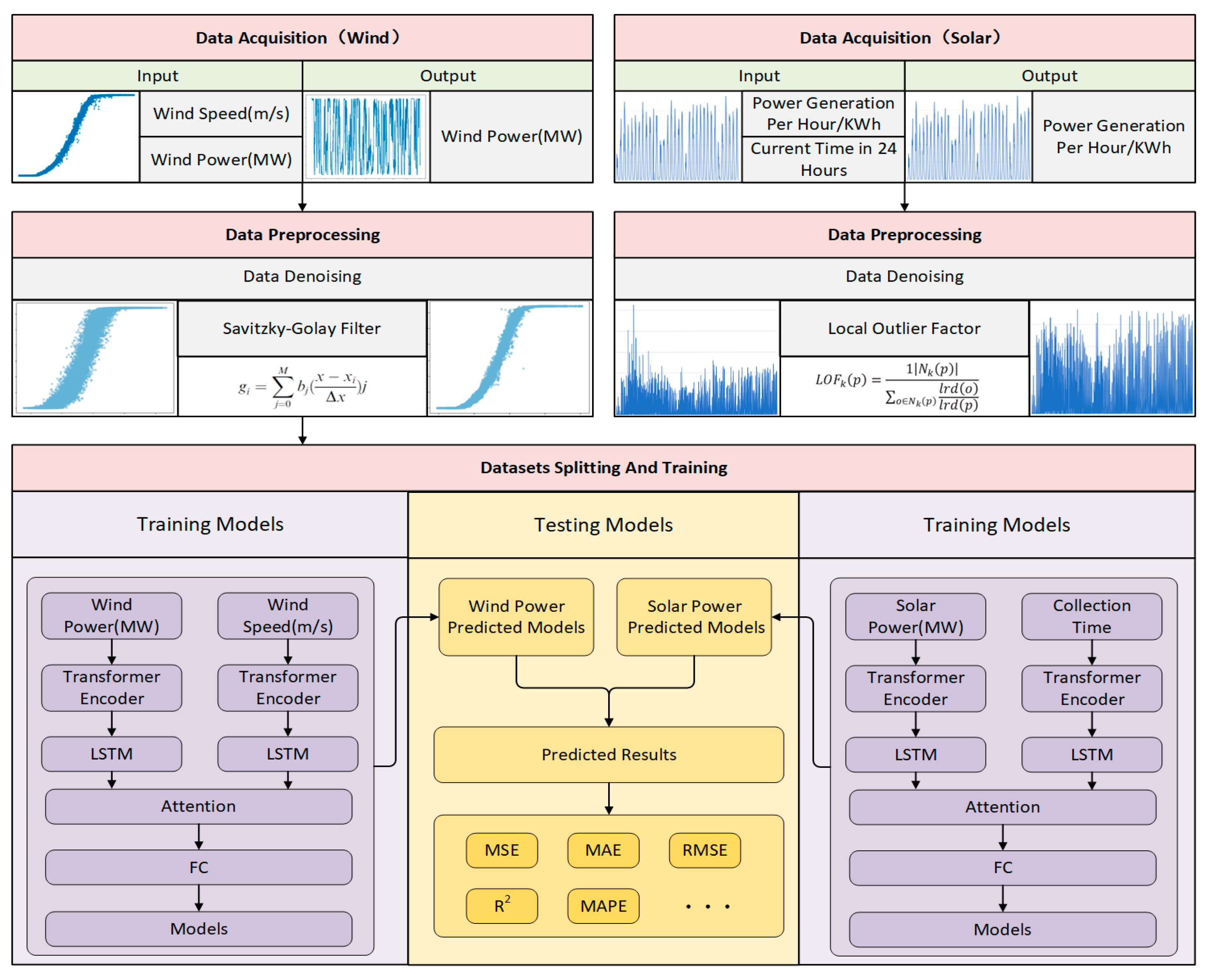
This section provides a detailed introduction to the power forecasting process for wind and solar power. The framework of the proposed method is presented in Figure 1. Firstly, we provided a detailed description of the data acquisition and preprocessing procedures for wind and solar energy data, establishing the input and output components of the data. Subsequently, we introduced two data denoising and filtering methods, namely the Savitzky–Golay (SG) filter and Local Outlier Factor (LOF) filter, to effectively reduce noise and outliers in the data. Next, we explained how the processed dataset was partitioned into training, validation, and test sets to prepare for model training and evaluation. Finally, we expounded on the network architecture of the proposed deep learning model, SL-Transformer, and outlined the evaluation and comparison methodology for experimental results among different algorithms.
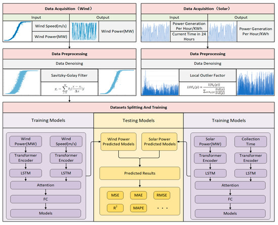
Figure 1.
The framework of SL-Transformer.
2.1. Data Acquisition
The study data come from one wind farm for one year and five photovoltaic farms for four months. Wind data include wind speed and power generation. Pv data include solar power generation and generation records.
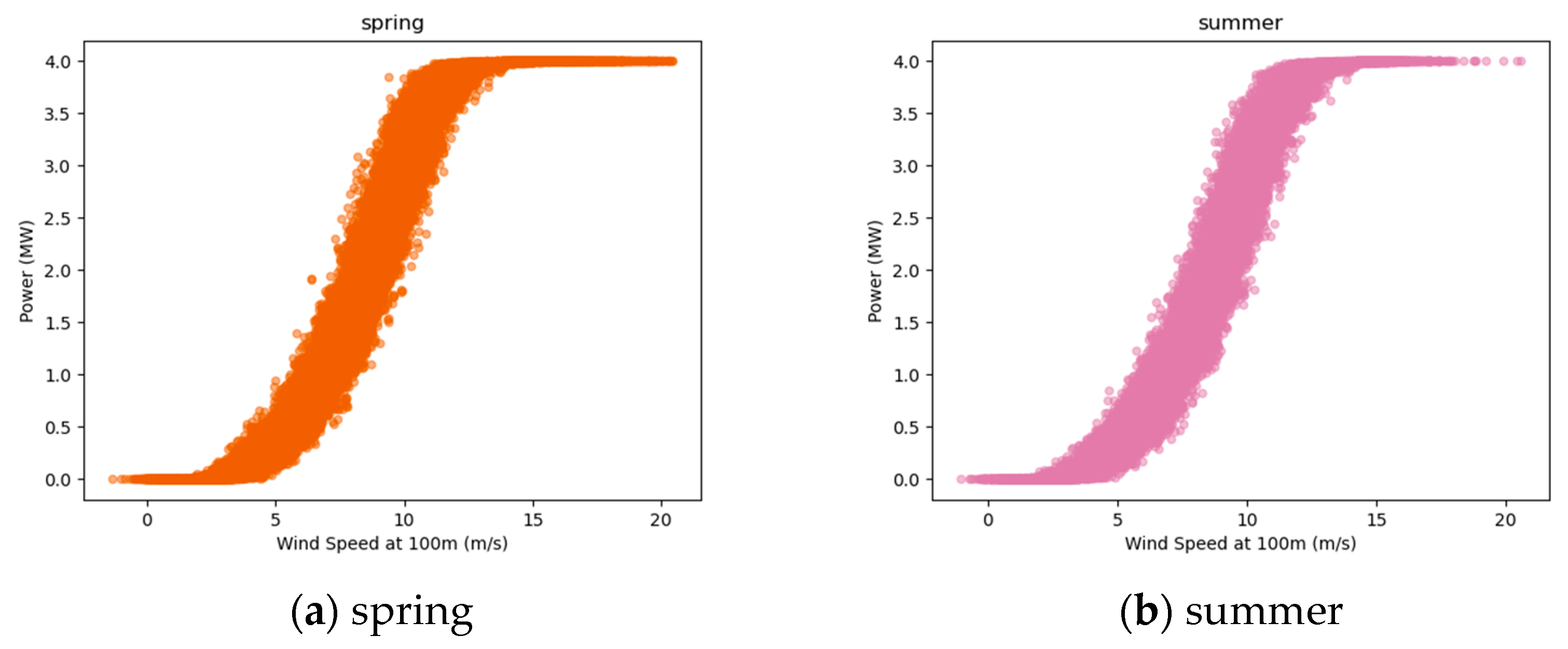
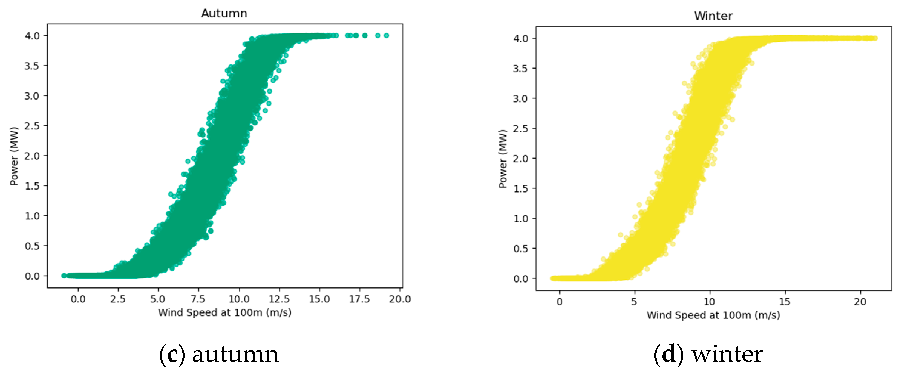
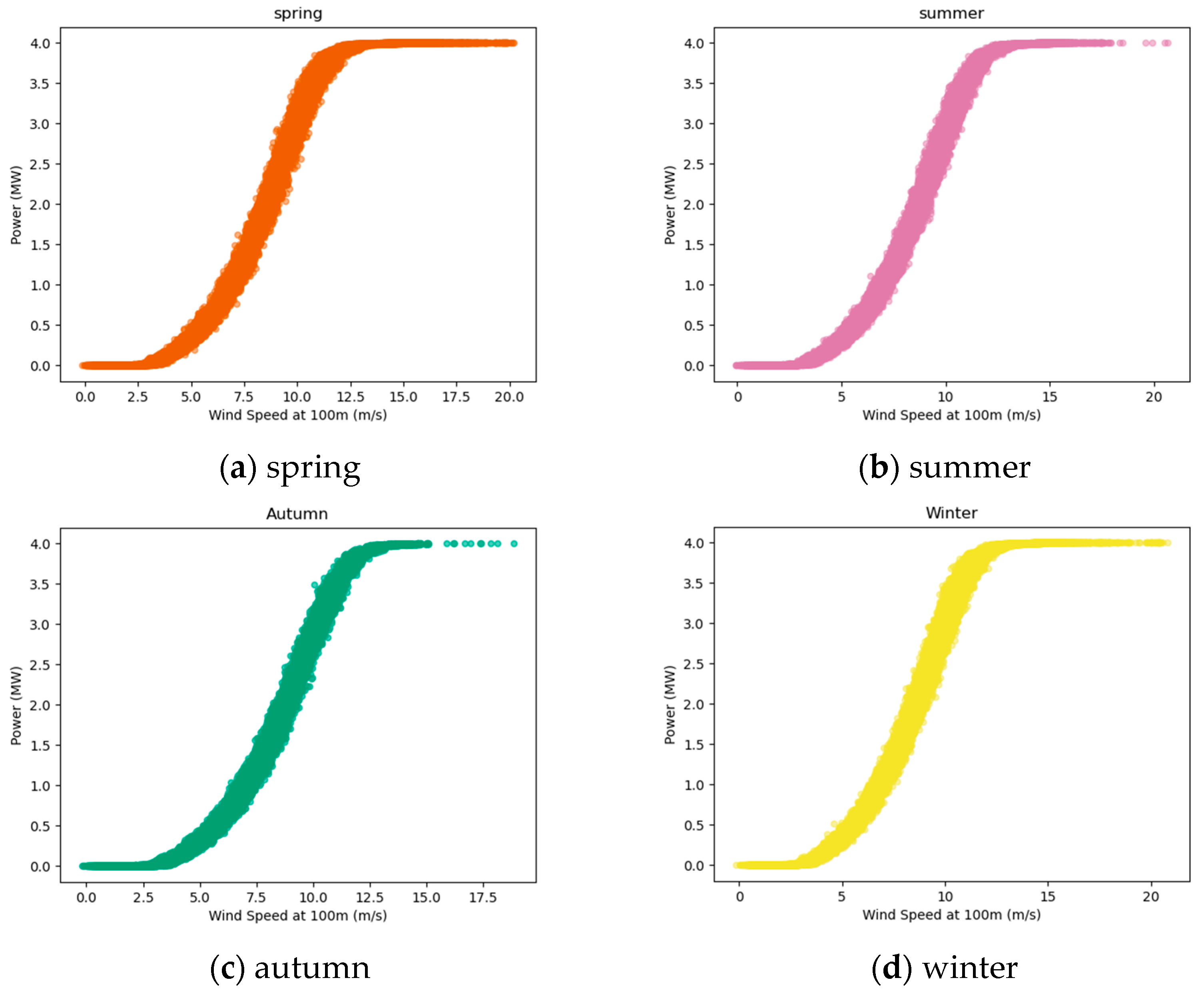
Figure 2 shows the scatter plot of wind speed and wind power generation in four seasons. The main range of wind speed data is between 3.08 and 14.24 m/s, while the corresponding wind power generation data mainly ranges from 0.02 to 4.00 MW. From the figure, it is evident that there is an overall upward trend in wind power generation with increasing wind speed, indicating a positive correlation between these two variables. Specifically, at lower wind speeds (3–6 m/s), the power generation remains at a lower level, reflecting the start-up phase of the wind turbines. As wind speed increases to around 12 m/s, power generation reaches its peak. Subsequently, with further increases in wind speed, wind turbines may limit power output or shut down due to safety considerations, resulting in stable power generation levels. This figure clearly demonstrates the impact of wind speed variations on wind power generation, providing a crucial foundation for establishing correlated models between wind speed and power generation. Consequently, this research contributes to wind power forecasting and management in wind farms.
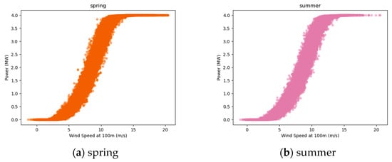
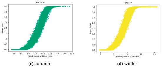
Figure 2.
Wind speed–power generation for four seasons.
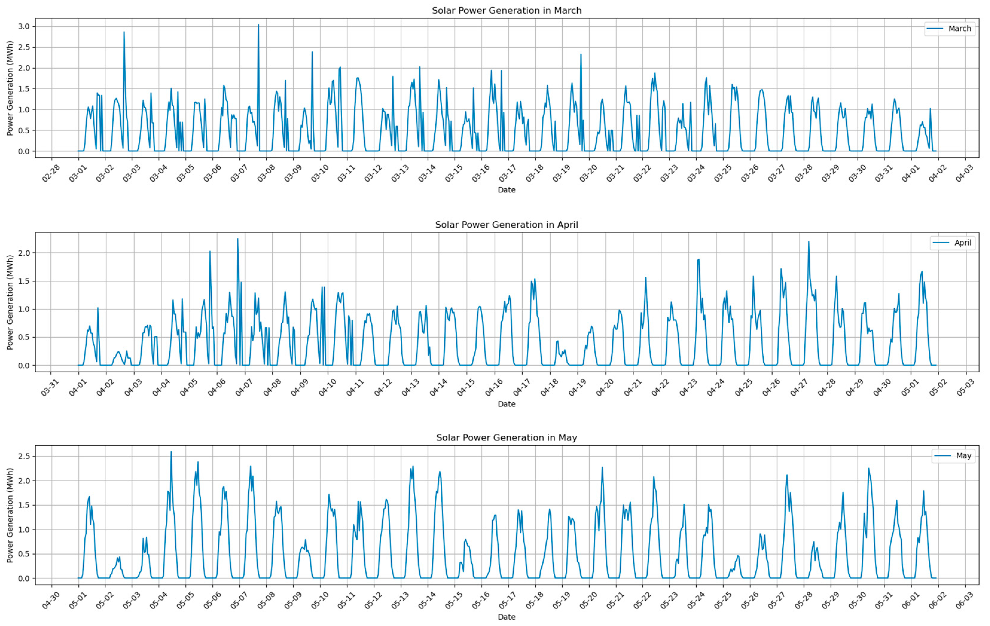
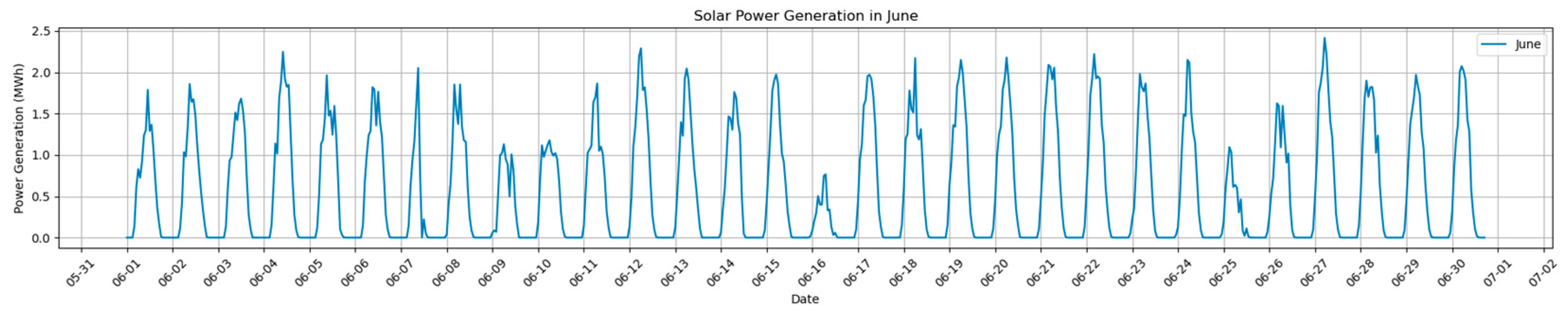
The data presented in Figure 3 encompasses the power generation of a specific photovoltaic site over a span of four months. The principal variables include the hour of the day to which a given record belongs and the corresponding power generation for that hour, measured in kilowatt-hours (kWh). The data reveal a distinct cyclic pattern in photovoltaic power generation: daily generation initiates an ascent after dawn, reaches its zenith in the afternoon, diminishes in the evening, and essentially tapers to zero during the night. The power generation curves for each day exhibit a high degree of similarity. Noteworthy patterns also emerge across different dates, potentially correlated with weather conditions; power generation decreases overall on overcast or rainy days. Furthermore, variations in power generation occur across different months due to varying solar angles and radiation intensities. The data exhibit favorable quality with continuity and integrity, devoid of conspicuous gaps. However, certain data points display anomalies, necessitating the application of filtering techniques for data refinement, ultimately culminating in power generation prediction employing time series models.
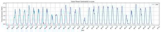
Figure 3.
Hourly solar energy generation over a four-month period.
2.2. Data Processing
Performing appropriate data preprocessing after obtaining raw data is a crucial step to enhance prediction outcomes. Both wind speed and solar data collected in this study contain outlier data points, which, if used directly, would diminish the accuracy of prediction models. Therefore, it is imperative to conduct filtering procedures to eliminate anomalies.
SG filter is applied for the wind speed data; the method constitutes a general approach for data smoothing, applicable to various types of data, including time series and image data. The fundamental idea underlying this technique involves local polynomial fitting to mitigate noise, effectively preserving the essential components of the data. For the time series the general polynomial fit form is as follows, where represents the order of the polynomial,
a localized region of length is selected, where is an odd number. This localized region encompasses a total of M data points, ranging from to . The coefficients of the polynomial fit are determined using the least squares method within this localized region. Assuming a polynomial fit of order , the objective of the fitting process is to determine coefficients , such that the residual sum of squares between the fitted polynomial and the local data points is minimized. The formula for calculating the residual sum of squares is as follows:
represents the value of the fitted polynomial at position . Within each localized region, the polynomial fitting function obtained by solving the least squares problem is evaluated at the position of the central data point , denoted as and this value is utilized as the smoothed signal value in place of the original signal .
By applying the Savitzky–Golay (SG) filter to the wind speed data, we effectively mitigated the noise and fluctuations inherent in the wind speed sensor readings. The filter’s smoothing operation preserves the essential features of the speed profile while eliminating short-term variations. This is evident through a comparison between wind speed and wind power generation, as depicted in Figure 4. After the application of the SG filter, we observe an augmented correlation between wind speed and wind power generation, indicative of the successful suppression of spurious oscillations and noise present in the original wind speed readings. This refinement enhances the reliability of the wind speed data, thereby contributing to a more dependable and efficient prediction of wind power output.
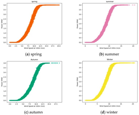
Figure 4.
Wind speed–power generation after filtering using the SG filter.
For solar power data, anomalies are directly removed during the deep night period (e.g., 2 h after sunset to 2 h before sunrise). At other times, the LOF filter is used to detect and adjust anomalous values. The LOF algorithm determines the abnormality of a data point based on the density relationship between the data point and its neighboring data points. In the experiment, to capture the daily periodicity of the data, the number of neighbors in the LOF algorithm was set to 24. The absolute distance between distinct points and is provided by
for a data point , compute its distance from all other data points in the dataset. Sort these distances and identify the -th smallest distance, which is termed the -distance of . The k-reachable distance of data point with respect to is defined as
and local reachability density () of an individual point is provided by
the calculation of the Local Outlier Factor is the central step of the LOF algorithm. It measures the relative density of a data point in comparison to its neighboring data points, thereby determining whether the data point is an outlier. When the LOF score is significantly greater than 1, it suggests that the data point might be an anomaly. The computation formula is as follows:
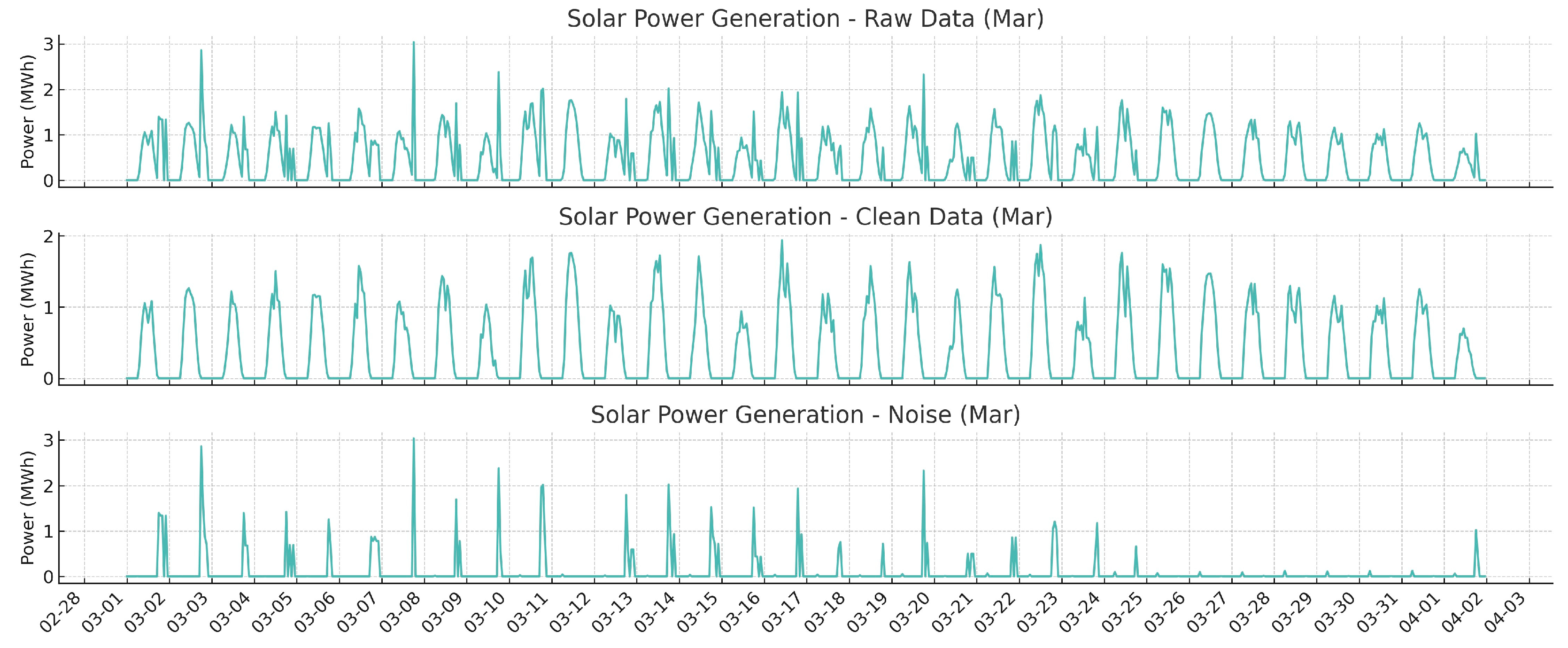
Figure 5 stands as a clear illustration of the LOF filter’s effectiveness, showcasing the solar power generation data for March both prior to and subsequent to the LOF filter’s application and delineating the extraneous noise that was identified and removed. Initially, the dataset was compromised by irregularities, presumably the result of measurement inaccuracies or unrelated environmental factors. The LOF filter proves particularly proficient at identifying such localized discrepancies and excising them from the data. This is exemplified by the filter’s precise identification and removal of aberrant data on the evening of March 8th, as shown in the figure—a period inherently devoid of solar power generation. The application of the LOF filter yields a dataset that reflects a more consistent and smooth progression of solar power generation, effectively eliminating outliers and markedly reducing the data’s fluctuation. This refinement process not only purifies the dataset but also bolsters the reliability of subsequent forecasting models, thereby ensuring more precise solar energy predictions.
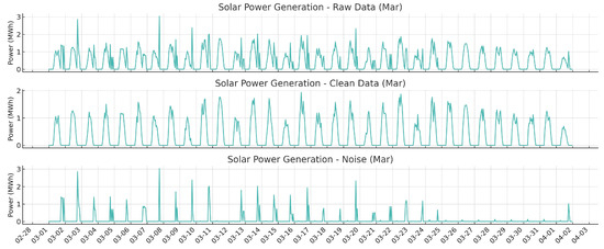
Figure 5.
Hourly solar power generation in March before and after applying the LOF filter.
2.3. Construction of the Predictive Model
This paper proposes a deep learning-based power prediction model for wind and solar power generation. The model employs an encoder–decoder framework, where the encoder component utilizes a Transformer architecture, the decoder part employs an LSTM structure, and an attention mechanism is utilized.
As depicted in Figure 1, for wind power prediction, the model’s input consists of wind power time series data and the corresponding wind speed data; for solar power generation prediction, the input includes solar power time series data and corresponding timestamp data. Both types of data are separately fed into the Transformer encoder for feature extraction. Our architecture adopts a standard Transformer block structure as defined by Vaswani [23]. We configure the encoder with three layers, each comprising a multi-head self-attention mechanism with three heads, where each head operates on one dimension. This multi-head attention architecture allows the model to focus on different positions of the input sequence, capturing a richer representation of the data. The self-attention mechanism of the encoder is complemented by position-wise feed-forward networks, which apply a linear transformation to each position separately and identically. Each of these networks consists of two linear transformations with a ReLU activation in between. The LSTM units receive the output from the Transformer encoder and handle the dynamic characteristics of the time series data.
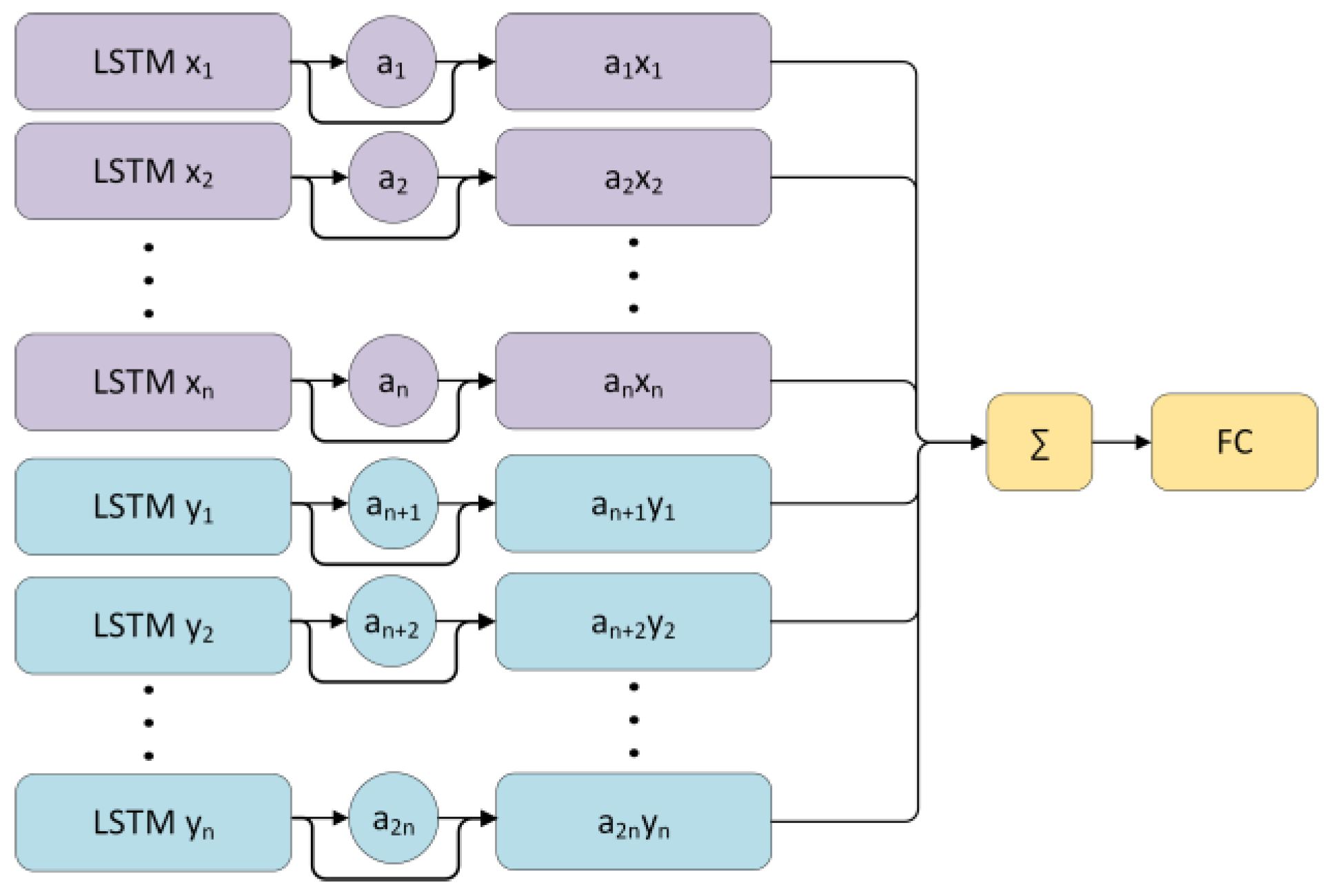
In Figure 6, the outcomes from these two LSTM units are conjoined through the attention mechanism, which subsequently conducts further processing of the LSTM unit outputs. This augmentation imparts to the model the adeptness to selectively attend to the salient constituents of the input data with respect to the desired output, thereby enhancing its discernment during the prognosticative procedure. The fully connected (FC) layer amalgamates the weighted features from the attention module, furnishing the model with a mapping from these features to the prediction of solar power generation. This accomplishes the transition from a high-dimensional feature space to a singular continuous output value, thereby defining decision boundaries based on input features and ultimately yielding solar power prediction outcomes.
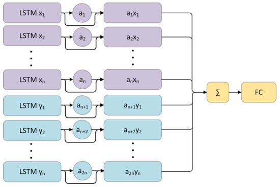
Figure 6.
The structure of attention mechanism.
In the outlined methodology, a comprehensive depiction has been presented regarding the various constituent elements of the model, encompassing tasks ranging from data preprocessing and feature extraction to time series modeling, culminating in the eventual generation of predictive output. To validate the effectiveness and performance of the model, the forthcoming section will meticulously detail the experimental configuration, dataset characteristics, evaluation metrics, and the comparative outcomes against existing methodologies.
3. Experiment
To evaluate the predictive performance of our model, we conducted a series of experiments. As shown in Figure 4 and Figure 5, the wind data and photovoltaic data we used have been presented in detail. For the partitioning of the dataset, we adopted an 8:2 ratio, where 80% of the data is used as a training set to train the model parameters, and the remaining 20% is used as a test set to evaluate the model’s performance on unseen data. Next, we describe in detail the setup of the experiment, the evaluation metrics, and the predictions of the model.
3.1. Data Description
In the experiments, the solar energy data primarily originated from real-time records at a photovoltaic power station, spanning four months with an hourly sampling interval. On the other hand, the wind energy data were derived from a year’s worth of power generation at a wind farm, including wind energy output and corresponding wind speed information, with a sampling interval of five minutes.
To ensure the reliability of our experimental results, we undertook a series of data preprocessing steps, such as outlier removal and data normalization. These pivotal procedures guarantee that the model receives high-quality data during both the training and testing phases, thereby enhancing the accuracy of predictions.
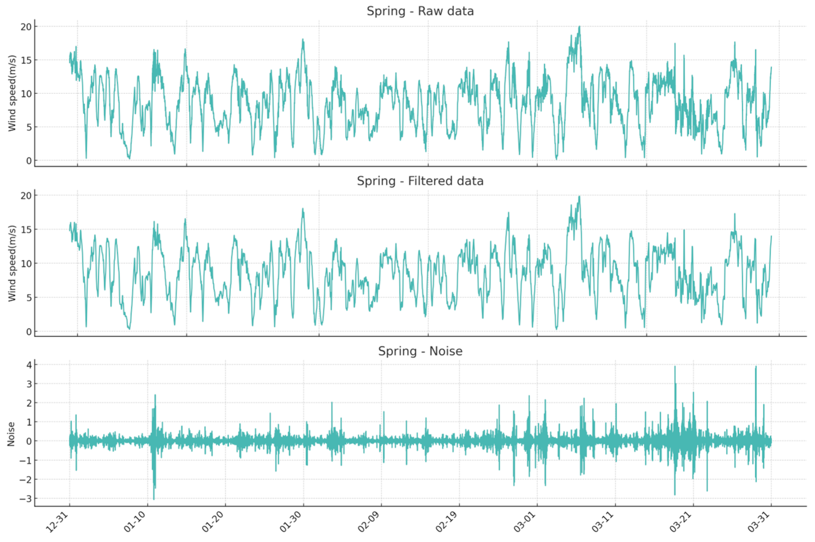
Figure 5 provides a detailed depiction of the preprocessing results for the solar energy data, while Figure 7 presents the spring wind speed data before and after noise reduction via the application of the SG filter. The raw data depicted in the figure exhibit a degree of volatility and irregular peaks, which can likely be attributed to sensor noise or environmental disturbances. Such noise can obfuscate the true pattern of wind speed and consequently blur its correlation with power generation.
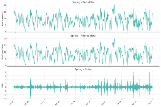
Figure 7.
Wind speed in spring at five-minute intervals before and after applying the SG filter.
During the experimental phase, the parameters of the SG filter were meticulously adjusted according to the characteristics of our dataset. A strategy was adopted to traverse the data with a moving window, fitting polynomials within each window to the data and then generating a smoothed value for each point. After extensive experimentation, a window length of 60 was selected for this study. The SG filter effectively eliminated noise from the wind speed data, more accurately reflecting the true dynamics of the wind speed.
The efficacy of this noise reduction is further illustrated in Figure 2 and Figure 4, which show the relationship between wind speed and power generation before and after denoising, respectively. Prior to the application of the SG filter, the correlation between wind speed and power generation was less apparent due to the noise. However, after filtering, the wind speed data align more closely with the power output, indicating a cleaner and more reliable dataset that can be used for more accurate wind power forecasting.
Through data preprocessing, the quality of wind and solar power data has been enhanced. This not only bolsters the credibility of the data but also furnishes subsequent modeling and analysis with a more uniform and continuous data source. The reduction in data anomalies and noise also mitigates the risk of model overfitting.
3.2. Green Energy Power Prediction
In this section, we present the results of wind power and solar power predictions. By utilizing the model depicted in Figure 1, we predict the electricity generation of wind and solar energy and then compare these predictions with the actual data to evaluate the model’s predictive performance.
3.2.1. Wind Power Prediction Results
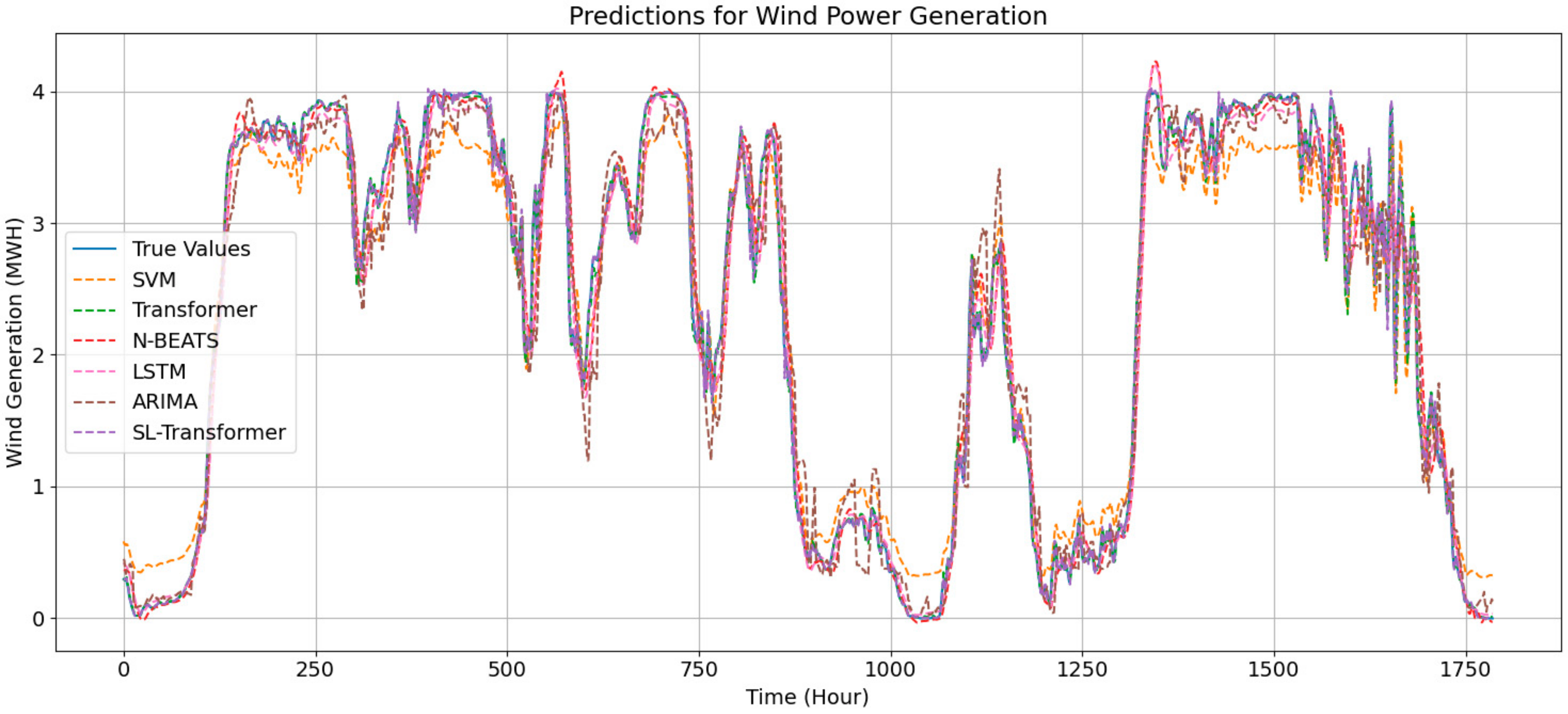
As depicted in Figure 8, the prediction outcomes for wind power generation are presented. The figure contrasts the wind power generation forecasts produced by various models with the actual power output. The trends of predicted and observed values are distinctly discernible within the illustration. Overall, the performance of all predictive models appears commendable, potentially attributable to effective data preprocessing. For a more nuanced comparison of model performance, one should refer to the evaluation metrics provided in Table 1. The formulas used for calculating these metrics are as follows:
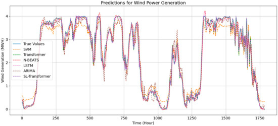
Figure 8.
Prediction results of wind power generation from different models.

Table 1.
Evaluation metrics for wind power generation prediction results.
From Table 1, various evaluation metrics gauge the prediction results of wind power generation for different models. The metrics include Mean Square Error (MSE), Mean Absolute Error (MAE), Root Mean Square Error (RMSE), Coefficient of determination (), and Symmetric Mean Absolute Percentage Error (SMAPE). Among the models evaluated for wind power prediction, the proposed SL-Transformer demonstrates the highest accuracy, as indicated by its near-perfect and SMAPE value. The LSTM and Transformer models demonstrate comparable performance, closely followed by NBEATS, the values of each model are approximately around 0.97, with the SVM slightly lagging behind the others. The proposed SL-Transformer, however, achieves an value of 0.9989, and its SMAPE is only 5.8507, demonstrating excellent performance in wind power forecasting tasks. The efficacy of this method is further validated by the empirical results.
3.2.2. Solar Power Prediction Results
Following the wind power forecasting, Figure 9 offers a visual representation of the solar power generation predictions. Similar to the wind power results, a consistent trend is observed between the predicted and actual solar energy outputs.
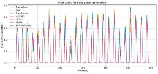
Figure 9.
Prediction results of solar power generation from different models.
Table 2 presents a range of evaluation metrics showcasing the efficacy of various models in solar energy forecasting. The proposed SL-Transformer model markedly surpasses its counterparts with an value of 0.9674 and an SMAPE value of 4.2156, indicating a closer alignment with the actual values. In contrast, other models hover around an value of approximately 0.92, with SMAPE values exceeding 10%, signifying that the proposed model demonstrates superior performance in predicting solar energy compared to the other models.
Table 2.
Evaluation metrics for solar power generation prediction results.
Although the proposed model exhibits exceptional predictive performance, in order to investigate the balance between performance improvement and computational complexity, in Table 3, we demonstrate the time consumed for prediction by the SL-Transformer in comparison with other models. Table 3 reveals that traditional algorithms like SVM, NBEATS, and ARIMA achieve rapid computation in both solar and wind forecasting scenarios. Conversely, the deep learning models, namely LSTM, Transformer, and SL-Transformer, require a longer processing time. However, given the sampling intervals of 5 min for wind and 1 h for solar predictions in our study, a marginal increase in computation time—measured in mere seconds—is outweighed by the benefit of higher prediction accuracy. Thus, the additional computational expense is warranted to achieve superior predictive performance.
Table 3.
Comparative analysis of prediction time across models (in seconds).
4. Discussion
Forecasting power generation from wind and solar energy sources is crucial in our journey toward sustainable energy practices. This study presents the SL-Transformer model, emphasizing its capability in time-series power forecasting. Comparative experiments with other leading deep learning models highlight the SL-Transformer’s exceptional prowess in forecasting. Notably, its value verges on perfection, particularly in wind power predictions. The experimental findings indicate that the suggested model adeptly captures the time-based relationships present in the data. Moreover, we integrate a pair of filtering techniques, effectively purging the wind and solar data of irrelevant noise and outliers. This process has endowed the models with a higher caliber of input data, consequently elevating the accuracy of the predictive outcomes.
However, while the results from the SL-Transformer are promising, this investigation is not devoid of limitations. The restricted span of solar data, limited to four months, might not encompass the full spectrum of seasonal intricacies, potentially compromising its forecasting efficacy in broader contexts. Additionally, when deployed in real-world scenarios, the model might confront uncharted challenges absent in the test dataset. Future endeavors should prioritize an expansion of the dataset in terms of duration and diversity. There is also merit in considering the incorporation of additional parameters to bolster predictive accuracy. Exploring ensemble methods that combine the advantages of various models could offer a promising direction for future research.
5. Conclusions
In light of the increasing emphasis on green energy in contemporary society, this paper introduces a novel approach to forecasting power generation from renewable sources, particularly wind and solar energy. The SL-Transformer model, as presented in this study, has demonstrated exceptional efficacy in time-series power forecasting. With an value of 0.9989 and a significantly low SMAPE of 5.8507%, its wind power prediction is almost flawless. While the solar power prediction result stands at 0.9674, a SMAPE of 4.2156%, it still represents a 15% improvement over other algorithms. The forecasting results for both types of green energy surpassed other prediction algorithms, suggesting that the proposed method exhibits robustness in recognizing time-dependent relationships within the data. Additionally, a unique data preprocessing method has been utilized to eliminate anomalies in wind speed and photovoltaic data, ensuring that maximum relevant information is extracted and retained, which has further contributed to enhancing the accuracy of subsequent power predictions.
Nevertheless, this study is not without its limitations, primarily concerning the restricted scope of the solar data. Such constraints might lead to overlooking potential seasonal variations, limiting the broader applicability of the model. The potential challenges that could arise in real-world applications further underscore the need for caution. Moving forward, it becomes imperative to expand the diversity of our experimental dataset both temporally and spatially. Moreover, we intend to incorporate data from a wider variety of green energy sources to test our methodology. Such expansions will not only bolster the model’s generalizability but also refine its forecasting precision.
Author Contributions
Conceptualization, J.Z., Z.A., Y.G. and Z.Z.; methodology, X.Z., Q.G. and Z.L.; validation, J.Z., J.S. and Z.L.; formal analysis, Z.Z. and X.Z.; investigation, X.Z., Q.G. and Y.G.; resources, J.Z., Z.L. and Y.G.; data curation, Z.A. and Z.L.; writing—original draft preparation, J.Z., Z.Z., Z.A. and Y.G.; writing—review and editing, X.Z., Q.G. and J.S.; visualization, Z.L., Z.A. and Y.G; supervision, Y.G.; project administration, J.Z.; funding acquisition, Y.G. All authors have read and agreed to the published version of the manuscript.
Funding
This research was funded by the Shenzhen International Cooperation Project, grant number GJHZ20210705141401005; Science and Technology project of Tianjin, China, grant number 22YFYSHZ00330; and Shenzhen Science and Technology Plan, Sustainable Development Technology Special Project (Dual-Carbon Special Project), grant number KCXST20221021111402006.
Data Availability Statement
Data are not available due to privacy.
Acknowledgments
This research is supported by the “Nanling Team Project” of Shaoguan City. In addition, the authors would like to thank the editor and the reviewers for their constructive comments.
Conflicts of Interest
Author Jian Zhu, Zhiyuan Zhao, Xiaoran Zheng, Qingwu Guo, Zhikai Li, Jianling Sun are employed by the company SPIC Integrated Smart Energy Technology Co., Ltd. The remaining authors declare that the research was conducted in the absence of any commercial or financial relationships that could be construed as a potential conflict of interest.
References
- Zheng, J.; Du, J.; Wang, B.; Klemeš, J.J.; Liao, Q.; Liang, Y. A hybrid framework for forecasting power generation of multiple renewable energy sources. Renew. Sustain. Energy Rev. 2023, 172, 113046. [Google Scholar] [CrossRef]
- Markovics, D.; Mayer, M.J. Comparison of machine learning methods for photovoltaic power forecasting based on numerical weather prediction. Renew. Sustain. Energy Rev. 2022, 161, 112364. [Google Scholar] [CrossRef]
- Yang, Z.; Hu, T.; Zhu, J.; Shang, W.; Guo, Y.; Foley, A. Hierarchical High-Resolution Load Forecasting for Electric Vehicle Charging: A Deep Learning Approach. IEEE J. Emerg. Sel. Top. Ind. Electron. 2022, 4, 118–127. [Google Scholar] [CrossRef]
- Li, Y.; Wang, R.; Li, Y.; Zhang, M.; Long, C. Wind power forecasting considering data privacy protection: A federated deep reinforcement learning approach. Appl. Energy 2023, 329, 120291. [Google Scholar] [CrossRef]
- Zhang, L.; Hu, T.; Zhang, L.; Yang, Z.; McLoone, S.; Menhas, M.I.; Guo, Y. A novel dynamic opposite learning enhanced Jaya optimization method for high efficiency plate–fin heat exchanger design optimization. Eng. Appl. Artif. Intell. 2023, 119, 105778. [Google Scholar] [CrossRef]
- Ma, Z.; Mei, G. A hybrid attention-based deep learning approach for wind power prediction. Appl. Energy 2022, 323, 119608. [Google Scholar] [CrossRef]
- Yaprakdal, F.; Yılmaz, M.B.; Baysal, M.; Anvari-Moghaddam, A. A deep neural network-assisted approach to enhance short-term optimal operational scheduling of a microgrid. Sustainability 2020, 12, 1653. [Google Scholar] [CrossRef]
- Moradzadeh, A.; Moayyed, H.; Zakeri, S.; Mohammadi-Ivatloo, B.; Aguiar, A.P. Deep learning-assisted short-term load forecasting for sustainable management of energy in microgrid. Inventions 2021, 6, 15. [Google Scholar] [CrossRef]
- Tian, C.; Niu, T.; Wei, W. Developing a wind power forecasting system based on deep learning with attention mechanism. Energy 2022, 257, 124750. [Google Scholar] [CrossRef]
- Tawn, R.; Browell, J. A review of very short-term wind and solar power forecasting. Renew. Sustain. Energy Rev. 2022, 153, 111758. [Google Scholar] [CrossRef]
- Akbal, Y.; Ünlü, K.D. A univariate time series methodology based on sequence-to-sequence learning for short to midterm wind power production. Renew. Energy 2022, 200, 832–844. [Google Scholar] [CrossRef]
- Afrasiabi, M.; Mohammadi, M.; Rastegar, M.; Stankovic, L.; Afrasiabi, S.; Khazaei, M. Deep-based conditional probability density function forecasting of residential loads. IEEE Trans. Smart Grid 2020, 11, 3646–3657. [Google Scholar] [CrossRef]
- Islam, M.K.; Hassan, N.M.S.; Rasul, M.G.; Emami, K.; Chowdhury, A.A. Forecasting of Solar and Wind Resources for Power Generation. Energies 2023, 16, 6247. [Google Scholar] [CrossRef]
- Yang, Z.; Mourshed, M.; Liu, K.; Xu, X.; Feng, S. A novel competitive swarm optimized RBF neural network model for short-term solar power generation forecasting. Neurocomputing 2020, 397, 415–421. [Google Scholar] [CrossRef]
- Lim, S.C.; Huh, J.H.; Hong, S.H.; Park, C.Y.; Kim, J.C. Solar Power Forecasting Using CNN-LSTM Hybrid Model. Energies 2022, 15, 8233. [Google Scholar] [CrossRef]
- Mehta, Y.; Xu, R.; Lim, B.; Wu, J.; Gao, J. A Review for Green Energy Machine Learning and AI Services. Energies 2023, 16, 5718. [Google Scholar] [CrossRef]
- Liu, Z.; Liu, Z.; Liu, M.; Wang, J. Optimization of flow shop scheduling in precast concrete component production via mixed-integer linear programming. Adv. Civ. Eng. 2021, 2021, 1–14. [Google Scholar] [CrossRef]
- Wu, Y.K.; Huang, C.L.; Phan, Q.T.; Li, Y.Y. Completed review of various solar power forecasting techniques considering different viewpoints. Energies 2022, 15, 3320. [Google Scholar] [CrossRef]
- Al-qaness, M.A.; Ewees, A.A.; Fan, H.; Abualigah, L.; Abd Elaziz, M. Boosted ANFIS model using augmented marine predator algorithm with mutation operators for wind power forecasting. Appl. Energy 2022, 314, 118851. [Google Scholar] [CrossRef]
- Alassery, F.; Alzahrani, A.; Khan, A.I.; Irshad, K.; Islam, S. An artificial intelligence-based solar radiation prophesy model for green energy utilization in energy management system. Sustain. Energy Technol. Assess. 2022, 52, 102060. [Google Scholar] [CrossRef]
- Cheng, L.; An, Z.; Guo, Y.; Ren, M.; Yang, Z.; McLoone, S. MMFSL: A Novel Multimodal Few-Shot Learning Framework for Fault Diagnosis of Industrial Bearings. IEEE Trans. Instrum. Meas. 2023, 72, 1–13. [Google Scholar] [CrossRef]
- Haider, S.A.; Sajid, M.; Sajid, H.; Uddin, E.; Ayaz, Y. Deep learning and statistical methods for short-and long-term solar irradiance forecasting for Islamabad. Renew. Energy 2022, 198, 51–60. [Google Scholar] [CrossRef]
- Vaswani, A.; Shazeer, N.; Parmar, N.; Uszkoreit, J.; Jones, L.; Gomez, A.N.; Polosukhin, I. Attention is all you need. Adv. Neural Inf. Process. Syst. 2017, 30, 5998–6008. [Google Scholar]
- LeCun, Y.; Bengio, Y.; Hinton, G. Deep learning. Nature 2015, 521, 436–444. [Google Scholar] [CrossRef] [PubMed]
- Lv, S.X.; Wang, L. Deep learning combined wind speed forecasting with hybrid time series decomposition and multi-objective parameter optimization. Appl. Energy 2022, 311, 118674. [Google Scholar] [CrossRef]
- An, Z.; Cheng, L.; Guo, Y.; Ren, M.; Feng, W.; Sun, B.; Ling, J.; Chen, H.; Chen, W.; Luo, Y.; et al. A Novel Principal Component Analysis-Informer Model for Fault Prediction of Nuclear Valves. Machines 2022, 10, 240. [Google Scholar] [CrossRef]
- Mathew, A.; Amudha, P.; Sivakumari, S. Deep learning techniques: An overview. Adv. Mach. Learn. Technol. Appl. Proc. AMLTA 2020, 2021, 599–608. [Google Scholar]
- Wu, C.; Li, X.; Guo, Y.; Wang, J.; Ren, Z.; Wang, M.; Yang, Z. Natural language processing for smart construction: Current status and future directions. Autom. Constr. 2022, 134, 104059. [Google Scholar] [CrossRef]
- Tuerxun, W.; Xu, C.; Guo, H.; Guo, L.; Zeng, N.; Gao, Y. A wind power forecasting model using LSTM optimized by the modified bald eagle search algorithm. Energies 2022, 15, 2031. [Google Scholar] [CrossRef]
- Wang, Y.; Zou, R.; Liu, F.; Zhang, L.; Liu, Q. A review of wind speed and wind power forecasting with deep neural networks. Appl. Energy 2021, 304, 117766. [Google Scholar] [CrossRef]
- De Caro, F.; De Stefani, J.; Vaccaro, A.; Bontempi, G. DAFT-E: Feature-Based Multivariate and Multi-Step-Ahead Wind Power Forecasting. IEEE Trans. Sustain. Energy 2022, 13, 1199–1209. [Google Scholar] [CrossRef]
- Zhou, Y.; Wang, J.; Li, Z.; Lu, H. Short-term photovoltaic power forecasting based on signal decomposition and machine learning optimization. Energy Convers. Manag. 2022, 267, 115944. [Google Scholar] [CrossRef]
- Cui, W.; Wan, C.; Song, Y. Ensemble Deep Learning-Based Non-Crossing Quantile Regression for Nonparametric Probabilistic Forecasting of Wind Power Generation. IEEE Trans. Power Syst. 2023, 38, 3163–3178. [Google Scholar] [CrossRef]
- Wang, C.; Wang, Y.; Ding, Z.; Zheng, T.; Hu, J.; Zhang, K. A transformer-based method of multienergy load forecasting in integrated energy system. IEEE Trans. Smart Grid 2022, 13, 2703–2714. [Google Scholar] [CrossRef]
- Mancuso, P.; Piccialli, V.; Sudoso, A.M. A machine learning approach for forecasting hierarchical time series. Expert Syst. Appl. 2021, 182, 115102. [Google Scholar] [CrossRef]
- Brégère, M.; Huard, M. Online hierarchical forecasting for power consumption data. Int. J. Forecast. 2022, 38, 339–351. [Google Scholar] [CrossRef]
- Yang, H.; Cheng, Y.; Li, G. A denoising method for ship radiated noise based on Spearman variational mode decomposition, spatial-dependence recurrence sample entropy, improved wavelet threshold denoising, and Savitzky-Golay filter. Alex. Eng. J. 2021, 60, 3379–3400. [Google Scholar] [CrossRef]
- Li, H.; Ren, Z.; Xu, Y.; Li, W.; Hu, B. A Multi-Data Driven Hybrid Learning Method for Weekly Photovoltaic Power Scenario Forecast. IEEE Trans. Sustain. Energy 2022, 13, 91–100. [Google Scholar] [CrossRef]

Disclaimer/Publisher’s Note: The statements, opinions and data contained in all publications are solely those of the individual author(s) and contributor(s) and not of MDPI and/or the editor(s). MDPI and/or the editor(s) disclaim responsibility for any injury to people or property resulting from any ideas, methods, instructions or products referred to in the content. |
© 2023 by the authors. Licensee MDPI, Basel, Switzerland. This article is an open access article distributed under the terms and conditions of the Creative Commons Attribution (CC BY) license (https://creativecommons.org/licenses/by/4.0/).