
A New Methodology for Determination of Layered Injection Allocation in Highly Deviated Wells Drilled in Low-Permeability Reservoirs

Abstract
:1. Introduction
2. Geological Background
3. Sand Body Connectivity Evaluation
3.1. Identification of a Single Sand Body
3.1.1. Vertical Interface Characteristics and Stacking Patterns of Single Sand Body
- (1)
- Single-period channel vertical isolated type
- (2)
- Multiperiod channel vertical separation type
- (3)
- Multiperiod channel vertical superposition type
- (4)
- Multiperiod channel cutting and stacking type
3.1.2. Lateral Contact Relationship and Identification Mark of a Single Sand Body
- (1)
- Inter-bay contact
- (2)
- Levee contact
- (3)
- Side-cut contact
- (4)
- Substitutive contact
- (5)
- Docking contact
3.2. Single Sand Body Division Method
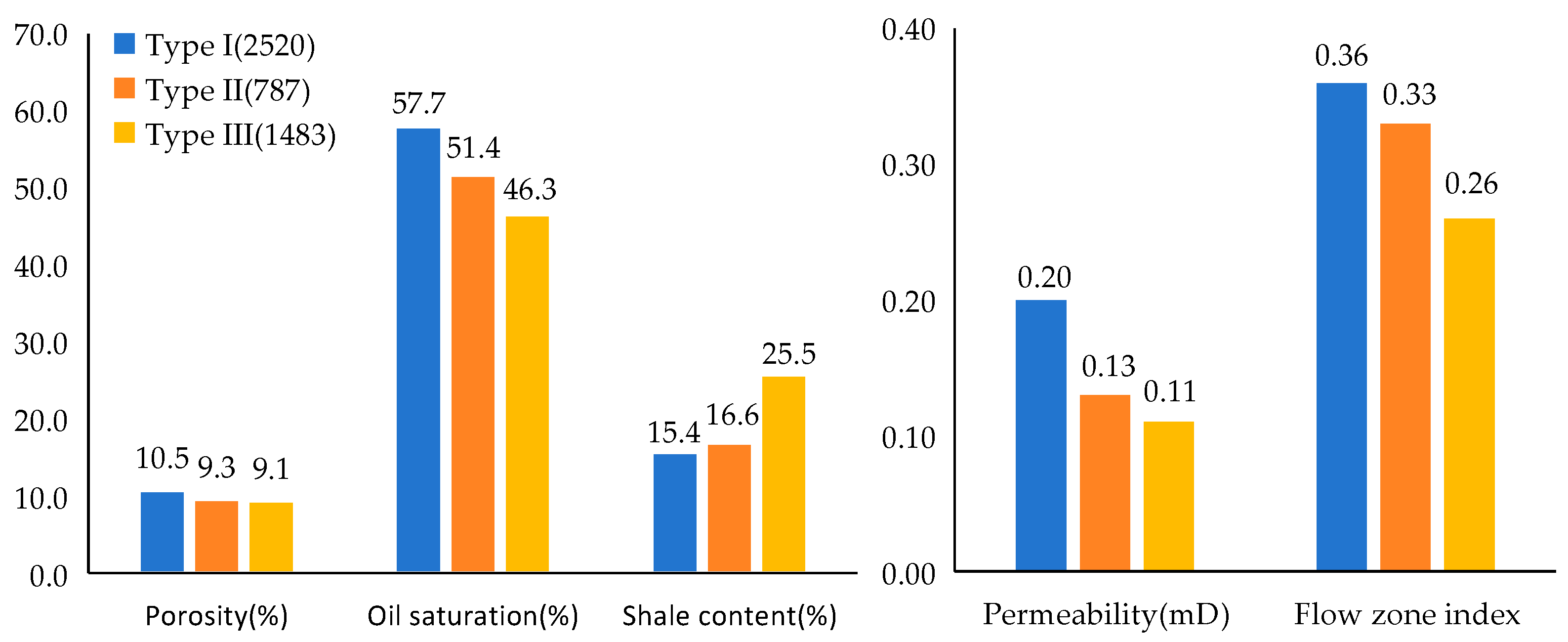
3.2.1. Flow Unit Division of Single Sand Body
3.2.2. Quantitative Prediction of a Single Sand Body Boundary
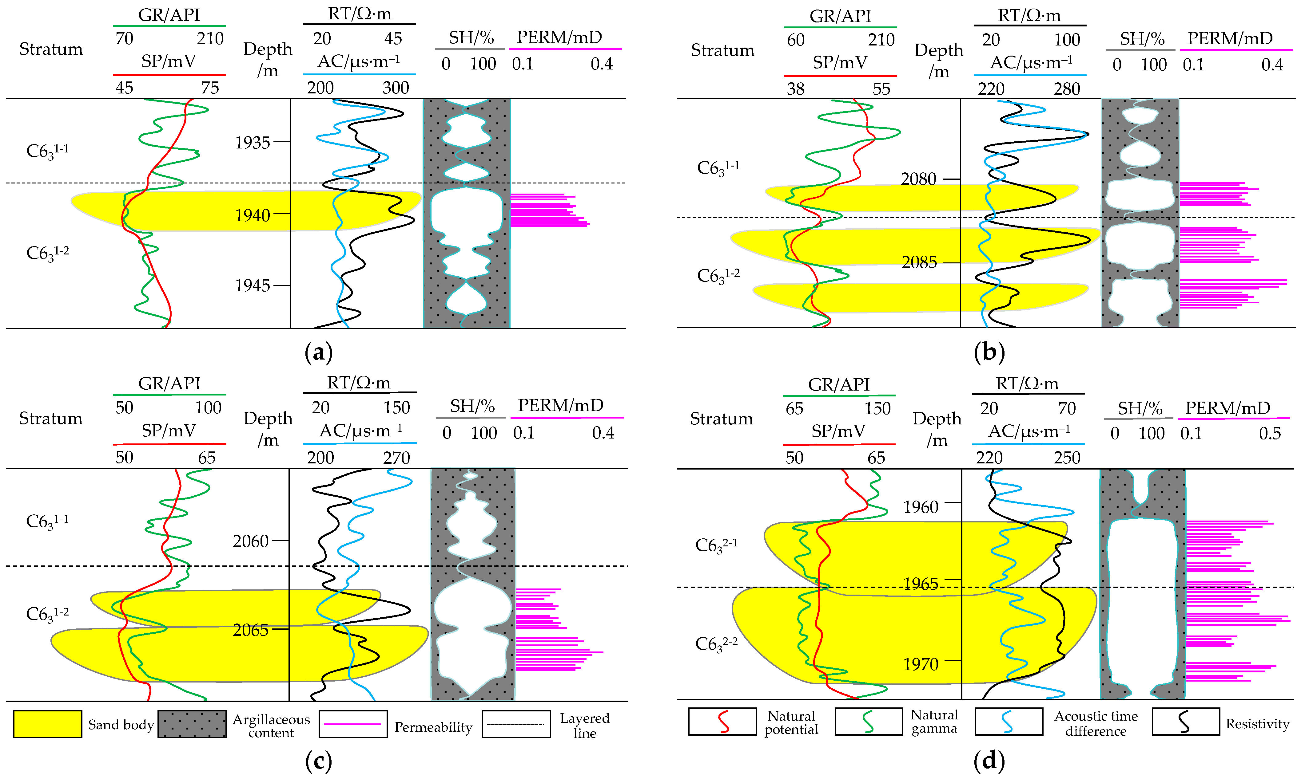
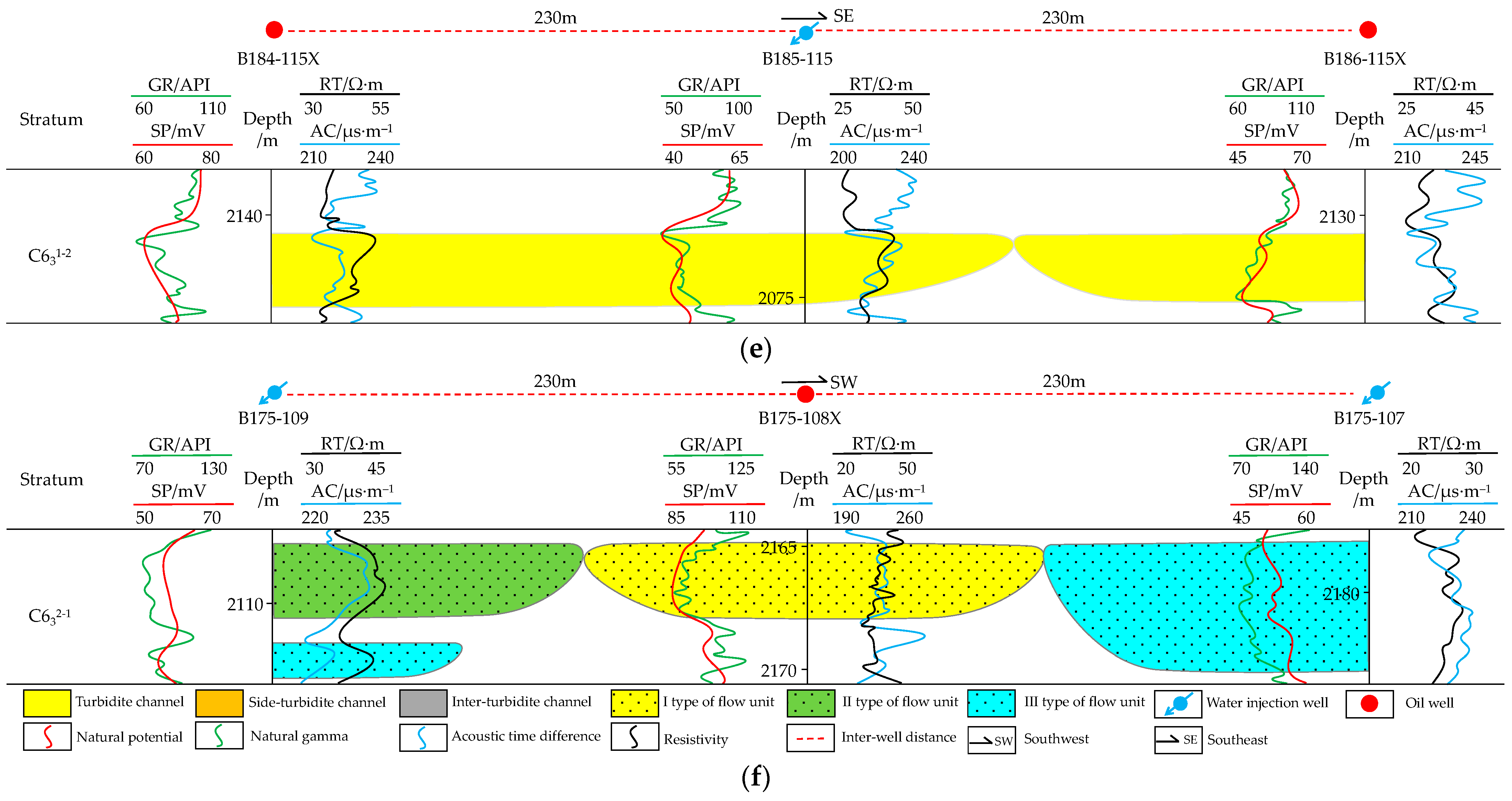
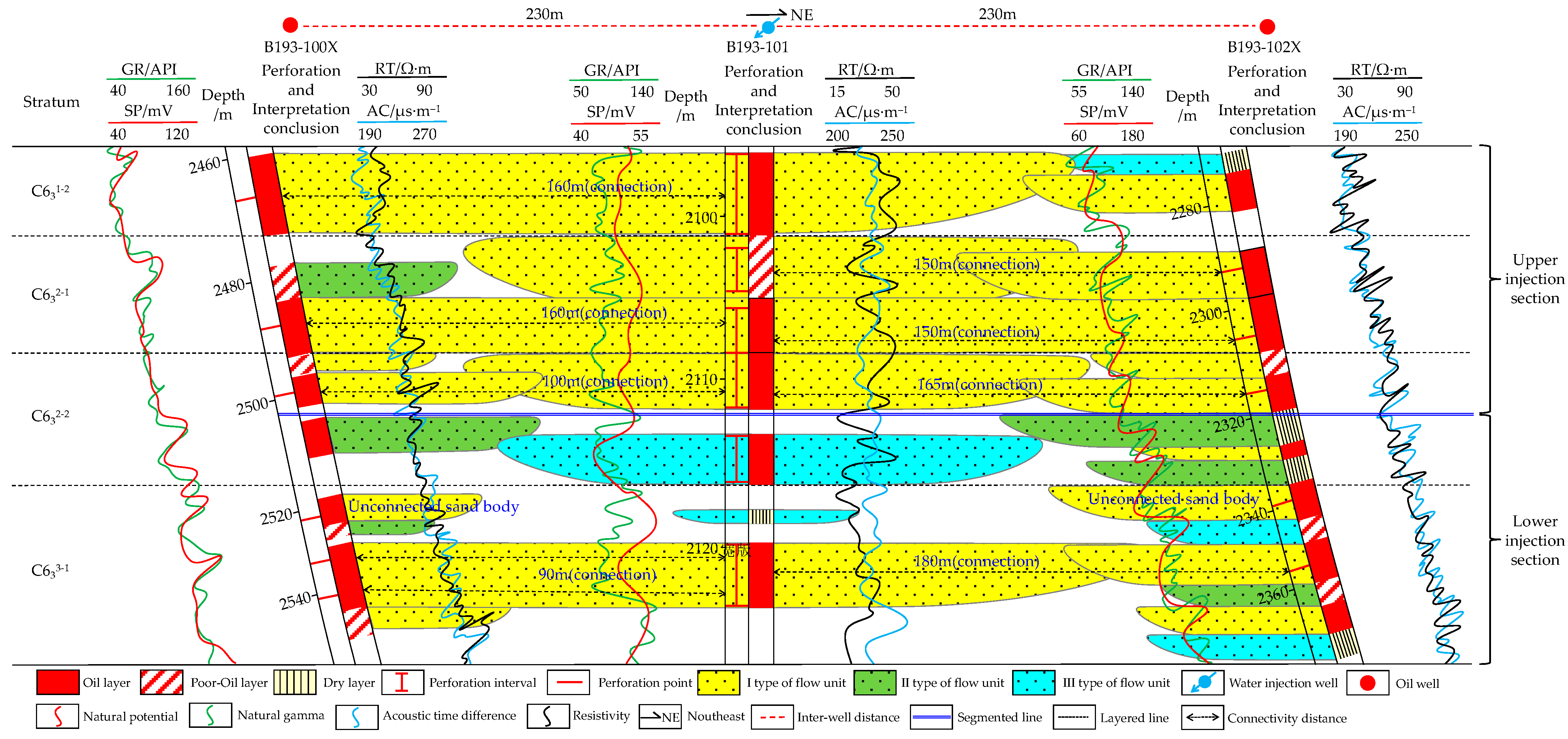
3.2.3. Example of the Flow Unit Correction and Single Sand Body Contact Relationship
3.3. Quantitative Evaluation of the Sand Body Connectivity
- (1)
- Connectivity coefficient
- (2)
- Transition coefficient
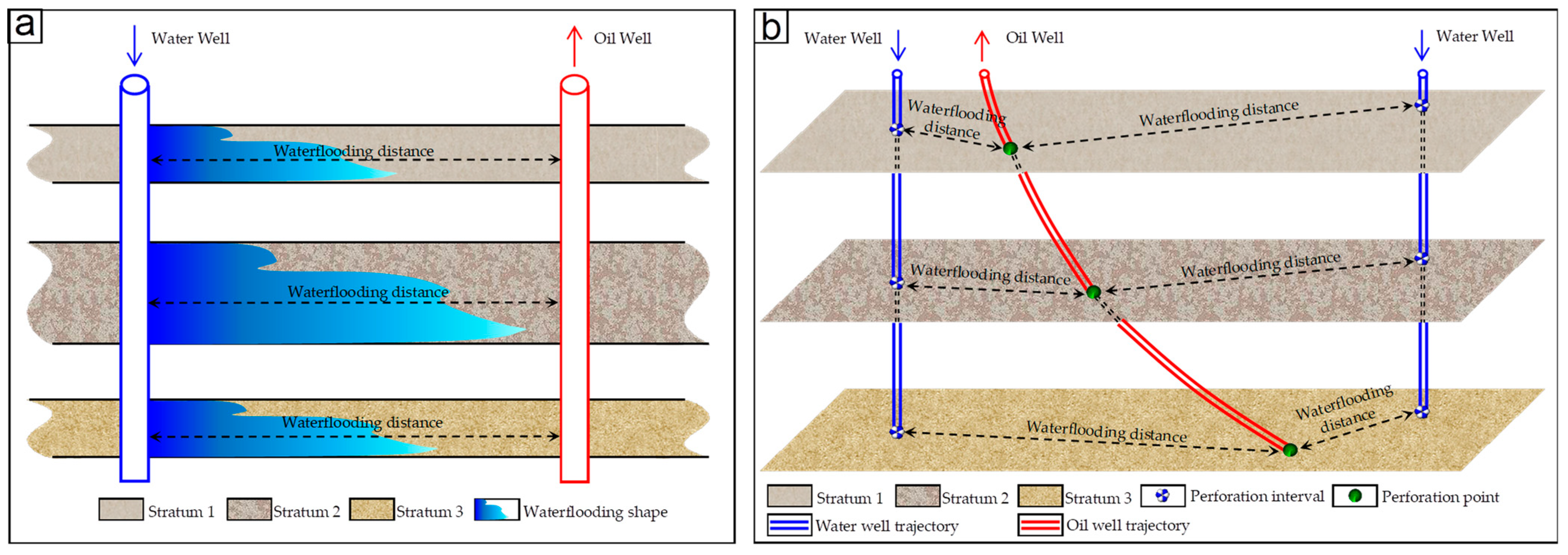
4. Calculation of Real Displacement Distance
5. Layered Injection Allocation Calculation Method
5.1. Layered Injection Allocation Calculation Formula
5.2. Calculation Example of Layered Injection Allocation in Highly Deviated Wells
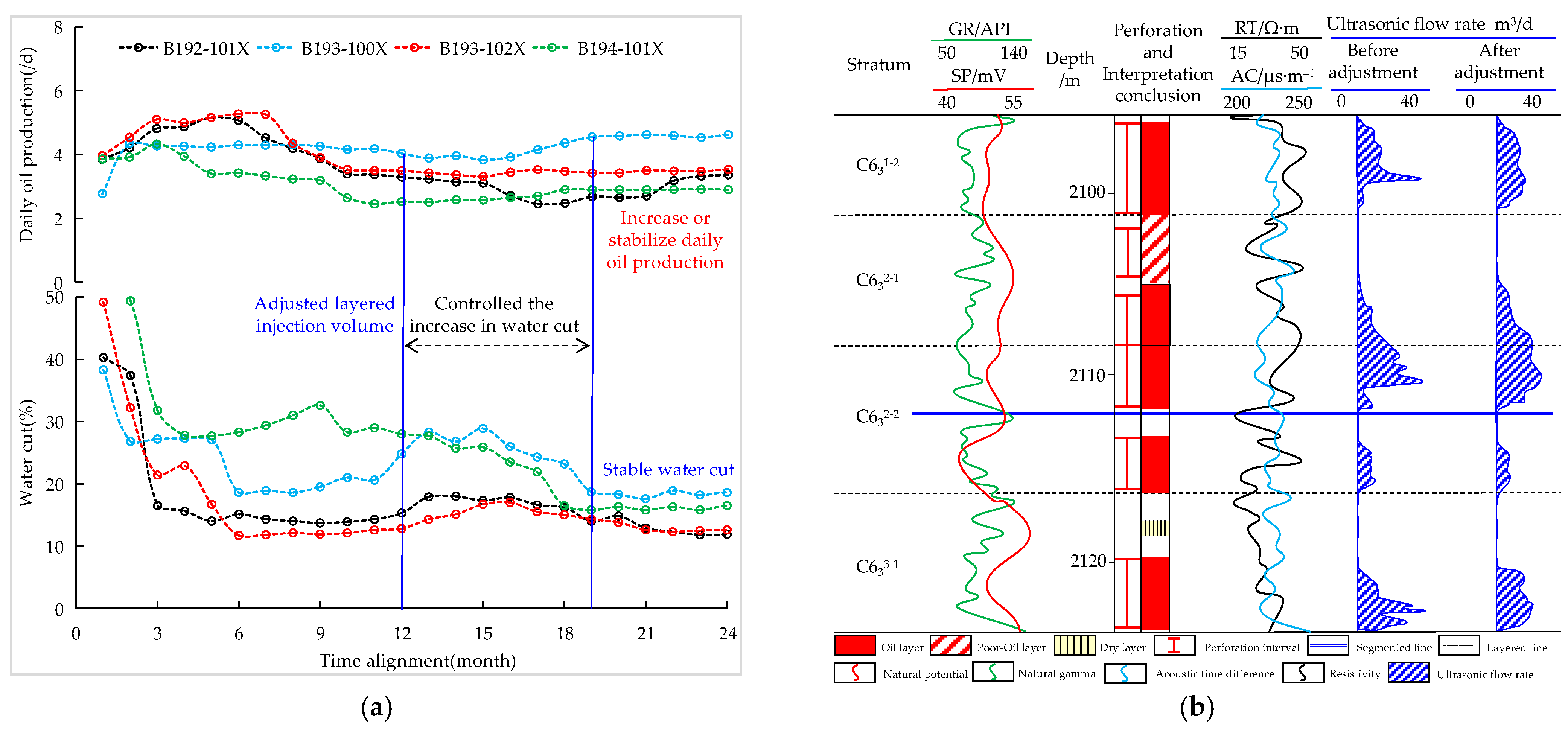
6. Production Dynamic Verification of the Layered Water Injection Adjustment Results
7. Conclusions
- (1)
- Four types of vertical stacking patterns and five types of lateral contact relationships of single sand body were identified using sand body configuration. The deposition rate and sediment recharge rate of the turbidite sedimentary system are fast, and the vertical multiperiod channel cutting and stacking type and lateral docking contact of the single sand body are the most developed. Through the combination of three methods of sand body configuration, seepage unit, and single sand body boundary identification, the accuracy of single sand body identification in the target area was 12.6% higher than that of sand body configuration identification.
- (2)
- The connectivity coefficient characterizes the connectivity ratio of sand bodies, the transition coefficient characterizes the connectivity strength of sand bodies, and the connectivity degree coefficient characterizes the real connectivity of sand bodies. The connectivity degree coefficient can be used as a standard for the quantitative evaluation of single sand body connectivity to determine the connectivity of single sand bodies.
- (3)
- In order to calculate the reasonable layered injection allocation of water injection reservoirs in highly deviated wells, it is suggested that three to five typical wells under different fracturing scales should be selected for microseismic monitoring, and the correlation between the fracture parameters and the ground fluid volume should be regressed to provide the basis for the lack of microseismic monitoring wells. According to the calculation results of the correlation formula, the fracture network is described, and the real displacement distance of oil and water wells in each layer of highly deviated wells is obtained.
- (4)
- The new methodology for determination of layered injection allocation in highly deviated wells drilled in low-permeability reservoirs clarifies the connectivity relationship between single sand bodies, describes the method for obtaining the real displacement distance of different layers in highly deviated wells, and determines the reasonable stratified injection allocation between layers. The method’s implementation resulted in a 3.6% reduction in the water cut by a year, and a significant increase in the daily oil production of individual wells by 0.5 t/d in the target area. The impact of the injection allocation adjustment was notably significant. This method is scientific and reasonable, simple and practical, convenient and fast, and has a good application value for the same type of highly deviated wells’ water injection development reservoirs.
Author Contributions
Funding
Data Availability Statement
Acknowledgments
Conflicts of Interest
References
- Qi, Z. Principles and Design of Oil Production Engineering; China University of Petroleum Press: Beijing, China, 2000. [Google Scholar]
- Hongwen, Y. A discussion using the techniques of production profile determination by the injection profiles of corresponding injection. Pet. Explor. Dev. 1990, 2, 47–55. [Google Scholar]
- Jianchuan, Y. Study on the Method of Calcuation and Optimization of Separated Layer Water Flooding Amount; Yangtze University: Jingzhou, China, 2015. [Google Scholar]
- Dongyi, Z. The Study of Single WELL injection Allocation Method in Cha Heji Oilfield; Southwest Petroleum University: Chengdu, China, 2006. [Google Scholar]
- Cao, L.; Xiu, J.; Cheng, H.; Wang, H.; Xie, S.; Zhao, H.; Sheng, G. A New Methodology for the Multilayer Tight Oil Reservoir Water Injection Efficiency Evaluation and Real-Time Optimization. Geofluids 2020, 2020, 8854545. [Google Scholar] [CrossRef]
- Xiaofei, J.; Qizheng, L.; Jing, Y.; Yunpeng, L.; Chunming, Z.; Yanchun, S. A method to allocate injection volume for separate layers in a water-injection well based on the remaining oil distribution. China Offshore Oil Gas 2012, 24, 38–40. [Google Scholar]
- Chuanzhi, C.; Hua, J.; Jiehong, D.; Yong, Y.; Jian, W. Reasonable injection rate allocation method of separate-layer water injection wells based on interlayer equilibrium displacement. Pet. Geol. Recovery Effic. 2012, 19, 94–96. [Google Scholar] [CrossRef]
- Zhaobo, S.; Yunpeng, L.; Xiaofei, J.; Yanlai, L.; Guohao, Z. A method to determine the layered injection allocation rates for water injection wells in high water cut oilfield based on displacement quantitative characterization. Pet. Drill. Tech. 2018, 46, 87–91. [Google Scholar] [CrossRef]
- Kuiqian, M.; Cunliang, C.; Yingxian, L. Separate-layer water injection allocation based on inter-layer balanced waterflooding. Spec. Oil Gas Reserv. 2019, 26, 109–112. [Google Scholar] [CrossRef]
- Qinglong, D.; Lihong, Z. A new approach to study layered producing performance of oil and water wells. Pet. Explor. Dev. 2004, 31, 96–98. [Google Scholar]
- Ling, L.; Bingguang, H.; Xingping, T.; Jianli, J.; Yidong, Z. Injection allocation rate determination of well groups using multiple regression method. Xinjiang Pet. Geol. 2006, 27, 357–358. [Google Scholar]
- Xinhua, W.; Jianlin, H.; Ke, A.; Yong, L. Application of BP neural network in well group injection allocation. Drill. Prod. Technol. 2006, 112–113. [Google Scholar]
- Zhou, Y.; Lei, S.; Du, X.; Ju, S.; Li, W. Injection-production optimization of carbonate reservoir based on an inter-well connectivity model. Energy Explor. Exploit. 2021, 39, 1666–1684. [Google Scholar] [CrossRef]
- Mamghaderi, A.; Bastami, A.; Pourafshary, P. Optimization of Waterflooding Performance in a Layered Reservoir Using a Combination of Capacitance-Resistive Model and Genetic Algorithm Method. J. Energy Resour. Technol. 2013, 135, 013102. [Google Scholar] [CrossRef]
- Zhang, L.; Xu, C.; Zhang, K.; Yao, C.; Yang, Y.; Yao, J. Production optimization for alternated separate-layer water injection in complex fault reservoirs. J. Pet. Sci. Eng. 2020, 193, 107409. [Google Scholar] [CrossRef]
- Yan, L.; Guangming, L.; Lili, S. Highly-deviated well in exploration and development of Zhangdian oilfield. Spec. Oil Gas Reserv. 2003, 37–39. [Google Scholar]
- Yu, Z.; Haiquan, Z.; Yongchen, L.; Chunqiu, G.; Haidong, S. Optimization of development of highly deviated well in gas reservoir with bottom water. Lithol. Reserv. 2015, 27, 114–118. [Google Scholar]
- Smith, R.W.; Colmenares, R.; Rosas, E.; Echeverria, I. Optimized reservoir development with high-angle wells, El Furrial field, Venezuela. SPE Reserv. Eval. Eng. 2001, 4, 26–35. [Google Scholar] [CrossRef]
- Fair, P.S.; Kikani, J.; White, C.D. Modeling high-angle wells in laminated pay reservoirs. SPE Reserv. Eval. Eng. 1999, 2, 46–52. [Google Scholar] [CrossRef]
- Abbas, A.K.; Rushdi, S.; Alsaba, M.; Al Dushaishi, M.F. Drilling Rate of Penetration Prediction of High-Angled Wells Using Artificial Neural Networks. J. Energy Resour. Technol. 2019, 141, 112904. [Google Scholar] [CrossRef]
- Ijasan, O.; Torres-Verdín, C.; Preeg, W.E.; Rasmus, J.; Stockhausen, E. Field examples of the joint petrophysical inversion of resistivity and nuclear measurements acquired in high-angle and horizontal wells. Geophysics 2014, 79, D145–D159. [Google Scholar] [CrossRef]
- Hu, X.; Fan, Y. Huber inversion for logging-while-drilling resistivity measurements in high-angle and horizontal wells. Geophysics 2018, 83, D113–D125. [Google Scholar] [CrossRef]
- Puzyrev, V.; Torres-Verdín, C.; Calo, V. Interpretation of deep directional resistivity measurements acquired in high-angle and horizontal wells using 3-D inversion. Geophys. J. Int. 2018, 213, 1135–1145. [Google Scholar] [CrossRef]
- Wang, L.; Wu, Z.-G.; Fan, Y.-R.; Huo, L.-Z. Fast anisotropic resistivities inversion of logging-while-drilling resistivity measurements in high-angle and horizontal wells. Appl. Geophys. 2021, 17, 390–400. [Google Scholar] [CrossRef]
- Duan, M.; Miska, S.; Yu, M.; Takach, N.; Ahmed, R.; Zettner, C. Critical Conditions for Effective Sand-Sized Solids Transport in Horizontal and High-Angle Wells. SPE Drill. Complet. 2009, 24, 229–238. [Google Scholar] [CrossRef]
- Wang, Y.; Zhou, C.; Yi, X.; Li, L.; Chen, W.; Han, X. Technology and Application of Segmented Temporary Plugging Acid Fracturing in Highly Deviated Wells in Ultradeep Carbonate Reservoirs in Southwest China. ACS Omega 2020, 5, 25009–25015. [Google Scholar] [CrossRef] [PubMed]
- Meng, F.; He, D.; Yan, H.; Zhao, H.; Zhang, H.; Li, C. Production performance analysis for slanted well in multilayer commingled carbonate gas reservoir. J. Pet. Sci. Eng. 2021, 204, 108769. [Google Scholar] [CrossRef]
- Waburoko, J.; Xie, C.; Ling, K. Effect of Well Orientation on Oil Recovery from Waterflooding in Shallow Green Reservoirs: A Case Study from Central Africa. Energies 2021, 14, 1223. [Google Scholar] [CrossRef]
- Wang, H.; Xue, S.; Gao, C.; Tong, X. Inflow performance for highly deviated wells in anisotropic reservoirs. Pet. Explor. Dev. 2012, 39, 239–244. [Google Scholar] [CrossRef]
- Wang, K.; Wang, L.; Adenutsi, C.D.; Li, Z.; Yang, S.; Zhang, L.; Wang, L. Analysis of Gas Flow Behavior for Highly Deviated Wells in Naturally Fractured-Vuggy Carbonate Gas Reservoirs. Math. Probl. Eng. 2019, 2019, 6919176. [Google Scholar] [CrossRef]
- Zhang, Q.; Zhang, L.; Liu, Q.; Jiang, Y. Pressure Performance of Highly Deviated Well in Low Permeability Carbonate Gas Reservoir Using a Composite Model. Energies 2020, 13, 5952. [Google Scholar] [CrossRef]
- Wang, L.; Lv, D.; Hower, J.C.; Zhang, Z.; Raji, M.; Tang, J.; Liu, Y.; Gao, J. Geochemical characteristics and paleoclimate implication of Middle Jurassic coal in the Ordos Basin, China. Ore Geol. Rev. 2022, 144, 104848. [Google Scholar] [CrossRef]
- Cui, J.; Li, S.; Mao, Z. Oil-bearing heterogeneity and threshold of tight sandstone reservoirs: A case study on Triassic Chang7 member, Ordos Basin. Mar. Pet. Geol. 2019, 104, 180–189. [Google Scholar] [CrossRef]
- Ding, F.; Shi, C.Q.; Zhang, P.H. Characteristics of the Braided River Deposits in the Tenth Member of Jurassic Yan’an Formation From Jiyuan Area in the Western Ordos Basin, China. Pet. Sci. Technol. 2013, 31, 2422–2430. [Google Scholar] [CrossRef]
- Tian, Y.; Yingchang, C.; Jingchun, T.; Xiaobing, N.; Shixiang, L.; Xinping, Z.; Jiehua, J.; Yian, Z. Deposition of deep-water gravity-flow hybrid event beds in lacustrine basins and their sedimentological significance. Acta Geol. Sin. 2021, 95, 3842–3857. [Google Scholar] [CrossRef]
- Xinping, Z.; Qing, H.; Jiangyan, L.; Shixiang, L.; Tian, Y. Features and origin of deep-water debris flow deposits in the Triassic Chang 7 Member, Ordos Basin. Oil Gas Geol. 2021, 42, 1063–1077. [Google Scholar] [CrossRef]
- Fudol, Y.A.; Zhao, Y.; Liu, H.; Zhou, S.; Li, Y.; Li, X. Origin and reservoir properties of deep-water gravity flow sediments in the Upper Triassic Ch6–Ch7 members of the Yanchang Formation in the Jinghe Oilfield, the Southern Ordos Basin, China. Energy Explor. Exploit. 2019, 37, 1227–1252. [Google Scholar] [CrossRef]
- Larue, D.K.; Hovadik, J. Connectivity of channelized reservoirs: A modelling approach. Pet. Geosci. 2006, 12, 291–308. [Google Scholar] [CrossRef]
- Lv, A.; Li, X.; Yu, M.; Li, G.; Wang, S.; Peng, R.; Zheng, Y. The method of the spatial locating of macroscopic throats based-on the inversion of dynamic interwell connectivity. Open Phys. 2017, 15, 313–322. [Google Scholar] [CrossRef]
- Gong, M.; Zhang, J.; Yan, Z.; Wang, J. Prediction of interwell connectivity and interference degree between production wells in a tight gas reservoir. J. Pet. Explor. Prod. Technol. 2021, 11, 3301–3310. [Google Scholar] [CrossRef]
- Yin, X.; Huang, W.; Lu, S.; Wang, P.; Wang, W.; Xia, L.; Yao, T. The connectivity of reservoir sand bodies in the Liaoxi sag, Bohai Bay basin: Insights from three-dimensional stratigraphic forward modeling. Mar. Pet. Geol. 2016, 77, 1081–1094. [Google Scholar] [CrossRef]
- Donselaar, M.E.; Overeem, I. Connectivity of fluvial point-bar deposits: An example from the Miocene Huesca fluvial fan, Ebro Basin, Spain. AAPG Bull. 2008, 92, 1109–1129. [Google Scholar] [CrossRef]
- Zhang, L.; Wang, H.; Li, Y.; Pan, M. Quantitative characterization of sandstone amalgamation and its impact on reservoir connectivity. Pet. Explor. Dev. 2017, 44, 226–233. [Google Scholar] [CrossRef]
- Yu, Z.; Yang, J.; Song, X.; Qiao, J. Fine Depiction of the Single Sand Body and Connectivity Unit of a Deltaic Front Underwater Distributary Channel: Taking the Third Member of the Dongying Formation in the Cha71 Fault Block of the Chaheji Oilfield as an Example. Geofluids 2021, 2021, 1401051. [Google Scholar] [CrossRef]
- Guangyi, H.; Tingen, F.; Fei, C.; Yongquan, J.; Laiming, S.; Xu, L.; Dakun, X. Theory of composite sand body architecture and its application to oilfield development. Oil Gas Geol. 2018, 39, 1–10. [Google Scholar] [CrossRef]
- Liu, R.; Sun, Y.; Wang, X.; Yan, B.; Yu, L.; Li, Z. Production Capacity Variations of Horizontal Wells in Tight Reservoirs Controlled by the Structural Characteristics of Composite Sand Bodies: Fuyu Formation in the Qian’an Area of the Songliao Basin as an Example. Processes 2023, 11, 1824. [Google Scholar] [CrossRef]
- Shi, T.; He, S.; Yuan, K.; Liu, M.; Wang, M.; Tu, X.; Chang, L. Analysis of Oil-Water Distribution Law and Main Controlling Factors of Meandering River Facies Reservoir Based on the Single Sand Body: A Case Study from the Yan 932 Layer of Y Oil Area in Dingbian, Ordos Basin. Geofluids 2023, 2023, 4273208. [Google Scholar] [CrossRef]
- Hearn, C.L.; Ebanks, W.J., Jr.; Tye, R.S.; Ranganathan, V. Geological factors influencing reservoir performance of the Hartzog Draw field, Wyoming. J. Pet. Technol. 1984, 36, 1335–1344. [Google Scholar] [CrossRef]
- Huanqing, C.; Yongle, H.; Lin, Y.; Min, T. Advances in the study of reservoir flow unit. Acta Geosci. Sin. 2010, 31, 875–884. [Google Scholar]
- Yang, Z.; Wang, S.; Chen, J.; Jing, S. Architecture, genesis, and the sedimentary evolution model of a single sand body in tight sandstone reservoirs: A case from the Permian Shan-1–He 8 members in the northwest Ordos Basin, China. Front. Earth Sci. 2023, 10, 1003818. [Google Scholar] [CrossRef]
- Ebanks, W.J., Jr. Flow unit concept-integrated approach to reservoir description for engineering projects. Am. Assoc. Pet. Geol. Bull. 1987, 71, 551–552. [Google Scholar]
- Shedid, S.A. A new technique for identification of flow units of shaly sandstone reservoirs. J. Pet. Explor. Prod. Technol. 2017, 8, 495–504. [Google Scholar] [CrossRef]
- Jie, A.; Meirong, T.; Zongxiong, C.; Wenxiong, W.; Wenbin, C.; Shunlin, W. Transformation of development model of horizontal wells in ultra-low permeability and low-pressure reservoirs. Lithol. Reserv. 2019, 35, 134–140. [Google Scholar] [CrossRef]
- Hanqiao, J.; Jun, Y.; Ruizhong, J. Principles and Methods of Reservoir Engineering; China University of Petroleum Press: Beijing, China, 2006. [Google Scholar]


| Parametric Classification | Factor Classification | Method Classification | Method Characteristics | Limitations |
|---|---|---|---|---|
| Single parameter | Geological factors | Effective thickness method [3] | The layered injection allocation is determined with the ratio of the oil-producing section to the total oil-producing section. | This method considers incomplete parameters. |
| Connected thickness method [4] | The layered injection allocation is determined with the ratio of the connected thickness of the sand body to the thickness of the oil well. | |||
| Development factors | Injection–production ratio method [3] | The layered injection allocation is ascertained by dividing the injection production ratio of each individual layer by the total injection production ratio. | The injection–production ratio of each layer is difficult to obtain. | |
| Liquid production intensity method [4] | The layered injection allocation is quantitatively analyzed through the multiplication of three factors: the perforation thickness, the connectivity coefficient, and the intensity of water injection in each layer. | The connectivity coefficient and water injection intensity data of each layer are difficult to obtain. | ||
| Multiparameter | Geological factors | Stratigraphic coefficient method [3] | Using the weighted formation coefficient, the water injection splitting coefficient of each layer is obtained. | This method considers incomplete parameters. |
| Sand body connectivity evaluation Stratigraphic coefficient method [5] | The sand body connectivity is divided into three categories by sedimentary facies, and the water injection is divided by combining the physical parameters. | The reason for sand body connectivity is not sufficient. | ||
| Remaining oil distribution method [6] | The layered injection allocation is obtained using the quantitative relationship between the recovery degree and the cumulative injection pore volume multiples. | The water absorption data acquisition is difficult. | ||
| Revised coefficient method [4] | Considering the injection–production balance, water cut rise rate, pump efficiency, and other factors, the empirical formula is obtained. | 1. This method considers many parameters and it is difficult to obtain some data. 2. There are many artificial coefficients, which easily cause errors. | ||
| Comprehensive factors | Splitting coefficient method [2] | According to geological conditions, oil displacement conditions, and mining conditions of the reservoir, the water injection volume is allocated according to the weight of the relevant parameters. | ||
| Balanced displacement method | Considering the physical properties and utilization status of each layer, the layered injection allocation relationship is established [7]. | 1. It is difficult to obtain layered recovery degree data. 2. The connectivity of sand bodies in each layer is not considered. | ||
| The layered injection allocation is obtained using the quantitative relationship between the recovery degree and the injection pore volume multiples [8]. | 1. This method requires a lot of experimental support, which cannot be replicated. 2. The connectivity of sand bodies in each layer is not considered. | |||
| The layered injection allocation is obtained using the idea of displacement flux equalization [9]. | This method does not consider the connectivity of sand bodies in each layer. | |||
| Seepage resistance coefficient method [10] | The vertical splitting coefficient of water injection well is determined using seepage resistance coefficient. | |||
| Mathematical model | Development factors | Multiple regression method [11] | A multiple sequence regression model is formulated, drawing from the dynamic production data of both the central water injection well and the surrounding production wells within the well group. | These methods are aimed at the optimization of well group injection allocation and cannot realize the optimization of layered injection allocation. |
| Neural network method [12] | The relationship model between liquid production and water injection is established using neural network technology. | |||
| Conductivity method [13] | The connectivity of the unit is characterized by its electrical conductivity and connected volume. | |||
| Capacitance–resistance method [14] | The formula for estimating water flooding in layered reservoirs is derived from the capacitance–resistance model equation. | This method considers many parameters, and it is difficult to obtain oil production and water injection of each layer. | ||
| Economic factors | Net present value method [15] | The water injection cycle, injection volume, and production should be adjusted based on the maximum net present value of production. | This method from the economic evaluation does not consider formation and development factors. |
| Evaluation Type | Evaluation Method | Method Characteristics | Limitations |
|---|---|---|---|
| Inter-well connectivity | Dynamic monitoring method | The connectivity between oil and water wells is judged using dynamic monitoring data [39,40]. | This method cannot judge the inter-well connectivity without dynamic monitoring data or seismic data interpretation. |
| inter-sand body connectivity | Seismic method | Based on seismic data, the connectivity of the sand body is analyzed [41]. | |
| Sand–ground ratio method | The connectivity of sand body is judged using the sedimentary structure model of sand body described by outcrop [42]. | 1. The accuracy of this method is low; 2. The method cannot effectively identify the sedimentary interface; 3. The method cannot clarify the connectivity between different sand bodies. | |
| Sandstone amalgamation method | Through the identification of sand mud facies, the degree of sandstone amalgamation is described. The higher the amalgamation rate, the better the connectivity [43]. | ||
| Sand body configuration method | By analyzing the contact relationship of sand bodies, the connectivity of sand bodies is determined [44]. | This method cannot clarify the connectivity and degree of connectivity between different sand bodies. |
| Contact Type | Contact Relationship | Flow Unit Type | Elevation Difference (Yes/No) | Contact Mode | Connectivity | Transition Coefficient |
|---|---|---|---|---|---|---|
| Lateral | Connection (same sand body) | Same kind | No | 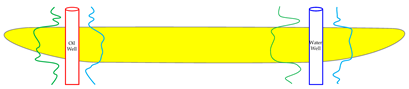 | Perfect | 1.0 |
| Lateral cut type or substitution type (different sand body) | Same kind | No | 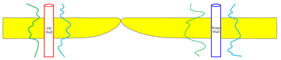 | Good | 0.9 | |
| Yes | 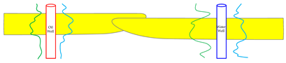 | Medium-good | 0.8 | |||
| Class I and II or Class II and III | Yes | 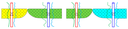 | Medium | 0.6 | ||
| Lateral | Lateral cut type or substitution type (different sand body) | Class I and II or Class II and III | Yes | 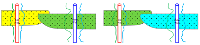 | Medium-poor | 0.4 |
| Class I and III | No |  | Medium-poor | 0.4 | ||
| Yes | 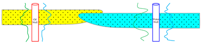 | Poor | 0.2 | |||
| Vertical | Cut and stack type | Same Kind |  | Good | 1.0 | |
| Class I and II or Class II and III |  | Medium | 0.6 | |||
| Class I and III |  | Poor | 0.4 | |||
   | ||||||
| Section | Fracture Length (m) | Fracture Width (m) | Fracture Height (m) | Fracture Strike (Northeast) | ||
|---|---|---|---|---|---|---|
| West Flank | East Flank | Overall Length | ||||
| The first section | 128 | 46 | 174 | 41 | 76 | 57° |
| The second section | 159 | 131 | 290 | 62 | 49 | 61° |
| The third section | 220 | 126 | 346 | 58 | 59 | 63° |
| The fourth section | 267 | 134 | 401 | 60 | 60 | 66° |
| The fifth section | 128 | 96 | 224 | 44 | 43 | 58° |
| Well Name | Fracturing Section | Real Displacement Distance (m) | Sand Body Connectivity (Yes/No) | Connectivity Degree Coefficient | Permeability (mD) | Effective Thickness (m) | Displacement Coefficient | Water Injection Section | Displacement Coefficient of Water Injection Section | Layered Injection Ratio | Layered Injection Calculation (m3) |
|---|---|---|---|---|---|---|---|---|---|---|---|
| B192-101x | 1 | 85 | Yes | 0.9 | 0.23 | 1.56 | 27.4 | Upper section | 199.5 | 0.72 | 14.5 |
| 2 | 150 | Yes | 0.8 | 0.23 | 4.77 | 131.7 | |||||
| 3 | 110 | Yes | 0.8 | 0.14 | 3.28 | 40.4 | |||||
| 4 | 150 | No | 0.16 | 0.91 | 0 | Lower section | 76.6 | 0.28 | 5.5 | ||
| 5 | 110 | Yes | 1.0 | 0.2 | 3.48 | 76.6 | |||||
| 6 | 140 | No | 0.16 | 2.98 | 0 | ||||||
| B194-101x | 1 | 120 | Yes | 0.8 | 0.25 | 2.71 | 65.0 | Upper section | 261.8 | 0.62 | 12.4 |
| 2 | 140 | Yes | 1.0 | 0.18 | 5.66 | 142.6 | |||||
| 3 | 160 | Yes | 0.9 | 0.33 | 1.14 | 54.2 | |||||
| 4 | 160 | Yes | 0.8 | 0.3 | 4.17 | 160.1 | Lower section | 160.1 | 0.38 | 7.6 | |
| 5 | 190 | No | 0.24 | 3.29 | 0 | ||||||
| B193-100x | 1 | 160 | Yes | 1.0 | 0.19 | 2.15 | 65.4 | Upper section | 228.2 | 0.72 | 14.4 |
| 2 | 160 | Yes | 1.0 | 0.22 | 3.71 | 130.6 | |||||
| 3 | 100 | Yes | 0.8 | 0.21 | 1.92 | 32.3 | |||||
| 4 | 110 | No | 0.24 | 1.79 | 0 | Lower section | 87.7 | 0.28 | 5.6 | ||
| 5 & 6 | 90 | Yes | 1.0 | 0.22 | 4.43 | 87.7 | |||||
| B193-102x | 1 | 150 | Yes | 0.8 | 0.18 | 2.12 | 45.8 | Upper section | 144.4 | 0.63 | 12.7 |
| 2 | 150 | Yes | 1.0 | 0.18 | 1.24 | 33.5 | |||||
| 3 | 165 | Yes | 0.8 | 0.21 | 2.35 | 65.1 | |||||
| 4 | 180 | No | 0.24 | 1.68 | 0 | Lower section | 83.1 | 0.37 | 7.3 | ||
| 5 | 180 | Yes | 0.9 | 0.18 | 2.85 | 83.1 |
Disclaimer/Publisher’s Note: The statements, opinions and data contained in all publications are solely those of the individual author(s) and contributor(s) and not of MDPI and/or the editor(s). MDPI and/or the editor(s) disclaim responsibility for any injury to people or property resulting from any ideas, methods, instructions or products referred to in the content. |
© 2023 by the authors. Licensee MDPI, Basel, Switzerland. This article is an open access article distributed under the terms and conditions of the Creative Commons Attribution (CC BY) license (https://creativecommons.org/licenses/by/4.0/).
Share and Cite
Li, M.; Qu, Z.; Ji, S.; Bai, L.; Yang, S. A New Methodology for Determination of Layered Injection Allocation in Highly Deviated Wells Drilled in Low-Permeability Reservoirs. Energies 2023, 16, 7764. https://doi.org/10.3390/en16237764
Li M, Qu Z, Ji S, Bai L, Yang S. A New Methodology for Determination of Layered Injection Allocation in Highly Deviated Wells Drilled in Low-Permeability Reservoirs. Energies. 2023; 16(23):7764. https://doi.org/10.3390/en16237764
Chicago/Turabian StyleLi, Mao, Zhan Qu, Songfeng Ji, Lei Bai, and Shasha Yang. 2023. "A New Methodology for Determination of Layered Injection Allocation in Highly Deviated Wells Drilled in Low-Permeability Reservoirs" Energies 16, no. 23: 7764. https://doi.org/10.3390/en16237764