Article

Exploring Time Series Models for Wind Speed Forecasting: A Comparative Analysis

1
School of Statistics, Capital University of Economics and Business, Beijing 100070, China
2
School of Finance, Capital University of Economics and Business, Beijing 100070, China
*
Author to whom correspondence should be addressed.
Energies 2023, 16(23), 7785; https://doi.org/10.3390/en16237785
Submission received: 2 November 2023 / Revised: 14 November 2023 / Accepted: 17 November 2023 / Published: 27 November 2023
(This article belongs to the Section A3: Wind, Wave and Tidal Energy)

Abstract

:
The sustainability and efficiency of the wind energy industry rely significantly on the accuracy and reliability of wind speed forecasting, a crucial concern for optimal planning and operation of wind power generation. In this study, we comprehensively evaluate the performance of eight wind speed prediction models, spanning statistical, traditional machine learning, and deep learning methods, to provide insights into the field of wind energy forecasting. These models include statistical models such as ARIMA (AutoRegressive Integrated Moving Average) and GM (Grey Model), traditional machine learning models like LR (Linear Regression), RF (random forest), and SVR (Support Vector Regression), as well as deep learning models comprising ANN (Artificial Neural Network), LSTM (Long Short-Term Memory), and CNN (Convolutional Neural Network). Utilizing five common model evaluation metrics, we derive valuable conclusions regarding their effectiveness. Our findings highlight the exceptional performance of deep learning models, particularly the Convolutional Neural Network (CNN) model, in wind speed prediction. The CNN model stands out for its remarkable accuracy and stability, achieving the lowest mean squared error (MSE), root mean squared error (RMSE), mean absolute error (MAE), mean absolute percentage error (MAPE), and the higher coefficient of determination ( R 2 ). This underscores the CNN model’s outstanding capability to capture complex wind speed patterns, thereby enhancing the sustainability and reliability of the renewable energy industry. Furthermore, we emphasized the impact of model parameter tuning and external factors, highlighting their potential to further improve wind speed prediction accuracy. These findings hold significant implications for the future development of the wind energy industry.

1. Introduction

In today’s society, the urgent need to address global climate change and the demand for sustainable energy sources have brought clean, renewable energy forms to the forefront [1,2]. As we strive to reduce our reliance on traditional fossil fuels, cut down greenhouse gas emissions, and work towards achieving carbon neutrality goals, wind energy is gaining widespread attention and acclaim. Wind energy, as a clean, economical, and renewable energy source, holds immense potential to provide us with clean electricity while alleviating our carbon footprint and meeting the ever-growing power requirements [3].
However, despite the significant advantages of wind energy, it comes with its own set of challenges, one of which is its inherent uncertainty and variability. Wind energy generation is influenced by fluctuations in wind speeds, posing challenges for its effective integration into the power grid. Consequently, in the wind energy sector, wind speed forecasting has become a critical component. Wind speed directly impacts the output of wind turbines, which are at the heart of wind energy conversion systems. Therefore, accurate wind speed prediction is crucial for the safety of the electrical grid and the efficient operation of wind power systems. Precise wind speed forecasting contributes not only to ensuring the reliability of wind energy systems but also to enhancing energy supply stability, reducing operational costs, and aiding in the pursuit of carbon neutrality goals. Additionally, possessing reliable uncertainty information in forecasts can mitigate risks in the planning of wind energy systems, instilling confidence and feasibility for investors and operators.
To meet the demands of wind speed prediction, researchers and engineers have been exploring various wind speed forecasting methods. These methods can be broadly categorized into three major classes: statistical learning methods, traditional machine learning methods, and deep learning methods. Although various methods exhibit potential in the field of wind speed prediction, there is currently a lack of comprehensive comparison among them. Understanding the performance and advantages of different methods is crucial for determining which one to choose in specific circumstances. Therefore, this study aims to conduct a comprehensive comparative analysis of eight wind speed prediction models: AutoRegressive Integrated Moving Average (ARIMA) and the Grey Model (GM), Linear Regression (LR), random forest (RF), Support Vector Regression (SVR), Long Short-Term Memory (LSTM), Artificial Neural Network (ANN), and Convolutional Neural Network (CNN). The objective of this research is to determine which model performs best in various scenarios, providing more accurate wind speed forecasting tools for the wind energy industry and contributing to the achievement of carbon neutrality goals. Through in-depth performance comparisons, our study will offer valuable insights for decision makers, engineers, and investors, optimizing the operation and planning of wind power systems, and advancing a cleaner and more sustainable future, thereby contributing to the realization of carbon neutrality goals.
In recent years, the field of wind speed prediction has witnessed significant advancements, with researchers proposing various models to address this challenge. These models can be broadly categorized into three types: statistical models, traditional machine learning models, and deep learning models. Statistical models encompass traditional time series methods such as ARIMA and models based on physical principles. Traditional machine learning models include decision trees, random forests, support vector machines, and others, showcasing a strong performance in data-driven wind speed prediction. Simultaneously, deep learning models like Recurrent Neural Networks (RNNs) and CNNs have garnered considerable attention due to their proficiency in handling complex nonlinear relationships. The following literature review will delve into the applications and performances of these three major model categories, aiming to provide a comprehensive understanding of their utility.
In the field of wind speed prediction, the application of statistical models exhibits varied and significant potential. Ref. [4] introduced a short-term wind speed prediction method based on gray system theory, successfully applied in the Dafeng region of Jiangsu province, China, and providing accurate data for short-term wind energy assessment. Ref. [5] proposed an innovative wind speed prediction method that utilizes Variational Mode Decomposition (VMD) to decompose wind speed into nonlinear, linear, and noise components. Models for each component were constructed, enhancing the stability of wind power systems. However, ref. [6] investigated nested ARIMA models, which effectively captured wind speed fluctuations but exhibited notable differences in extreme fluctuation distributions. Ref. [7] compared various time series models and found that BATS and ARIMA performed best on test data. Ref. [8] further improved the gray system model by introducing fractional-order gray system models and a neural network-based combination prediction model, significantly enhancing prediction accuracy. Finally, ref. [9] employed a Polynomial AutoRegressive (PAR) model for wind speed and power prediction, and the results demonstrated the superiority of the PAR model when predicting wind speed and power, with a forecast horizon exceeding 12 h. These studies provide a range of methods for wind speed prediction, although their performance and applicability are influenced by variations in data and geographical locations, collectively offering substantial support to the wind energy industry.
In the field of wind speed prediction, research on traditional machine learning models has made significant strides, providing robust tools to enhance prediction accuracy and reliability. Ref. [10] introduced a wind speed probability distribution estimation method based on the law of large numbers and integrated it with an SVR model, demonstrating its remarkable effectiveness through experimental results. Ref. [11] applied the ANN model to wind speed prediction at micro-level locations, serving as a decision support tool for early warning systems and underscoring the feasibility of ANNs in the prediction process. Ref. [12] introduced a weighted RF model optimized by wavelet decomposition and a specialized algorithm for ultra-short-term wind power prediction, exhibiting exceptional accuracy and stability in the presence of noise and unstable factors. Ref. [13] proposed a short-term wind power prediction model that employs two-stage feature selection and supervised RF optimization, showing superior accuracy, efficiency, and stability, particularly in scenarios with high noise data and wind power curtailment. Additionally, ref. [14] introduced a ν-SVR model tailored for complex noise in short-term wind speed forecasting, achieving significant performance improvements. Finally, ref. [15] employed kernel-based Support Vector Machine Regression models, comparing various kernel functions and highlighting the superior performance of the Pearson VII SVR model. Collectively, these studies underscore the pivotal role of traditional machine learning models in the field of wind speed prediction, providing diverse methods and pathways for various application scenarios, thereby enhancing prediction accuracy and positively impacting the wind energy industry and renewable energy management.
Deep learning models have achieved remarkable advancements in the field of wind speed prediction, offering powerful tools to enhance prediction accuracy and reliability. Ref. [16] utilized 13 years of wind speed data from the Qaisumah region and established an Artificial Neural Network model, demonstrating its outstanding performance with low mean square error (MSE) and mean absolute percentage error (MAPE) values. Ref. [17] introduced a multi-wind farm wind speed prediction strategy tailored to centralized control centers, leveraging the deep learning model Bi-LSTM and transfer learning to achieve high accuracy and broad applicability. Ref. [18] presented a hybrid model for wind speed interval prediction, using an autoencoder and bidirectional LSTM neural network, highlighting the feature extraction effectiveness of the autoencoder in time series forecasting. Ref. [19] focused on the prediction of wind speeds at multiple locations, introducing a two-layer attention-based LSTM model named 2Attn-LSTM, which encodes spatial features and decodes temporal features through variational mode decomposition, outperforming four baseline methods. Ref. [20] proposed an indirect approach to wind direction prediction by decomposing wind speed into crosswind and along-wind components, utilizing LSTM models and Empirical Mode Decomposition (EMD) to predict these components, thereby enabling wind direction prediction. The effectiveness of this approach was demonstrated using one month of wind monitoring data. Ref. [21] introduced a wind speed prediction model based on an LSTM neural network optimized using the Firework Algorithm (FWA) to enhance hyperparameter performance. Focusing on the real-time dynamics and dependencies in wind speed data, the optimized model demonstrated a reduction in prediction errors and improved accuracy compared with other deep neural architectures and regression models. Ref. [22] presented a hybrid PCA and LSTM prediction method, leveraging PCA for meteorological data preprocessing and optimizing LSTM with the DE algorithm for superior predictive performance, particularly in wind speed prediction. Ref. [23] developed a hybrid deep learning model for short-term wind speed forecasting, with a comparative analysis showing that the CNN-BLSTM consistently outperformed other models across various time series and heights. Ref. [24] introduced a custom-designed CNN-based deep learning model for solar wind prediction, effectively tracking solar wind back to its source at the Sun, derived from AIA images, and predicting solar wind speed. Ref. [25] presented a hybrid deep learning model for wind speed prediction, combining CNN and LSTM architectures, achieving a test RMSE of 1.84 m/s. The model’s track-wise processing approach outperformed other models, showcasing the potential of capturing spatiotemporal correlations among data along a trajectory for improved accuracy. Ref. [26] introduced an improved wind power prediction model using a combination of Convolutional Neural Networks and the Informer model to enhance prediction accuracy, based on real wind farm data from China. Ref. [27] employed deep learning and extreme ultraviolet images to predict solar wind properties, outperforming traditional models with a correlation of 0.55 ± 0.03. Model analysis revealed its ability to capture correlations between solar corona structures and wind speeds, offering potential data relationships for solar physics research. These studies collectively highlight the outstanding performance and extensive applicability of deep learning models in the domain of wind speed prediction, providing robust support for the wind energy industry and renewable energy management. Different models and approaches offer different advantages in various application scenarios, contributing to the continuous improvement of wind speed prediction accuracy.
In summary, the field of wind speed prediction has seen significant advancements, with the emergence of various promising models and methods, including statistical models, traditional machine learning models, and deep learning models. These studies have greatly improved the accuracy and reliability of wind speed prediction, providing essential impetus for the wind energy industry and renewable energy management. However, despite the distinct advantages exhibited by different types of models in specific contexts, there is currently a lack of comprehensive model comparison research that can assist researchers in selecting the most suitable models for their specific application needs. This is where the value of our study lies. We will conduct a comprehensive comparative analysis of statistical models, traditional machine learning models, and deep learning models to evaluate their performance. By addressing this research gap, our study will provide a comprehensive model comparison framework for other scholars, aiding them in making better-informed choices for wind speed prediction models that align with their research and practical applications. This will further drive advancements in the field of wind speed prediction and promote the sustainable growth of the renewable energy industry.
The main contributions of this paper are as follows: (1) A comprehensive performance comparison: This study plans to conduct an extensive comparative analysis, including eight different wind speed prediction models, spanning statistical models, traditional machine learning, and deep learning methods. This comprehensive performance comparison aims to provide in-depth insights into the performance of different models, helping decision makers determine which model is most suitable for short-term wind speed forecasting in various contexts. (2) Real-world validation and performance optimization: The research validates the performance of eight machine learning models in short-term wind speed prediction using real-world case study data. This practical validation not only underscores the feasibility of these models but also offers robust support and profound insights for optimizing the performance of actual wind energy systems.
The remainder of this article is arranged as follows: In Section 2, an initial presentation of the technical roadmap for the research framework will be provided, followed by a detailed description of eight distinct wind speed prediction models, encompassing statistical models, traditional machine learning, and deep learning models. Additionally, this section will outline the data sources and experimental design used for model training and evaluation. In Section 3, we will present the primary findings of the study, including a performance comparison of the various models, utilizing charts, data analysis, and performance metrics to showcase the models’ performance. Finally, in Section 4, the article will summarize the main findings, emphasize key insights from the model comparisons, provide an in-depth discussion of these results, and also consider the limitations of the study and directions for future work.

2. Methods and Data

2.1. Technology Roadmap

This study aims to comprehensively compare eight different types of time series forecasting models, including traditional statistical models (GM and ARIMA), traditional machine learning models (LR, RF, and SVR), and deep learning models (ANN, LSTM, and CNN). Figure 1 displays the technical roadmap, and the subsequent sections offer in-depth explanations of these three stages in the technical roadmap:
Stage one: Data preparation. In the first stage, we perform data preparation to lay the foundation for subsequent model comparisons and evaluations. Firstly, we carefully collect actual wind power data from two Chinese wind farms, with a time span of fifteen minutes. Then, we conduct necessary data engineering and cleaning to ensure data quality and consistency, including handling missing values and outlier data. Finally, we divide the entire dataset into two parts, with the first 80% designated as the training set and the remaining 20% as the test set.
Stage two: Modeling process. In the second stage, we delve into the modeling process, training and adjusting parameters for each model to adapt to the time series characteristics of wind speed data. We provide the dataset to different types of models, including statistical models (GM and ARIMA), traditional machine learning models (LR, RF, and SVR), and deep learning models (ANN, LSTM, and CNN). The key task in this stage is to ensure that each model can make the most of the data through parameter tuning and training to enhance its performance.
Stage three: Model evaluation and selection. In the third stage, we carry out model evaluation and selection to determine which model performs best in short-term wind power forecasting. We use five different model evaluation metrics, including mean squared error (MSE), root mean square error (RMSE), mean absolute error (MAE), mean absolute percentage error (MAPE), and R-squared (R-square), to comprehensively assess the performance of the eight models. This stage will assist us in selecting the most suitable model for short-term wind speed forecasting, ultimately providing a reliable forecasting tool for the wind power industry.

2.2. Model

2.2.1. GM Model

The Gray Model (GM) is a time series forecasting method used to handle relatively small amounts of data and information, particularly suitable for situations involving incomplete, unevenly distributed, or data-poor scenarios [28]. The core concept of the GM model is to divide data into “white” information and “black” information and use modeling and fitting techniques to estimate the “black” information, thus enhancing the accuracy of predictions. The main types of GM models include the GM(1,1) and GM(2,n) models, with GM(1,1) being the most commonly used one. The modeling process of the GM(1,1) model typically involves the following steps:
Step 1. Data preprocessing: First, the original data series X ( 0 ) , X ( 1 ) , X ( 2 ) , , X ( n ) is cumulatively processed to obtain the close-to-average value sequence Z ( 0 ) , ( 1 ) , ( 2 ) , , Z ( n ) . The accumulation operation is typically performed using the following formula:
Z ( k ) = i = 1 k X ( i ) , i = 1,2 , , n
Step 2. Establishing difference equations: Using the close-to-average value sequence Z ( k ) and the original data series X ( k ) , difference equations are established, typically represented as
X ( k ) + a · Z ( k ) = X ( 0 ) + b , k = 1,2 , , n
where a and b are model parameters that need to be estimated.
Step 3. Parameter estimation: To estimate parameters a and b, the least squares method is typically employed. By replacing k in the difference equation with k − 1, you can derive the following linear fitting equation:
X ( k ) = a · Z ( k ) + X ( 0 ) + b , k = 1,2 , , n
Data points (Z(k), X(k)) are considered as points in a coordinate system, and the least squares method is used to fit the straight line a · Z ( k ) + X(0) + b to estimate parameters a and b.
Step 4. Verification of fitting quality: Once parameters a and b are obtained, these parameters are used to verify the quality of the model’s fit. Typically, metrics are used to evaluate the fitting performance.
The Gray Model is suitable for handling small-sample data, characterized by simplicity and adaptability to nonlinear systems. Its strengths lie in strong adaptability, robustness to uncertainties, and simplified modeling, making it particularly well-suited for short-term forecasting and managing incomplete information scenarios. Therefore, in situations with limited resources or constrained data availability, the Gray Model serves as an effective mathematical modeling tool.

2.2.2. ARIMA Model

The AutoRegressive Integrated Moving Average (ARIMA) model is a classic time series forecasting method used to analyze and predict trends and seasonality in time series data. It consists of three main components: AutoRegressive (AR), Integrated (I), and Moving Average (MA) [29]. Below is an explanation of the ARIMA model’s principles.
AutoRegressive (AR): The AR component of the ARIMA model represents the relationship between the current observation and past observations at several previous time steps. In an AR(p) model, the current observation depends on the values of the previous p time steps. The formula is as follows:
X t = c + φ 1 X t 1 + φ 2 X t 2 + + φ p X t p + ε t
where X t represents the current observation, X t 1 , X t 2 , …, X t p represent the values of the time series at the previous p time steps, φ 1 , φ 2 , …, φ p are the auto-regressive coefficients, c is the intercept, and ε t represents the error term.
Integrated (I): The I component of the ARIMA model involves differencing the original data to make the time series stationary. The differencing order is usually denoted as d. The differencing operation transforms a nonstationary time series into a stationary one, and it is represented as
Y t = X t X t d
where Y t represents the differenced time series.
Moving Average (MA): The MA component of the ARIMA model represents the relationship between the current observation and past error terms at several previous time steps. In an MA(q) model, the current observation depends on the values of q past error terms. The formula is as follows:
X t = c + ε t + θ 1 ε t 1 + θ 2 ε t 2 + + θ q ε t q
where   ε t   represents the current error term, and ε t 1 , ε t 2 , …, ε t q represent the error terms at previous q time steps. θ 1 , θ 2 , …, θ q are the moving average coefficients, and c is the intercept.
The ARIMA (AutoRegressive Integrated Moving Average) model is a classic method capable of effectively handling seasonal variations in time series data. Its strengths lie in simplicity, interpretability of parameters, and applicability to short-term forecasting and economic time series analysis. It is particularly well-suited for scenarios with relatively stable demands and moderate variations.

2.2.3. LR Model

A linear regression model can be used for single-variable time series forecasting [30]. The basic principle is to establish a linear relationship between the current time’s observation and the observations from previous time steps. The following are the detailed principles:
Assuming we have a single-variable time series { y 1 , y 2 , …, y t }, where y t represents the observation at time t, the objective of the linear regression model is to establish a linear relationship between the current time’s observation y t and the observations from previous time steps. The basic form of the linear regression model is as follows:
y t = β 0 + β 1 · y t 1 + ε t
where y t is the observation at time t, which is the target value we want to predict. β 0 is the intercept of the model, representing the average value in the absence of other influences. β 1 is the autoregressive coefficient, representing the influence of the observation at the previous time step (t − 1) on the current time step. y t 1 is the observation at the previous time step (t − 1). ε t is the error term, representing the unaccounted random noise in the model. The goal is to estimate the parameters β 0 and β 1 , which can be accomplished through techniques like least squares or other regression methods. Once these parameters are estimated, the model can be used for forecasting.
The strength of the linear regression model lies in its simplicity, ease of use, and excellent interpretability, making it suitable for scenarios where data exhibits a clear linear relationship. However, its performance may be suboptimal when dealing with nonlinear relationships and outliers, and it requires strong assumptions about the data. Therefore, it is well-suited for addressing straightforward linear problems, especially in situations where the data are relatively simple and exhibit an evident linear relationship.

2.2.4. RF Model

When applying the RF model for regression tasks, the basic principles include data sampling, tree construction, and integration of prediction results [31]. The following is the basic principles of the RF model:
Step 1. Data sampling: Randomly select multiple subsets from the training data, which can be chosen with replacement (Bootstrap sampling). These subsets will be used to build different decision trees. Specifically, let D represent the original dataset, and D’ represent the subset after Bootstrap sampling. D’ contains n randomly selected samples, where n ≤ |D|.
Step 2. Tree construction: For each subset D’, construct a decision tree. The tree construction process typically uses a recursive approach by selecting the best splitting features and splitting points to fit the data. The tree construction process involves tree splitting, node rules, and calculation of output values in leaf nodes, typically using criteria based on mean squared error (MSE).
Step 3. Integration of prediction results: For regression problems, the final prediction result of the RF model is the average of the prediction results from each decision tree. The mathematical expression is
y ~ = 1 N i = 1 N f i ( x )
where y ~ is the final regression prediction of the random forest. N is the number of decision trees in the random forest. f i ( x ) is the prediction result of the i-th decision tree.
Random forest reduces overfitting risk, enhances model robustness, and typically yields accurate regression predictions by combining the prediction results of multiple decision trees. The structure of the RF model is shown in Figure 2. The RF model excels in high accuracy, sensitivity to nonlinear relationships, and feature importance assessment. However, it is considered a black-box model with substantial computational costs and potential risks of overfitting. It is well-suited for handling complex data patterns and conducting feature importance analysis, and it performs exceptionally in prediction tasks where high accuracy is paramount.

2.2.5. SVR Model

Support Vector Regression (SVR) is a machine learning method used for regression analysis. The core idea behind SVR is to find a regression function that minimizes the error between predicted values and actual values [32]. SVR is based on the Support Vector Machine (SVM) approach and is used to handle regression problems. The following is the detailed principles of the SVR model:
  • Data representation: Assume you have a training dataset containing input features X and corresponding target values y, where X is an n-dimensional feature vector. The goal of regression is to find a function f ( X ) that can predict y.
  • Maximizing the margin: The key idea of SVR is to find a regression function by maximizing the margin. It seeks to find the hyperplane with the largest margin, which maximizes the distance between the hyperplane and data points (support vectors).
  • Regression function: The regression function in SVR is generally represented as
y = f ( X ) = < w , X > + b
where y is the predicted target value. X is the input feature vector. w is the weight vector used to determine the direction of the hyperplane. b is the bias term.
4.
Margins and constraints: SVR seeks to find the best hyperplane while satisfying the following constraints:
| y < w , X > b | ϵ
where ϵ is a user-defined parameter that controls the size of the margin.
5.
Loss function: SVR uses a loss function, typically using MSE or mean absolute error (MAE), to quantify the error between predicted values and actual values. The goal of SVR is to minimize this loss function. The MSE loss function is
L < y , < w , X > + b > = 1 2 ( y < w , X > b ) 2
6.
Minimization problem: SVR solves the following convex optimization problem to find the best regression function:
min w , b 1 2 | | w | | 2 + C i = 1 n ( L ( y i , < w , X i > + b ) ϵ )
where | | w | | 2 is the norm of the weight vector w, C is the regularization parameter, and n is the number of data points.
7.
Kernel functions: SVR can use kernel functions, such as linear, polynomial, or radial basis function (RBF) kernels, to handle nonlinear regression problems. Kernel functions map input features to a higher-dimensional space, allowing linear regression models to capture nonlinear relationships.
SVR model excels in high-dimensional spaces, robustness to outliers, and flexibility in choosing different kernel functions. However, it comes with the drawback of high computational costs, sensitivity to parameter tuning, and limited interpretability. It is well-suited for regression in high-dimensional spaces, scenarios with outliers, and problems requiring the flexibility of different kernel functions.

2.2.6. ANN Model

Artificial neural networks (ANNs) are computational models inspired by the structure of the human brain. They consist of interconnected nodes or artificial neurons organized into layers, including input, hidden, and output layers [33]. ANN model has the ability to learn and generalize patterns from data, making it a powerful tool for time series forecasting. Using the ANN model for single-variable time series forecasting is a powerful and flexible approach. Time series data often exhibit complex, nonlinear patterns, and ANNs are well-suited to capture these intricate relationships. In this context, ANNs can be used to make predictions based on historical data, allowing us to anticipate future values of a single variable. The structure of the ANN model is shown in Figure 3. Below is a brief introduction to how ANNs are applied to single-variable time series forecasting:
1.
Neural network architecture:
Input layer: The input layer typically consists of neurons corresponding to lagged observations in the time series. If you choose to use the previous m observations as inputs, the input layer will have m neurons.
Hidden layers: Hidden layers are used to capture nonlinear relationships within the time series. You can have one or more hidden layers, each containing multiple neurons. The depth (number of layers) and width (number of neurons per layer) of the ANN are adjustable hyperparameters.
Output layer: The output layer usually contains a single neuron that is responsible for outputting the prediction of the time series.
2.
Functioning of neurons: Each neuron performs the following operations:
Weighted sum: The neuron multiplies input signals by their respective weights and sums them up. This computes the weighted sum of the input features, represented by the following formula:
z = i = 1 n ( w i · x i ) + b
where z is the weighted sum of the neuron. w i is the weight of the i-th input feature. x i is the value of the i-th input feature. b is the neuron’s bias term.
Activation function: The weighted sum z is typically passed through an activation function to produce the neuron’s output. Common activation functions include Sigmoid, Rectified Linear Unit (ReLU), tanh, and others.
a = f ( z )
where a is the neuron’s output. f ( z ) is the activation function.
1.
Training the neural network:
Loss function: This measures the error between predicted values and actual values. For regression tasks, MSE is commonly used as the loss function.
Backpropagation: Optimization algorithms like gradient descent are used to minimize the loss function by updating the weights and biases throughout the network through backpropagation of errors.
2.
Prediction:
Once training is complete, you can use the trained neural network to make predictions for a single-variable time series. Input the past observations as input to the network, and it will generate future prediction values.
The ANN model possesses robust capabilities in nonlinear modeling, making it suitable for handling complex structures and multi-task learning. However, it is considered a black-box model, challenging to interpret, and demands substantial computational resources when dealing with large-scale data. It is well-suited for scenarios requiring the capture of nonlinear relationships, engaging in multi-task learning, and handling large datasets.

2.2.7. LSTM Model

The Long Short-Term Memory (LSTM) model is a variant of the Recurrent Neural Network (RNN) model and is widely used for single-variable time series forecasting. The LSTM model was designed to address the vanishing gradient problem that traditional RNNs encounter [34]. It features an internal state called the cell state that can retain information over long periods, making it well-suited for capturing long-term dependencies in time series data. The structure of the LSTM model is shown in Figure 4, and the following are the core components and workings of the LSTM model:
1.
Forget gate: The forget gate decides which information should be retained or discarded from the cell state. It uses a sigmoid function to produce a value between 0 and 1, indicating how much of the past information should be preserved.
f t = σ ( W f [ h t 1 , x t ] + b f )
where f t is the output of the forget gate. W f is the weight matrix. h t 1   is the previous time step’s hidden state. x t is the input at the current time step. b f is the bias term. σ is the sigmoid activation function.
2.
Input gate: The input gate determines which new information will be stored in the cell state. It also employs a sigmoid function to decide which values should be updated and uses a tanh function to generate a possible new piece of information.
i t = σ ( W i [ h t 1 , x t ] + b i )
C ¯ t = t a n h ( W C [ h t 1 , x t ] + b C )
where i t is the output of the input gate. C ¯ t represents the new candidate memory value; the tanh function is the hyperbolic tangent function; W i and W C are the weights to be determined; b i and b c are biases.
3.
Update memory cell: The value of the memory cell is updated based on the forget gate, input gate, and the new candidate memory value.
C t = f t · C t 1 + i t · C ¯ t
where C t is the new memory cell value. C t 1 is the memory cell value from the previous time step.
4.
Output gate: The output gate controls the flow of information from the memory cell to the hidden state. It uses a sigmoid function and a tanh function to generate the hidden state and the prediction.
O t = σ ( W O [ h t 1 , x t ] + b O )
h t = O t · t a n h ( C t )
where O t is the output of the output gate. h t is the current time step’s hidden state; W o is the weight to be determined, and b o is a bias.
5.
Predictions: The final predictions can be further processed based on the hidden state h t , and the specific processing depends on the nature of the task.
The strength of the LSTM model lies in its ability to effectively capture long-term dependencies, making it particularly suitable for handling sequential data such as time series and natural language processing. However, it comes with a high computational cost, requiring careful tuning of hyperparameters. Being a deep learning model, it is considered a black-box model with limited interpretability. It is well-suited for tasks like time series prediction, natural language processing, and sequence generation.

2.2.8. CNN Model

The Convolutional Neural Network (CNN) is typically used for image processing tasks but can also be applied to time series forecasting, especially with univariate time series data [35,36]. In this context, a CNN model can capture local patterns in the time series that are similar to features in images to assist in predicting future values. A diagram of the CNN model’s structural framework can be seen in Figure 5. The following is the explanation of how a CNN model works for single-variable time series forecasting, along with some mathematical formulas:
1.
Input data: Let us assume we have a univariate time series dataset represented as x ( t ) , where t denotes the time step. This is our input sequence.
2.
Convolution layer: The core of a CNN is the convolutional layer, which filters the time series by sliding a window or a convolutional kernel, capturing local patterns. The convolution operation can be represented as
( f · g ) ( t ) = a = + f ( a ) g ( t a )
where f is the input sequence, g is the convolutional kernel, which represents the convolution operation, and t is the time step.
3.
Pooling layer: The pooling layer is used to reduce the size of feature maps and decrease model complexity. Common pooling operations include max pooling or average pooling. The max pooling operation can be expressed as
( P · h ) ( t ) = max a A ( t ) P ( a )
where P is the input feature map, h is the pooling kernel, and A(t) is the region associated with time step t.
4.
Fully connected layer: After pooling, the feature maps are flattened into a vector and processed through one or more fully connected layers to perform the final prediction. Fully connected layers perform matrix multiplication and apply a nonlinear activation function, typically using ReLU (Rectified Linear Unit) as the activation function. The ReLU function f(x) is defined as
f ( x ) = m a x ( 0 , x )
which maps the input x to either 0 or the larger value from x. If x is greater than zero, then f(x) = x; otherwise, f(x) = 0.
5.
Output layer: The output layer is usually a single neuron that provides the prediction for the time series.
The working principle of a CNN model in single-variable time series forecasting involves using convolutional kernels to capture local patterns in the time series, followed by pooling and fully connected layers to learn global features and build the prediction model. The model’s loss function typically uses mean squared error or other appropriate regression loss functions to measure the difference between predicted values and actual values. The Convolutional Neural Network model demonstrates advantages in univariate time series forecasting by effectively extracting complex local and global features, possessing translation invariance, and adapting to multi-scale patterns [37,38]. However, limitations include challenges in handling the dynamic nature of time series and a preference for larger datasets, with associated higher computational costs. Appropriate use cases involve addressing complex patterns, working with image sequences, and leveraging large-scale datasets. Nonetheless, model selection should consider the complexity of the problem and the size of the available data [39,40].

2.3. Model Evaluation Index

In this study, we have employed five common model evaluation metrics: mean squared error (MSE), root mean square error (RMSE), coefficient of determination ( R 2 ), mean absolute percentage error (MAPE), and mean absolute error (MAE) to comprehensively assess the performance of the model that we have proposed. These metrics each offer unique advantages and are applicable in different domains, collectively forming a comprehensive evaluation of the model’s efficacy [41,42]. This multi-metric approach facilitates a deeper understanding of the model’s performance under various circumstances, providing a more accurate depiction of its strengths and weaknesses. In the following, we will delve into the meanings of each metric, affording a comprehensive evaluation of the model’s performance.
Mean squared error (MSE) is a widely used evaluation metric, primarily employed for assessing the performance of regression models. It quantifies the average of the squared differences between the model’s predicted values and the actual observed values. In the context of MSE, smaller values are preferred, with an ideal situation being an MSE of zero, which indicates a perfect match between the model’s predictions and the actual values. However, in practical applications, MSE is typically not zero, since there will always be some level of prediction error associated with a model’s outputs. Comparing MSE values among different models can assist in determining which model provides a better fit to the data. The formula for calculating MSE is as follows:
M S E = 1 n i = 1 n ( y i y ^ i ) 2
where n represents the number of samples in the dataset. y i denotes the actual observed value for the i-th sample. y ^ signifies the model’s predicted value for the i-th sample.
Root mean square error (RMSE) is a measure of the average deviation, or error, between the predicted values from a model and the actual observed values in a dataset. It is calculated by taking the square root of the mean of the squared differences between predictions and observations. The formula for calculating RMSE is as follows:
R M S E = M S E
Coefficient of determination ( R 2 ) is a statistical metric used to measure the performance of regression models. It quantifies the degree to which the model explains the variance in observed data. Specifically, it informs us about the proportion of variance in the model’s predictions that can be explained by independent variables. If R 2 approaches 1, it indicates that the model can effectively explain the variance in the data, signifying a strong fit of the model to the data. Conversely, if R 2 approaches 0, it suggests that the model cannot account for the variance in the data, indicating a weaker fit. The formula for calculating R 2 is as follows:
R 2 = 1 S S R S S T = i = 1 n ( y i y ^ i ) 2 i = 1 n ( y i y ¯ i ) 2
where SSR stands for the sum of squared residuals, which is the total sum of squared differences between the model’s predicted values and the actual observed values. SST refers to the total sum of squares, which is the total sum of squared differences between the observed data and the mean of the observed data.
Mean absolute error (MAE) is an evaluation metric used to measure the performance of regression models. It provides a measurement of the average absolute error between the model’s predicted values and the actual observed values. MAE is less sensitive to outliers, as it averages the absolute values of errors, and larger errors do not significantly impact the result. MAE is typically used to assess the magnitude of prediction errors of a model, with smaller MAE values indicating a better fit of the model to the actual data. The formula for calculating MAE is as follows:
M A E = 1 n i = 1 n | y i y ^ |
where n represents the number of samples in the dataset. y i is the actual observed value for the “i”-th sample. y ^ is the model’s predicted value for the i-th sample.
Mean absolute percentage error (MAPE) is an evaluation metric used to measure the performance of regression models. It assesses the average percentage error between the model’s predicted values and the actual observed values. MAPE is typically expressed as a percentage and is utilized to quantify the model’s average relative error. Specifically, MAPE represents the average prediction error as a percentage of the actual observed values. Lower MAPE values indicate that the model’s predictions are closer to the actual values, while higher MAPE values indicate a larger relative error in the model’s predictions. The formula for calculating MAPE is as follows:
M A P E = 1 n i = 1 n | y i y ^ i y i | × 100 %
where n represents the number of samples in the dataset. y i is the actual observed value for the i-th sample. y ^ i is the model’s predicted value for the i-th sample.

2.4. Data Description

The data for this study are derived from two wind power plants located in Gansu province, designated as power plant 1 and power plant 2. We deliberately chose these two wind power plants to comprehensively capture the variability in wind energy conditions across different geographical locations within Gansu province. This selection is intended to ensure that the data used in our study are representative and can reflect the diversity of wind energy resources in the region. The time span covers from 1 January 2016, at 00:00, to 19 January 2016, at 08:00, comprising a total of 1761 wind speed monitoring data points, with each data point spaced at 15 min intervals. Wind speed data for power plant 1 and power plant 2 are visualized in Figure 6 and Figure 7, respectively. Statistical descriptions of these two datasets reveal that the average wind speed for power plant 1 is 4.57 m/s, with a maximum of 12.61 m/s, a minimum of 0 m/s, a kurtosis of 0.34, and a skewness of 0.74. Conversely, power plant 2 exhibits an average wind speed of 5.06 m/s, a maximum of 15.48 m/s, a minimum of 0.01 m/s, a kurtosis of 1.70, and a skewness of 0.82. The detailed statistical descriptions of the two datasets are presented in Table 1. These statistical data provide comprehensive background information for subsequent data analysis and modeling.

3. Results

We conducted model training and testing on data from two different power plants, involving a total of eight distinct wind speed prediction models. The code for these models was developed and executed within Jupyter Notebook 6.4.12. The optimal results of the models, achieved through multiple rounds of parameter tuning, are detailed in Table A1, Table A2, Table A3, Table A4, Table A5 and Table A6. We employed five evaluation metrics to comprehensively assess the performance of each model. The specific model results are presented in Table 2 and Table 3, which provide valuable insights for evaluating the quality of the models.
After a comprehensive evaluation of the wind speed prediction performance of power plant 1, we found that deep learning models excelled in several key metrics. Among these deep learning models, the CNN model stood out with outstanding performance in wind speed prediction. The CNN model exhibited low values in MSE, RMSE, and MAE, with respective values of 0.0124, 0.1112, and 0.0855, highlighting its remarkable accuracy in wind speed forecasting. Additionally, the CNN model achieved the highest R-square value of 0.9274, further underscoring its exceptional performance in capturing the variability of wind speed data. These numerical values underscore the robust performance of the CNN model in capturing wind speed fluctuations and variations, providing a reliable tool for wind energy and wind power generation in the renewable energy industry. It is worth noting that although the CNN model excelled, the LSTM model also demonstrated a satisfactory performance on the same dataset, ranking second. LSTM exhibited competitive values in metrics like R 2 , indicating its contribution to the accuracy and stability of wind speed prediction. In contrast, the statistical models achieved the poorest performance, with higher values in MSE, RMSE, and MAE and a lower R 2 , reflecting a relatively lower predictive accuracy. This result further emphasizes the superior performance of deep learning models in handling complex wind speed data and temporal relationships.
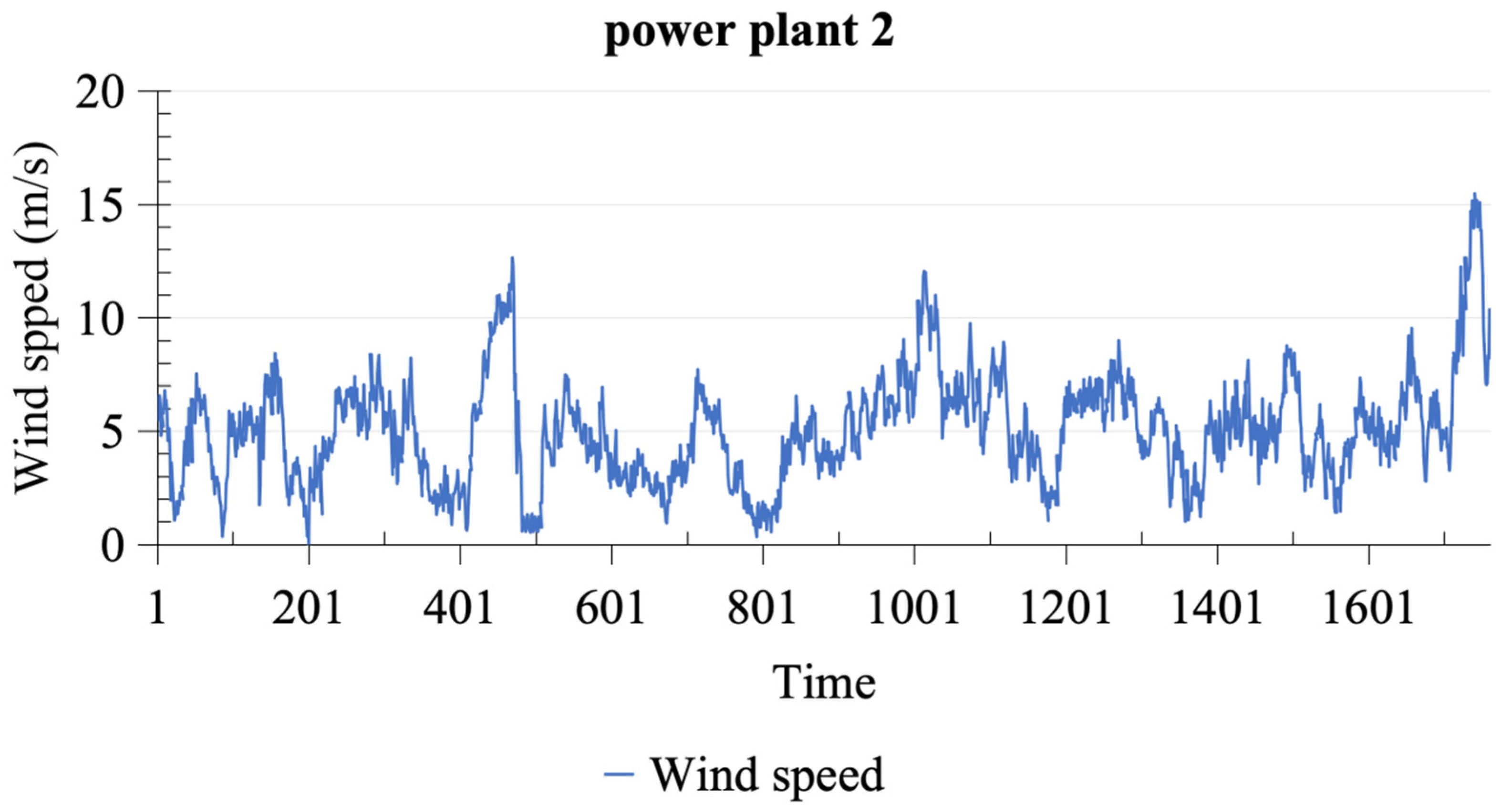
Following a comprehensive assessment of wind speed prediction performance at power plant 2, it becomes evident that deep learning models shine across various critical metrics. Notably, the CNN model emerges as a standout performer in the realm of wind speed prediction, boasting the lowest recorded values for MSE, RMSE, MAE, and MAPE and the highest R 2 , with exceptional scores of 0.0083, 0.0913, 0.0724, 0.4840, and 0.9211, respectively. In addition, both the LSTM and ANN models exhibit commendable performance on the same dataset, characterized by competitive error values, underscoring their significant contributions to enhancing prediction accuracy and stability. In contrast, statistical and machine learning models exhibit relatively subpar performance, marked by higher error values, indicating their diminished predictive accuracy in comparison to their deep learning counterparts.
Taking into consideration the wind speed prediction performance on two different power plants, deep learning models, especially the CNN model, demonstrate outstanding results, with exceptional accuracy and stability. Additionally, the LSTM and ANN models also exhibit a satisfactory performance on the same datasets. In contrast, traditional statistical models perform relatively poorly, with higher errors. This underscores the superior capabilities of deep learning models in handling wind speed data, providing strong support for improving renewable energy efficiency and the reliability of wind power generation.

4. Conclusions and Discussion

4.1. Conclusions

The aim of this study was to compare various types of wind speed time series prediction models, including traditional statistical models (GM and ARIMA), traditional machine learning models (LR, RF, and SVR), and deep learning models (ANN, LSTM, and CNN). Real wind speed data from two different wind power plants were used, and after model training and evaluation, the following conclusions were drawn: (1) Based on the results of this study, deep learning models, particularly the CNN, demonstrated an outstanding performance in wind speed time series prediction, with exceptional accuracy and stability. This finding holds significant implications for the renewable energy industry, especially in the operation and management of wind power plants. Deep learning models exhibit remarkable capabilities in capturing wind speed fluctuations and variations, which are essential for improving the reliability and efficiency of wind energy generation. However, despite the excellent performance of deep learning models, the results of this research also show that traditional deep learning models such as LSTM and ANN perform satisfactorily on the same dataset. This suggests that in practical applications, different types of deep learning models can be chosen based on resource availability and computational capacity. (2) In comparison to deep learning models, traditional statistical models and machine learning models performed less effectively. This may be attributed to the complex nonlinear relationships and time dependencies present in wind speed data, which traditional models struggle to capture. Therefore, in wind speed prediction problems, deep learning models exhibit a distinct advantage. Future research could further explore performance differences among various deep learning models and the impact of parameter tuning to enhance wind speed prediction accuracy.

4.2. Limitations and Future Outlook

This study has two main limitations. First, while the study provides a basic comparison of various time series forecasting models, it does not delve into the detailed optimization of model hyperparameters. This means that the performance of each model could potentially be further improved through fine-tuning of its parameters, and, therefore, a more in-depth hyperparameter optimization process could offer additional insights and opportunities to enhance model performance. Second, the study primarily focuses on the influence of internal factors on wind speed prediction, such as model selection and dataset quality. However, external factors, such as government policies, technological advancements, and changes in the energy market, could also have significant effects on the wind power industry, but these factors were not extensively considered in this study. Hence, in future research, a more thorough exploration of the impact of these external factors on wind speed prediction is needed to gain a more comprehensive understanding.
In future research, there is potential for further enhancing the performance of wind speed prediction models. One potential avenue for improvement is the consideration of ensemble models, which combine various types of models to enhance prediction accuracy. Additionally, a more comprehensive analysis of external factors, such as government policies, technological advancements, and fluctuations in the energy market, should be incorporated into the models to increase the predictability and resilience of the wind energy industry. These additional studies will contribute to making the wind energy sector more reliable and efficient.

Author Contributions

X.L.: Analysis, Software, and Writing. K.L.: Literature, Investigation, Software, Visualization, and Writing. S.S.: Resources and Review. Y.T.: Investigation and Review. All authors have read and agreed to the published version of the manuscript.

Funding

This work was support by the National Natural Science Foundation of China (grant numbers 12301427).

Data Availability Statement

The datasets and materials used in this study are available upon request. Interested researchers can contact Xiangqian Li at [email protected] to request access to the data and materials used in this study.

Acknowledgments

The authors extend their heartfelt appreciation to the reviewers and editors for their invaluable comments and constructive suggestions. Additionally, special thanks go to Marina for providing language help.

Conflicts of Interest

The authors declare that they have no known competing financial interest or personal relationships that could have appeared to influence the work reported in this paper.

Appendix A

Table A1. The parameter settings for the ARIMA model.
ParameterValue
p2
d1
q3
Table A2. The parameter settings for the RF model.
ParameterValue
N_estimators200
Max_depth10
Random_state2
Min_samples_split2
Min_samples_leaf1
BoostrapTrue
CriterionMSE
Table A3. The parameter settings for the SVR model.
ParameterValue
Kernelrbf
C200
Epsilon0.01
Random_state42
Degree3
GammaScale
ShrinkingTrue
Table A4. The parameter settings for the ANN model.
ParameterValue
Lag3
Feature_range(−1, 1)
Input layerNeure: 3
Hidden layer 1Dense layer
Neure: 6
Input_dim: 3
Activation: relu
Hidden layer 2Dense layer
Neure: 6
Input_dim: 6
Activation: relu
Output layerDense layer
Neure: 1
Activation: linear
Loss functionMean squared error loss
OptimizerAdam
Epochs300
Batch size16
Total parameters73
Table A5. The parameter settings for the LSTM model.
ParameterValue
Number of layers3
First layerLSTM layer
Nodes: 50
Activation: relu
Second layerLSTM layer
Nodes: 50
Activation: relu
Third layerDense layer
Nodes: 1
Activation: linear
Loss functionMean squared error loss
OptimizerAdam
Epochs100
Batch size32
Table A6. The parameter settings for the CNN model.
ParameterValue
Look-Back3
Number of Filters32
Kernel Size3
Pooling Window Size1
Activation FunctionRelu
Number of Neurons in Hidden Layer32
OptimizerAdam
Batch Size16
Number of Epochs200
Random_state42
LossMean_squared_error
ModelGMARIMALRRFANNSVRLSTMCNN
Training time(s)0.0670.86330.35633.49356.00840.111353.621362.0818

References

  1. Li, F.; Ren, G.R.; Lee, J. Multi-step wind speed prediction based on turbulence intensity and hybrid deep neural networks. Energy Convers. Manag. 2019, 186, 306–322. [Google Scholar] [CrossRef]
  2. Wang, J.Z.; Guo, H.G.; Li, Z.W.; Song, A.Y.; Niu, X.S. Quantile deep learning model and multi-objective opposition elite marine predator optimization algorithm for wind speed. Appl. Math. Model. 2023, 115, 56–79. [Google Scholar] [CrossRef]
  3. Huang, Y.; Zhang, B.Z.; Pang, H.Z.; Wang, B.; Lee, K.Y.; Xie, J.L.; Jin, Y.P. Spatio-temporal wind speed prediction based on Clayton Copula function with deep learning fusion. Renew. Energy 2022, 192, 526–536. [Google Scholar] [CrossRef]
  4. Zhang, J.W.; Cheng, M.Z.; Cai, X. Short-term Wind Speed Prediction Based on Grey System Theory Modelin the Region of China. Prz. Elektrotechniczny 2012, 88, 67–71. [Google Scholar]
  5. Zhang, Y.G.; Zhao, Y.; Kong, C.H.; Chen, B. A new prediction method based on VMD-PRBF-ARMA-E model considering wind speed characteristic. Energy Convers. Manag. 2020, 203, 112254. [Google Scholar] [CrossRef]
  6. Sim, S.K.; Maass, P.; Lind, P.G. Wind Speed Modeling by Nested ARIMA Processes. Energies 2019, 12, 69. [Google Scholar] [CrossRef]
  7. Ding, W.; Meng, F. Point and interval forecasting for wind speed based on linear component extraction. Appl. Soft. Comput. 2020, 93, 106350. [Google Scholar] [CrossRef]
  8. Zhang, Y.; Sun, H.X.; Guo, Y.J. Wind Power Prediction Based on PSO-SVR and Grey Combination Model. IEEE Access 2019, 7, 136254–136267. [Google Scholar] [CrossRef]
  9. Karakus, O.; Kuruoglu, E.E.; Altinkaya, M.A. One-day ahead wind speed/power prediction based on polynomial autoregressive model. Inst. Eng. Technol. 2017, 11, 1430–1439. [Google Scholar] [CrossRef]
  10. Chen, J.Q.; Xue, X.P.; Ha, M.H.; Yu, D.R.; Ma, L.T. Support Vector Regression Method for Wind Speed PredictionIncorporating Probability Prior Knowledge. Math. Probl. Eng. 2014, 2014, 410489. [Google Scholar] [CrossRef]
  11. Marovic, I.; Susanj, I.; Ozanic, N. Development of ANN Model for Wind Speed Prediction as a Support for Early Warning System. Complexity 2017, 2017, 3418145. [Google Scholar] [CrossRef]
  12. Niu, D.X.; Pu, D.; Dai, S.Y. Ultra-Short-Term Wind-Power Forecasting Based on the Weighted Random Forest Optimized by the Niche Immune Lion Algorithm. Energies 2018, 11, 1098. [Google Scholar] [CrossRef]
  13. Shi, K.P.; Qiao, Y.; Zhao, W.; Wang, Q.; Liu, M.H.; Lu, Z.X. An improved random forest model of short-term wind-power forecasting to enhance accuracy, efficiency, and robustness. Wind Energy 2018, 21, 1383–1394. [Google Scholar] [CrossRef]
  14. Zhang, S.G.; Zhou, T.; Sun, L.; Wang, W.; Wang, C.; Mao, W.T. ν-Support Vector Regression Model Based on Gauss-Laplace Mixture Noise Characteristic for Wind Speed Prediction. Entropy 2019, 21, 1056. [Google Scholar] [CrossRef]
  15. Wei, C.C. Forecasting surface wind speeds over offshore islands near Taiwan during tropical cyclones: Comparisons of data-driven algorithms and parametric wind representations. J. Geophys. Res.-Atmos. 2015, 120, 1826–1847. [Google Scholar] [CrossRef]
  16. Faniband, Y.P.; Shaahid, S.M. Forecasting Wind Speed using Artificial Neural Networks—A Case Study of a Potential Location of Saudi Arabia. E3S Web Conf. 2020, 173, 01004. [Google Scholar] [CrossRef]
  17. Liang, T.; Zhao, Q.; Lv, Q.Z.; Sun, H.X. A novel wind speed prediction strategy based on Bi-LSTM, MOOFADA and transfer learning for centralized control centers. Energy 2021, 230, 120904. [Google Scholar] [CrossRef]
  18. Saeed, A.; Li, C.S.; Danish, M.; Rubaiee, S.; Tang, G.; Gan, Z.H.; Ahmed, A. Hybrid Bidirectional LSTM Model for Short-Term Wind Speed Interval Prediction. IEEE Access 2020, 8, 182283–182294. [Google Scholar] [CrossRef]
  19. Qian, J.C.; Zhu, M.F.; Zhao, Y.N.; He, X.J. Short-term Wind Speed Prediction with a Two-layer Attention-based LSTM. Comput. Syst. Sci. Eng. 2021, 39, 197–209. [Google Scholar] [CrossRef]
  20. Ding, Y.; Ye, X.W.; Guo, Y. A Multistep Direct and Indirect Strategy for Predicting WindDirection Based on the EMD-LSTM Model. Struct. Control. Health Monit. 2023, 2023, 4950487. [Google Scholar] [CrossRef]
  21. Shao, B.L.; Song, D.; Bian, G.Q.; Zhao, Y. Wind Speed Forecast Based on the LSTM Neural Network Optimized by the Firework Algorithm. Adv. Mater. Sci. Eng. 2021, 2021, 4874757. [Google Scholar] [CrossRef]
  22. Geng, D.W.; Zhang, H.F.; Wu, H.Y. Short-Term Wind Speed Prediction Based on Principal Component Analysis and LSTM. Appl. Sci. 2020, 10, 4416. [Google Scholar] [CrossRef]
  23. Lawal, A.; Rehman, S.; Alhems, L.M.; Alam, M.M. Wind Speed Prediction Using Hybrid 1D CNN and BLSTM Network. IEEE Access 2021, 9, 156672–156679. [Google Scholar] [CrossRef]
  24. Raju, H.; Das, S. CNN-Based Deep Learning Model for Solar Wind Forecasting. Solar Phys. 2021, 296, 134. [Google Scholar] [CrossRef]
  25. Arabi, S.; Asgarimehr, M.; Kada, M.; Wickert, J. Hybrid CNN-LSTM Deep Learning for Track-Wise GNSS-R Ocean Wind Speed Retrieval. Remote Sens. 2023, 15, 4169. [Google Scholar] [CrossRef]
  26. Wang, H.K.; Song, K.; Cheng, Y. A Hybrid Forecasting Model Based on CNN and Informer for Short-Term Wind Power. Comput. Intell. Neurosci. 2021, 9, 788320. [Google Scholar] [CrossRef]
  27. Upendran, V.; Cheung, M.C.M.; Hanasoge, S.; Krishnamurthi, G. Solar Wind Prediction Using Deep Learning. Space Weather 2020, 18, e2020SW002478. [Google Scholar] [CrossRef]
  28. Wu, W.Q.; Ma, X.; Zhang, Y.Y.; Li, W.P.; Wang, Y. A novel conformable fractional non-homogeneous grey model for forecasting carbon dioxide emissions of BRICS countries. Sci. Total Environ. 2020, 707, 135447. [Google Scholar] [CrossRef]
  29. Jian, L.; Zhao, Y.; Zhu, Y.P.; Zhang, M.B.; Bertolatti, D. An application of ARIMA model to predict submicrion particleconcentrations from meteorological factors at a busy roadside in Hangzhou, China. Sci. Total Environ. 2012, 426, 336–345. [Google Scholar] [CrossRef]
  30. Jeong, J.I.; Park, R.J.; Yeh, S.W.; Roh, J.W. Statistical predictability of wintertime PM2.5 concentrations over East Asia using simple linear regression. Sci. Total Environ. 2021, 776, 146059. [Google Scholar] [CrossRef]
  31. Zhao, Z.Y.; Xiao, N.W.; Shen, M.; Li, J.S. Comparison between optimized MaxEnt and random forest modeling in predicting potential distribution: A case study with Quasipaa boulengeri in China. Sci. Total Environ. 2022, 842, 156867. [Google Scholar] [CrossRef]
  32. An, Y.F.; Zhai, X.Q. SVR-DEA model of carbon tax pricing for China’s thermal power industry. Sci. Total Environ. 2020, 734, 139438. [Google Scholar] [CrossRef]
  33. Almomani, F. Prediction the performance of multistage moving bed biological process using artifical neural network (ANN). Sci. Total Environ. 2020, 744, 140854. [Google Scholar] [CrossRef]
  34. Yokoo, K.; Ishida, K.; Ercan, A.; Tu, T.B.; Nagasato, T.; Kiyama, M.; Amagasaki, M. Capabilities of deep learning models on learning physical relationships: Case of rainfall-runoff modeling with LSTM. Sci. Total Environ. 2021, 802, 149876. [Google Scholar] [CrossRef]
  35. Faraji, M.; Nadi, S.; Ghaffarpasand, O.; Homayoni, S.; Downey, K. An integrated 3D CNN-GRU deep learning method for short-term prediction of PM2.5 concentration in urban environment. Sci. Total Environ. 2022, 834, 155324. [Google Scholar] [CrossRef]
  36. Shen, Q.Q.; Wang, G.Y.; Wang, Y.H.; Zeng, B.S.; Yu, X.; He, S.C. Prediction Model for Transient NOx Emission of Diesel Engine Based onCNN-LSTM Network. Energies 2023, 16, 5347. [Google Scholar] [CrossRef]
  37. Moez, K. Convolutional Neural Networks: A Survey. Computers 2023, 12, 151. [Google Scholar] [CrossRef]
  38. Fahad, A.; Arshi, N.; Hamed, A. E-Learning modeling technique and convolution neural networks in online education. In IoT-Enabled Convolutional Neural Networks: Techniques and Applications; River Publishers: Aalborg, Denmark, 2023; Volume 35, ISBN 9781003393030. [Google Scholar]
  39. Gaba, S.; Budhiraja, I.; Kumar, V.; Garg, S.; Kaddoum, G.; Hassan, M.M. A federated calibration scheme for convolutional neural networks: Models, applications and challenges. Comput. Commun. 2022, 192, 144–162. [Google Scholar] [CrossRef]
  40. Pavicevic, M.; Popovic, T. Forecasting day-ahead electricity metrics with artificial neural networks. Sensors 2022, 22, 1051. [Google Scholar] [CrossRef]
  41. Zhang, Y.; Wu, H.; Xu, R.; Wang, Y.P.; Wei, C.H. Machine learning modeling for the prediction of phosphorus and nitrogen removal efficiency and screening of crucial microorganisms in wastewater treatment plants. Sci. Total Environ. 2023, 907, 167730. [Google Scholar] [CrossRef]
  42. Lu, S.Y.; Zhang, B.Q.; Ma, L.F.; Xu, H.; Li, Y.T.; Yang, S.B. Economic load-reduction strategy of central air conditioning based on convolutional neural network and pre-cooling. Energies 2023, 16, 5035. [Google Scholar] [CrossRef]
Figure 1. Research framework diagram.
Energies 16 07785 g001
Figure 2. The structure of the RF model.
Energies 16 07785 g002
Figure 3. ANN model diagram.
Energies 16 07785 g003
Figure 4. LSTM model diagram.
Energies 16 07785 g004
Figure 5. Diagram of the CNN model framework.
Energies 16 07785 g005
Figure 6. The wind speed dataset collected in power plant 1.
Energies 16 07785 g006
Figure 7. The wind speed dataset collected in power plant 2.
Energies 16 07785 g007
Table 1. Summary statistics of experimental data.
SumMeanMaxMinVarianceMedianKurtSkew
Power 117614.5712.6105.104.290.340.74
Power 217615.0615.480.015.654.981.700.82
Table 2. Model performance comparison for power plant 1.
Power Plant 1
Statistical ModelMachine Learning ModelDeep Learning Model
GMARIMALRRFSVRANNLSTMCNN
MSE0.16690.25334.80170.01610.53350.01440.01360.0124
RMSE0.40850.50332.19130.12710.73040.12030.11670.1112
MAE0.33260.42841.77750.09580.53700.09160.08910.0855
MAPE3.88041.86690.65420.98560.14260.12391.15080.7688
R2−0.0128−0.42190.05540.90980.88850.91660.92400.9274
Table 3. Model performance comparison for power plant 2.
Power Plant 2
Statistical ModelMachine Learning ModelDeep Learning Model
GMARIMALRRFSVRANNLSTMCNN
MSE0.09360.15445.68850.02351.08130.01480.01200.0083
RMSE0.30590.39302.38510.15331.03990.12170.10970.0913
MAE0.22570.25641.79790.10550.64570.09170.08610.0724
MAPE2.78422.35680.56480.65140.50080.54960.60480.4840
R2−0.0292−0.26690.08090.80830.82870.87540.90190.9211
Disclaimer/Publisher’s Note: The statements, opinions and data contained in all publications are solely those of the individual author(s) and contributor(s) and not of MDPI and/or the editor(s). MDPI and/or the editor(s) disclaim responsibility for any injury to people or property resulting from any ideas, methods, instructions or products referred to in the content.

