Article

Optimized Dispatch of Regional Integrated Energy System Considering Wind Power Consumption in Low-Temperature Environment

College of Electrical Engineering and New Energy, China Three Gorges University, Yichang 443002, China
*
Author to whom correspondence should be addressed.
Energies 2023, 16(23), 7791; https://doi.org/10.3390/en16237791
Submission received: 5 November 2023 / Revised: 20 November 2023 / Accepted: 24 November 2023 / Published: 27 November 2023

Abstract

:
The wind abandonment phenomenon of cogeneration units in regional integrated energy systems (RIES) under the operation mode of “heat for electricity” and the improvement in the operation efficiency of the energy storage system under a low-temperature environment are problems that need to be solved urgently. To this end, a regional integrated energy system optimization scheduling method based on fine energy storage and wind power consumption is proposed in the paper. First, a fine energy storage model more adapted to a low-temperature environment is established on the power side to accurately simulate the actual working state of the energy storage components and quantify the uncertainty of the wind power output using the conditional value-at-risk (CVaR) theory. Then, a combined heat and power demand response mechanism is introduced on the load side to reduce the peak-to-valley difference in the heat and power loads, it is realized to promote the system’s consumption of wind power without increasing the transmission power of the contact line. Finally, the example is solved on the MATLAB platform with the objective of minimizing the total cost of the RIES optimal dispatch. The simulation results show that the proposed model is not only more adaptable to a low-temperature environment compared with the traditional model but also reduces the overall cost of the system by 2.58% while realizing the complete consumption of wind power. This innovative study provides a feasible and efficient solution to improve the performance of integrated energy systems, especially the operation capability in extreme environments.

1. Introduction

With the intensification of the energy crisis, increasing the utilization rate of renewable energy and reducing fossil energy dependence has become an important research direction. Integrated regional energy systems have rapidly developed as an effective way to increase the utilization of renewable energy and reduce pollutant emissions [1]. Cogeneration units centered on combined heat and power (CHP) technology are capable of generating both electricity and heat and are used in a wide range of applications. As CHP units are often in heat-determined power operation in winter, the heat load is at its peak during the nighttime when the electric load is in the trough, and the system peaking capacity is smaller than that of conventional units, making it more prone to the phenomenon of wind abandonment [2].
In integrated energy systems, energy storage devices change the load distribution in the spatial and temporal dimensions to improve system stability and economics. One study [3] verified the effect of a ground source heat pump and energy storage device on the system’s economy based on the RIES optimal scheduling model containing a ground source heat pump and energy storage, but it lacked a more in-depth study on the operational characteristics of the energy storage device. Another study [4], based on the characteristics of multi-energy coupling and energy conversion of cold, heat, electricity, and gas, combined with the energy storage characteristics of the system, put forward the optimal scheduling method based on the RIES of the day but failed to take into account the impact of load fluctuations on the operation of the RIES. Other researchers [5] analyzed the energy storage capacity and economic benefits of RIES from the perspective of integrated demand response and uncertainty but failed to consider the impact of the idiosyncrasy of the energy storage system under different ambient temperatures on the optimal scheduling. Two studies [6,7] proposed the possibility of using shared energy storage instead of traditional energy storage to achieve low-cost wind power consumption, but the uncertainty of the effective capacity of the shared energy storage system makes it difficult to effectively consume wind power. [8] proposes an integrated electricity and heat system, which can significantly improve the energy utilization rate under the regulation of distributed management strategy, but the lack of analysis of heat loss from heat storage tanks in low-temperature environments will lead to a large discrepancy between the scheduling results and the actual situation. However, none of the above studies takes into account the differences in the characteristics of the energy storage devices in the RIES, such as the effect of charging and discharging power of the battery at low temperatures and the effect of the heat loss of the thermal storage tanks by the ambient temperature. Therefore, it is particularly important to consider the characteristics of energy storage devices under low temperatures and other conditions for accurate scheduling of integrated energy systems.
The RIES addresses the phenomena of wind energy output uncertainty and large differences in load peaks and valleys on the source and load side, which lead to the problems of impeded wind energy consumption and a high integrated cost of dispatch. On the energy supply side, the current mainstream methods for dealing with the wind energy uncertainty problem include stochastic optimization and robust optimization. [9] coordinates the robustness and economy of the system by flexibly adjusting the robust parameters to improve the system’s level of wind power consumption, but effectively fails to address the shortcoming that the robust optimization results are biased towards conservatism. Others [10,11] established a stochastic optimization model of an integrated energy system with electric vehicles and simulated the wind power output based on the scenario reduction technique with improved probability distance, which improved the accuracy of the scheduling results, but the stochastic optimization can easily fall into the local optimal solution, which makes the optimization results lack credibility. Other research [12,13] proposed to use the conditional value at risk (CVaR) theory to deal with the uncertainty set to obtain a more economically efficient optimization scheme, in view of the fact that robust optimization is only affected by the worst-case scenarios of the uncertain input parameters, and the final results obtained are too conservative. On the energy demand side, [14] establishes a demand response optimization model based on electricity price (based on RIES demand-side characteristics), but fails to consider the demand response mechanism of thermal loads, which has limited capacity for wind power consumption. Another study [15] established an integrated energy system containing electricity to gas and energy storage devices based on gas–electricity joint demand response and established a demand response optimization model based on electricity price based on RIES energy demand-side characteristics. [16] established an integrated energy system economic dispatch model with integrated demand response (IDR) for combined heat and power with the objective of minimizing wind abandonment rate. However, these studies consider only the impact of source-side or load-side characteristics on system operation and do not consider the source and load sides together. [17] comprehensively considered the impact of source- and load-side characteristics on wind power consumption and effectively improved wind power consumption by integrating high-penetration wind energy through interconnecting lines but did not consider how to effectively consume wind power when the transmission power of the contact line could not meet the demand.
Aiming at the above problems, this paper proposes a coordinated optimization model of RIES based on fine energy storage and wind power consumption. Firstly, a fine energy storage model more in line with a low-temperature environment is established, and consideration is given to increasing the thermal load to safeguard the available capacity of the storage battery and the charge/discharge speed and improve the utilization rate of the energy storage system. Secondly, to address the uncertainty of wind power output on the energy supply side, the Latin hypercube–synchronous back-generation elimination method is used to obtain more accurate wind power output based on the historical data of wind power output, and the CVaR theory is used to quantify the risk of revenue and enhance the system’s ability to consume wind power. At the same time, the introduction of a heat and power demand response mechanism on the load side cuts down the peak-to-valley difference in the system load and further improves the system’s level of wind power consumption. After comprehensively considering the energy conversion characteristics of the source and load sides and the operation characteristics of the energy storage device, the model is solved using MATLAB 2018b to obtain the wind abandonment rate and operation scheme under the lowest operation cost. The example results show that compared with the traditional model, the RIES model based on fine energy storage and wind power consumption can effectively improve the level of wind power consumption and reduce the operating cost of the system.

2. Integrated Energy System Architecture

Due to the cold winter climate in the north, there is a high demand for heating. At the same time, the region is rich in geothermal energy, wind energy, solar energy, and other renewable energy sources, which provide a good foundation for the application of ground source heat pumps and CHP in the region [18,19]. Compared with the traditional RIES, which is limited to the independent operation of a single form of energy, this paper establishes a RIES containing integrated energy storage (IES) equipment, wind turbines (WT), photovoltaic (PV), ground source heat pumps (GSHP), and CHP units, with the structure shown in Figure 1, which can utilize and synergize the outputs of different forms of energy in a more effective way. The power load demand is met by the superior grid, wind turbines, photovoltaic power plants, and cogeneration units; the heat load demand is met by the cogeneration units and ground source heat pumps, and the energy storage equipment includes a heat storage tank (HST) and an IES to provide support for the heat and power loads. Considering that the actual available capacity of the IES is greatly affected by the temperature in winter, the working efficiency of the IES is guaranteed by increasing part of the thermal load.

2.1. CHP System

CHP systems are capable of delivering both heat and power at the same time. They convert high-quality heat from the combustion of natural gas into electricity and absorb the waste heat to meet the heat load by using a bromine chiller; it usually consists of a bromine chiller (BC) and a gas turbine (GT) [20] and is mathematically modeled as follows:
P B , h ( t ) = Q G ( t ) δ B λ B , h
Q G ( t ) = P G T ( t ) ( 1 β G β l ) / β G
where P B , h ( t ) , P G T ( t ) , and Q G ( t ) represent the heating power of the BC and the electric power output and waste heat generated by the GT at the moment t, respectively; δ B , λ B , h , βG, and βl are, in order, the recovery rate of the flue gas of the BC, the heat production coefficient of the flue gas of the BC, the power generation efficiency of the GT, and the heat loss coefficient of the GT.

2.2. Ground Source Heat Pump

Compared with traditional heating equipment such as electric boilers, a ground source heat pump converts a large number of low-temperature heat sources in the shallow ground into high-quality energy to meet heating and cooling needs with a small electrical energy input. The mathematical model for its heat supply is as follows:
P GH ( t ) = λ l P GHI ( t )
where P GH ( t ) and P GHI ( t ) are the heating power and power consumption of the GSHP at the moment t , respectively; λ l is its heating efficiency.

2.3. Fine Energy Storage Equipment

As an important component of the RIES, energy storage equipment mainly includes thermal storage tanks and batteries. These devices absorb and release energy, thus reducing system fluctuations, especially suppressing fluctuations due to the uncertainty of new energy output. The charging and discharging mathematical model of the energy storage system is as follows:
S IES ( t ) = ( 1 η IES ) S IES ( t 1 ) + ( M P in ( t ) λ in Δ t N P out ( t ) λ out Δ t )
M + N 1 ,   M { 0 , 1 } ,   N { 0 , 1 }
where S IES ( t ) is the remaining energy of the energy storage device at time t ; P in ( t ) and P out ( t ) represent the energy input and output power of the energy storage device at time t, respectively; λ in and λ out represent the conversion efficiencies of the energy input and output of the energy storage device, respectively; M and N are Boolean variables that represent the state of the energy storage device, which is in a state of charging at M = 1 and in a state of energy release at N = 1; and η IES is the energy loss coefficient of the energy storage device.

2.3.1. Battery Storage Model

The traditional energy storage model does not consider the effect of ambient temperature on the battery, but the actual usable capacity is related to the surface temperature of the battery [21,22], which is mathematically expressed as follows:
S IESN ( t ) = S EIESN [ 1 + ξ a ( T a ( t ) T N ) ]
where S EIESN represents the standard state of the rated capacity of the battery; T a ( t ) is the battery surface temperature at the moment of t; and T N is the standard state of the temperature, T N taking the value of 25 °C.
The surface temperature of the battery is determined by its heat generation and heat dissipation during the working period, and its mathematical expression is as follows:
T a ( t ) = T a ( t 1 ) + Φ in ( t ) Φ out ( t ) K tep S ele Φ in , e ( t ) = λ IES [ M ele · P IES , in ( t ) + N ele · P IES , out ( t ) ] Δ t Φ out , e ( t ) = K tep S ele ( T a ( t 1 ) T evr ( t ) )
where Φ in , e ( t ) and Φ out , e ( t ) are the heat generation and dissipation of the battery at the moment of t; P IES , in ( t ) and P IES , out ( t ) are the charging and discharging power of the battery at the moment of t; M ele and N ele indicate the working state of the battery: M ele = 1 when the battery is in the charging state, N ele = 1 when the battery is in the discharging state; T evr ( t ) represents the ambient temperature at the moment of t; ξ a is the capacity temperature coefficient; S ele is the surface area of the battery; K tep is the heat convection coefficient; λ IES is the battery heat generation coefficient.
In addition, the service life of the battery is also affected by its charging and discharging rate. If the charge/discharge rate is too high, the service life will be seriously damaged. Therefore, the maximum charging and discharging power per hour should be limited to not more than 20% of the actual usable capacity [23], and its mathematical model is as follows:
P IES , in ( t ) 0.2 S IESN ( t ) / Δ t P IES , out ( t ) 0.2 S IESN ( t ) / Δ t
In order to improve the utilization of the battery in practical applications, this paper optimizes the problems that may occur in the energy storage process. Specific measures include the rational design of battery charging and discharging programs and artificially increasing the ambient temperature to increase the actual available capacity.

2.3.2. Model of Heat Storage Tank

The heat storage tank model consists of an atmospheric pressure hot water storage tank, a circulating pump, and additional equipment such as a heat exchanger. In practice, due to the influence of the ambient temperature, there is a certain amount of heat loss in the heat storage tank, mainly the inner wall of the tank to transfer heat and the outer surface of the tank to the surrounding air to emit heat [24,25]. The mathematical model of the heat storage tank storage and heat release is as follows:
S LES ( t ) = η wat m T LES ( t ) T LES ( t ) = T LES ( t 1 ) + Φ in , w ( t ) Φ out , w ( t ) K wat S wat Φ in , w ( t ) = H dis ( t ) ω dis H ch ( t ) ω ch Δ t Φ out , w ( t ) = K wat S wat ( T LES ( t 1 ) T evr ( t ) )
where S LES ( t ) is the heat storage capacity of the heat storage tank at time t; η wat is the specific heat capacity of water; m is the mass of hot water in the heat storage tank; K wat and S wat are the integrated thermal convection coefficient and surface area of the heat storage tank, respectively; Φ in , w ( t ) and Φ out , w ( t ) are the heat input and heat loss from the heat storage tank, respectively; H ch ( t ) and H dis ( t ) are the storage and discharge thermal power of the heat storage tank, respectively; and ω ch and ω dis are the storage and discharge efficiencies of the heat storage tank, respectively.

3. Combined Heat and Power Demand Response Mechanism

3.1. Electric Load Demand Response

A price-based DR (PBDR) model is established based on the price-based demand response mechanism. Through PBDR, the demand side electricity consumption is regulated to effectively realize peak shifting and valley filling and to reduce the peak pressure of the system [26,27]. The demand elasticity of the consumer load is as follows:
M t 1 , t 2 = Δ K t 1 K 0 t 1 C 0 t 2 Δ C t 2 M t 1 , t 2 0 , t 1 t 2 M t 1 , t 2 0 , t 1 = t 2
where K 0 t 1 is the amount of electric load at t1 before taking demand response; Δ K t 1 is the change of electric load at t1 after taking demand response; C 0 t 2 is the electric price at t2 before taking demand response; Δ C t 2 is the change of electric price at t2 after taking demand response; M t 1 , t 2 is the cross-elasticity coefficient when t 1 t 2 ; and M t 1 , t 2 is the self-elasticity coefficient when t 1 = t 2 . After the introduction of the PBDR model, the change amount in electric load is as follows:
  Δ K 1 / K 0 1   Δ K 2 / K 0 2 Δ K 24 / K 0 24 = M 11   M 124 M 21   M 224   M 241   M 2424 Δ C 1 / C 0 1 Δ C 2 / C 0 2   Δ C 24 / C 0 24
With the introduction of the PBDR model, the magnitude of the electrical load at time t is as follows:
K load , e t = K 0 t ( 1 + Δ K t / K 0 t )

3.2. Heat Load Demand Response

The heat load of a residential area consists of two parts: domestic hot water and heating heat load. The heating heat load is more elastic and accounts for a higher proportion of the total heat load, while domestic hot water is a rigid load with little change and accounts for a smaller proportion of the total heat load. In order to accurately assess the impact of heat load on wind power consumption, we only analyzes and calculates the heating heat load [28]. The current outdoor temperature and the expression for the relationship between the required thermal power and the amount of change in the indoor temperature of the house are as follows:
P l , h ( t ) = N 0 R ( T i ( t + 1 ) e Δ t / τ T i ( t ) 1 e Δ t / η T o ( t ) ) η = R C 0
where P l , h ( t ) represents the thermal power required in the room at the moment t; N 0 is the number of heating households in the residential area; C 0 is the air heat capacity in the room; R is the equivalent thermal impedance of the house; and T i ( t ) and T o ( t ) are the indoor and outdoor temperatures of the house at the moment t .
Due to the human body’s ambiguity in perceiving temperature changes in the surrounding environment, when the indoor temperature changes within a slow and small range, it does not cause discomfort. In order to assess the degree of living comfort, [29] used the predicted mean vote (PMV) as a quantitative indicator. This research states that when γ PMV is between −0.5 and 0.5, the comfort level of the inhabitants is not affected. Based on the above, the constraints on indoor temperature are as follows:
T i , min T i ( t ) T i , max
where T i , max and T i , min are the maximum and minimum indoor temperatures, respectively.

4. Scenario Selection and CVaR Theory

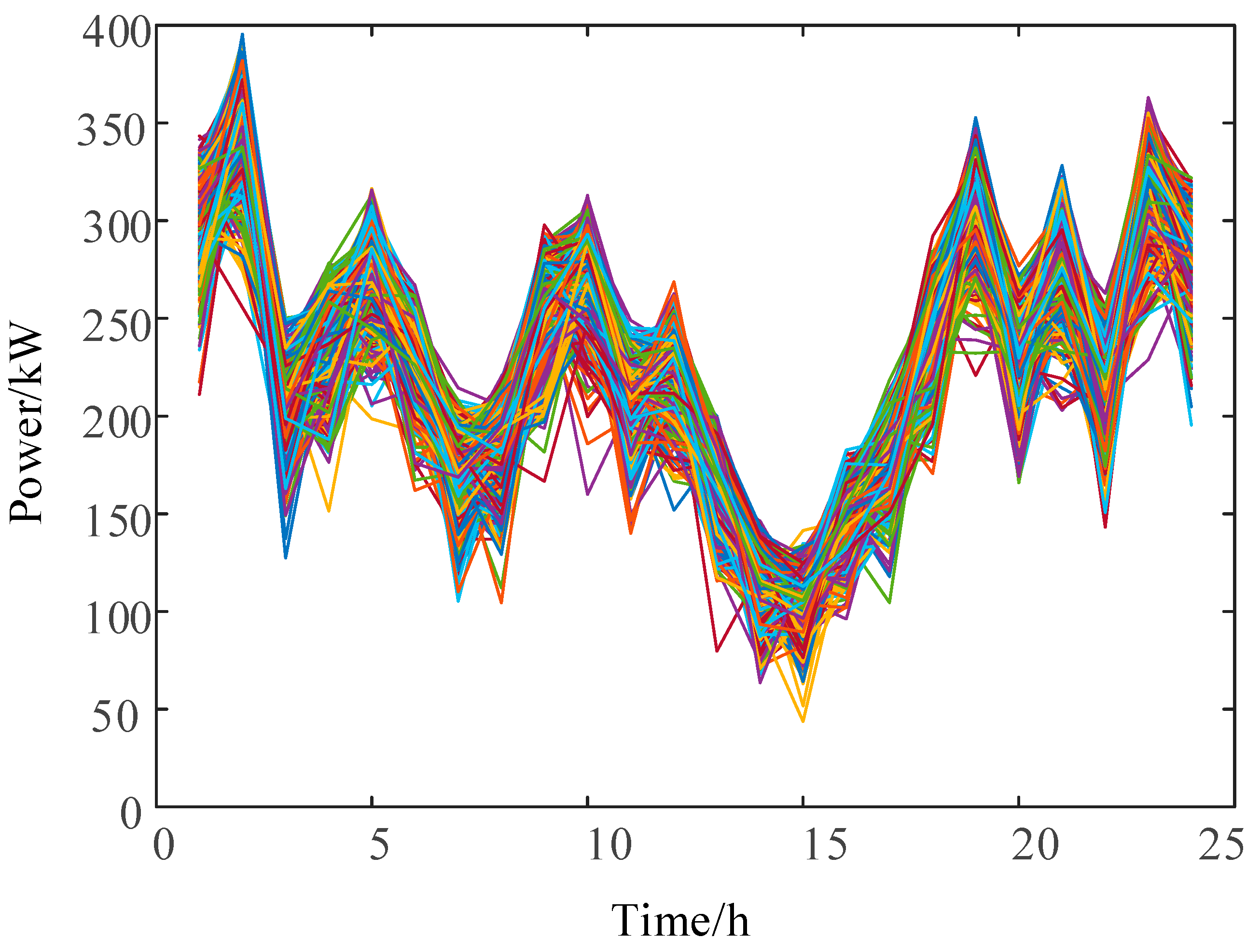
4.1. Uncertain Scenario Selection

In this paper, using historical wind power output data, the kernel density estimation method is used to establish the actual probability density distribution function of the prediction error of wind power output at each scheduling moment, and Latin hypercubic sampling is applied to obtain the set of prediction error samples at each scheduling time point of the system [30]. In order to improve computational efficiency, this paper adopts the synchronized back-generation elimination method to cut down the scenario s and get the corresponding probability values. Let the set of scenario s be W s = W s , 0 , W s , 1 , W s , t , W s , T , where W s , t is the outgoing value of scenario s at time t, and the sum of the probability of occurrence of each scenario is 1. The expressions for the distances between the different scenarios are as follows:
D ( W s , W j ) = [ t = 1 T ( W s ( t ) W j ( t ) ) 2 ] 1 2
In order to make the sample set better approximate the original scenario set, the paper adopts the scenario -cutting technique to obtain multiple scenario sets with corresponding probabilities by clustering similar scenarios. At the same time, it is also necessary to satisfy the minimization of the probability distance between the cut scenario sets. The mathematical expression is as follows:
min s J , j J T D ( W s , W j )

4.2. CVaR Overview

CVaR is developed from value at risk (VaR), which represents the worst possible loss that a portfolio can suffer at a certain confidence level [31]. Specifically, assuming that the decision variable is u, the uncertainty variable is v, and its probability density function is R ( v ) , the loss function of u is S ( u , v ) . Then, when u is fixed, the loss function S ( u , v ) does not exceed the cumulative distribution function at threshold θ , as follows:
π ( u , θ ) = S ( u , v ) θ R ( v ) d v
At a specific confidence level, α , VaR represents the maximum loss of revenue that the RIES may face in a future dispatch cycle, which is mathematically modeled as follows:
f VaR ( u ) = min { θ : π ( u , v ) α }
CVaR is a measure of the average return loss of the RIES in the event that a given VaR value is exceeded in the system return. Its mathematical model can be expressed as follows:
f CVaR ( u ) = 1 1 α S u , v f VAR ( u ) S ( u , v ) R ( v ) d v
Considering that it is difficult to calculate CVaR directly from Equation (19), [32] proposes a simple calculation method as follows:
f CVaR ( u ) = min θ + 1 1 α S = 1 S max { S u , v θ , 0

5. RIES Coordinated Optimization Model Considering CVaR

5.1. Objective Function

Due to the uncertainty of wind turbine output, there is a potential risk in the economic dispatch scheme. In order to comprehensively consider the performance of the model in different operating environments, this paper adopts the conditional value at risk (CVaR) to quantify the risk of returns in various situations [33,34]. The RIES coordination optimization model is established with the objective function of minimizing the total cost of the RIES operation, which is shown as follows:
min f = β f EX + ( 1 β ) f CVaR f EX = S = 1 S P S f S f CVaR ( x ) = θ + 1 1 α S = 1 S P S · max { f S θ , 0 } f S = t = 1 T C w S ( t ) + C grid S ( t ) + C e S ( t ) + C fu S ( t ) + C wt S ( t )
where f is the total economic cost of system operation; f CVaR is the CVaR cost; f EX is the expected cost; θ is the auxiliary variable; α is the confidence level; β is the weighting coefficient; P S is the corresponding probability of Scenario S; S is the number of scenarios; T is the period of scheduling; and C w S t , C grid S t , C e S t , C fu S t , and C wt S t are the operation and maintenance (O&M) cost, the cost of power interaction with the superior grid, the cost of environmental cost with the superior grid, the cost of gas purchased with the superior grid, and the cost of wind abandonment with the superior grid, at the time t under Scenario S , respectively.
  • O&M costs
The O&M costs consist of the operation and maintenance costs of controllable units, new energy units, and energy storage equipment, which are expressed as follows:
C w S ( t ) = i = 1 K P a S ( t ) W a + j = 1 N 1 P b S ( t ) W b + n = 1 N 2 P ES , n S ( t ) W n
where P a S ( t ) and P b S ( t ) are the output power per unit O&M cost of the controllable unit, a, and renewable energy machine, b, at moment t under Scenario S , respectively; P ES , n S ( t ) is the transmission power per unit O&M cost of energy storage device n at moment t under Scenario S , and W a , W b , W n are the unit O&M cost per unit of controllable unit a, renewable energy machine b, and energy storage device n at moment t under Scenario S , respectively.
  • Electricity Interaction Costs
The cost of electricity interaction represents the sum of the cost of electricity purchased by the RIES from the main grid and the benefit of electricity sold to the main grid, expressed as follows:
C grid S ( t ) = L g ( t ) max { P d S ( t ) , 0 } L s ( t ) · max { P d S ( t ) , 0 }
where L g ( t ) and L s ( t ) represent the prices at which the grid makes power purchases and sells power at moment, respectively; P d S ( t ) denotes the power on the contact line of the grid at moment t under Scenario S , which is greater than 0 for power purchases and less than 0 for power sales.
  • Environmental costs
The environmental costs represent the GHG emissions emitted during the operation of the controllable units and the GHG treatment costs caused by purchasing electricity from the main grid, which are specified as follows:
C e S ( t ) = m = 1 M λ m [ E m P a S ( t ) + E m P d , b S ( t ) ]
where P d , b S ( t ) is the power purchased by the system at moment t under Scenario S ; E m and λ m are the share coefficient of the m th greenhouse gas and the treatment cost, respectively; and M is the type of greenhouse gas.
  • Wind abandonment costs
The cost of maintaining the wind turbine system during the period of wind abandonment is the cost of wind abandonment, which is expressed as follows:
C wt S ( t ) = P wt S ( t ) D wt
where P wt S ( t ) and D wt are the abandoned wind power and unit abandoned wind cost at moment t under Scenario S , respectively.
  • Cost of gas purchases
The cost of purchasing gas for the CHP system can be expressed as follows:
C fu S ( t ) = P a S ( t ) β G Δ t L CH 4 D CH 4
where L CH 4 and D CH 4 are the average calorific value and gas price of the gas, respectively.

5.2. Restrictive Condition

Considering the operating parameters of the various devices, the RIES needs to satisfy the following constraints.
  • Electrical and thermal power balance constraints:
K load , e ( t ) + P lh S ( t ) = P GT S ( t ) + P WT S ( t ) + P d S ( t ) + P PV S ( t ) + P IES S ( t ) P l , h S ( t ) = P BC , h S ( t ) + P lp , h S ( t ) + H in S ( t )
where K load , e ( t ) and P l , h S ( t ) are the power of the system’s electrical and thermal loads, respectively.
  • Controllable unit operating constraints:
P a , min P a S ( t ) P a , max λ i , min Δ t P a S ( t ) P a S ( t 1 ) λ i , max Δ t
where λ i , max and λ i , min are the upper and lower limits of the climbing rate of controllable unit i, respectively; and P a , max and P a , min are the upper and lower limits of the output force of controllable unit a, respectively.
  • Interactive power constraints with the higher grid:
P d , min P d S ( t ) P d , max
where P d , max and P d , min are the maximum and minimum values of grid interaction power.
  • Wind power output constraints:
0 P WT S ( t ) P ut S ( t ) P WT S ( t ) P ut S ( t ) h ut
where P WT S ( t ) and P ut S ( t ) denote the actual and predicted power of wind power at moment t under Scenario S, respectively, and h ut is the minimum rate of wind power consumption.
  • Energy storage device constraints
P min S ( t ) P IES S ( t ) P max S ( t ) E min S ( t ) E IES S ( t ) E max S ( t ) E IES S ( 0 ) = E IES S ( 24 )
where P max S ( t ) and P min S ( t ) are the maximum and minimum values of the transmission power of the energy storage device at moment t under Scenario S within the constraints; E max S ( t ) and E min S ( t ) are the maximum and minimum available energy storage capacity of the energy storage device at moment t under Scenario S.
  • Electric load demand response constraints
t = 1 24 K up S ( t ) = t = 1 24 K down S ( t ) 0 K up S ( t ) δ up · K load , e ( t ) 0 K up S ( t ) δ down · K load , e ( t )
where K up S ( t ) and K down S ( t ) denote the amount of load transfer in and out at moment t under Scenario S , respectively; and δ up and δ down are the proportions of the maximum upward and maximum downward load transfers, respectively.

6. Calculus Analysis

6.1. Parameterization

In order to verify the RIES model in the paper in terms of the economy of system operation and scheduling and the timeliness of wind power consumption, the paper sets up the simulation of the RIES coordinated optimization model in the following four scenarios for verification. Scenario 1 is the traditional RIES model, without considering demand response and battery heating; Scenario 2 is the RIES model with fine energy storage, without considering demand response and battery heating; Scenario 3 is the RIES model with fine energy storage, considering demand response and battery heating; and Scenario 4 is the RIES model with fine energy storage, which considers both demand response and battery heating. Scenario 4 is the model proposed in the paper. The model parameters are taken as confidence level α = 0.85 and weighting factor β = 0.9. The parameters of the energy storage system are shown in Table 1, and the pollutant treatment cost and unit operation parameters are shown in Table 2 and Table 3. The forecast data of PV, wind power, and electric heat loads are shown in Figure 2, and the temperature and the purchase and sale price of electricity are shown in Figure 3. Taking the economy of system optimization operation and the timeliness of wind power consumption as the goal, the MATLAB platform is used to build the RIES coordinated optimization operation model and the CPLEX solver to solve the model.
We introduce the Latin hypercubic sampling method to deal with the uncertainty introduced by wind power output. The method can quickly generate one thousand typical wind power scenarios and reduce them to five typical scenarios by synchronized back-generation elimination. Its sample space and reduced scenarios are shown in Figure 4 and Figure 5, and the probability sum after the reduced scenarios is 1. It is assumed that the wind turbine output day-ahead prediction error is within 20%.

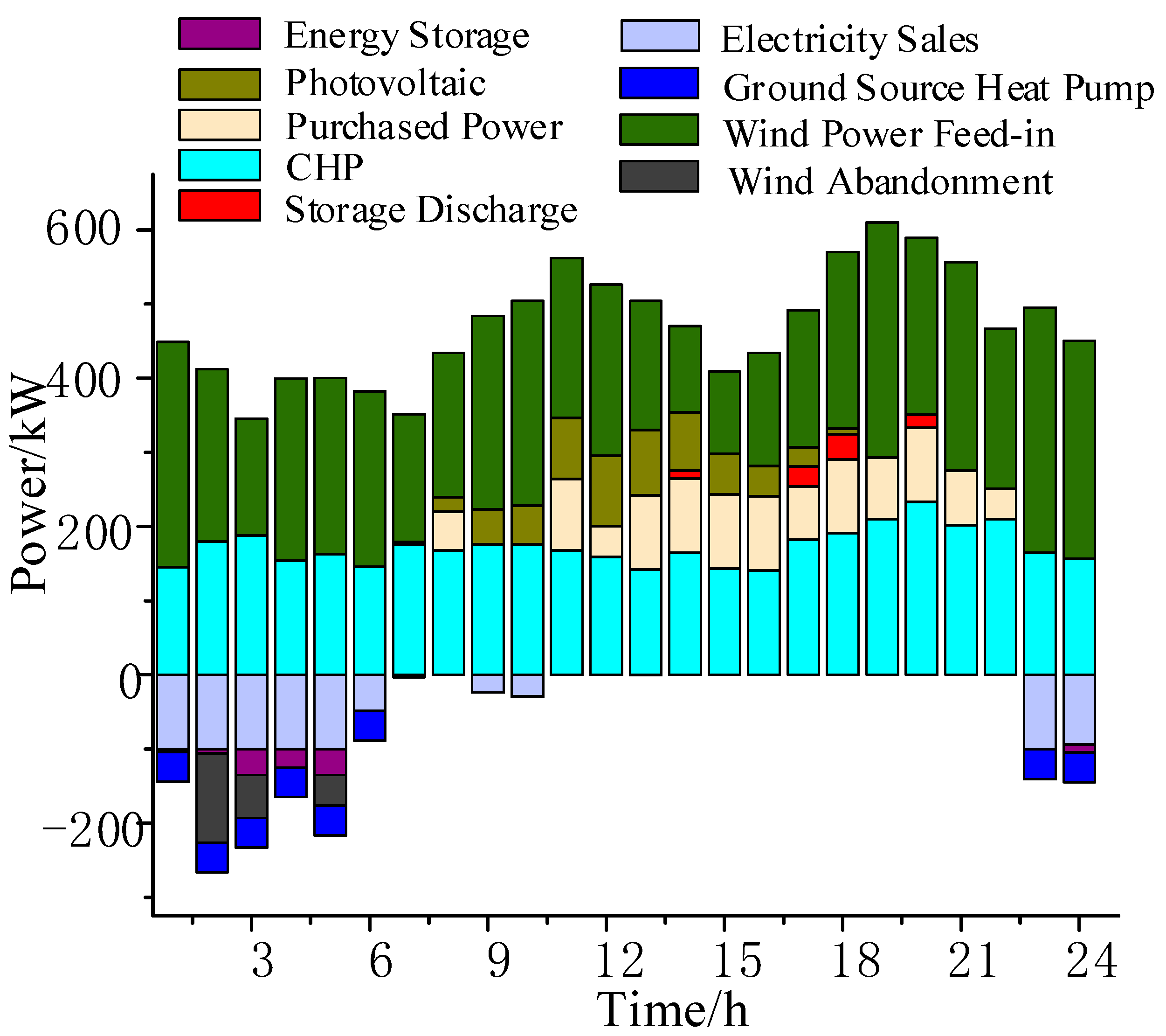
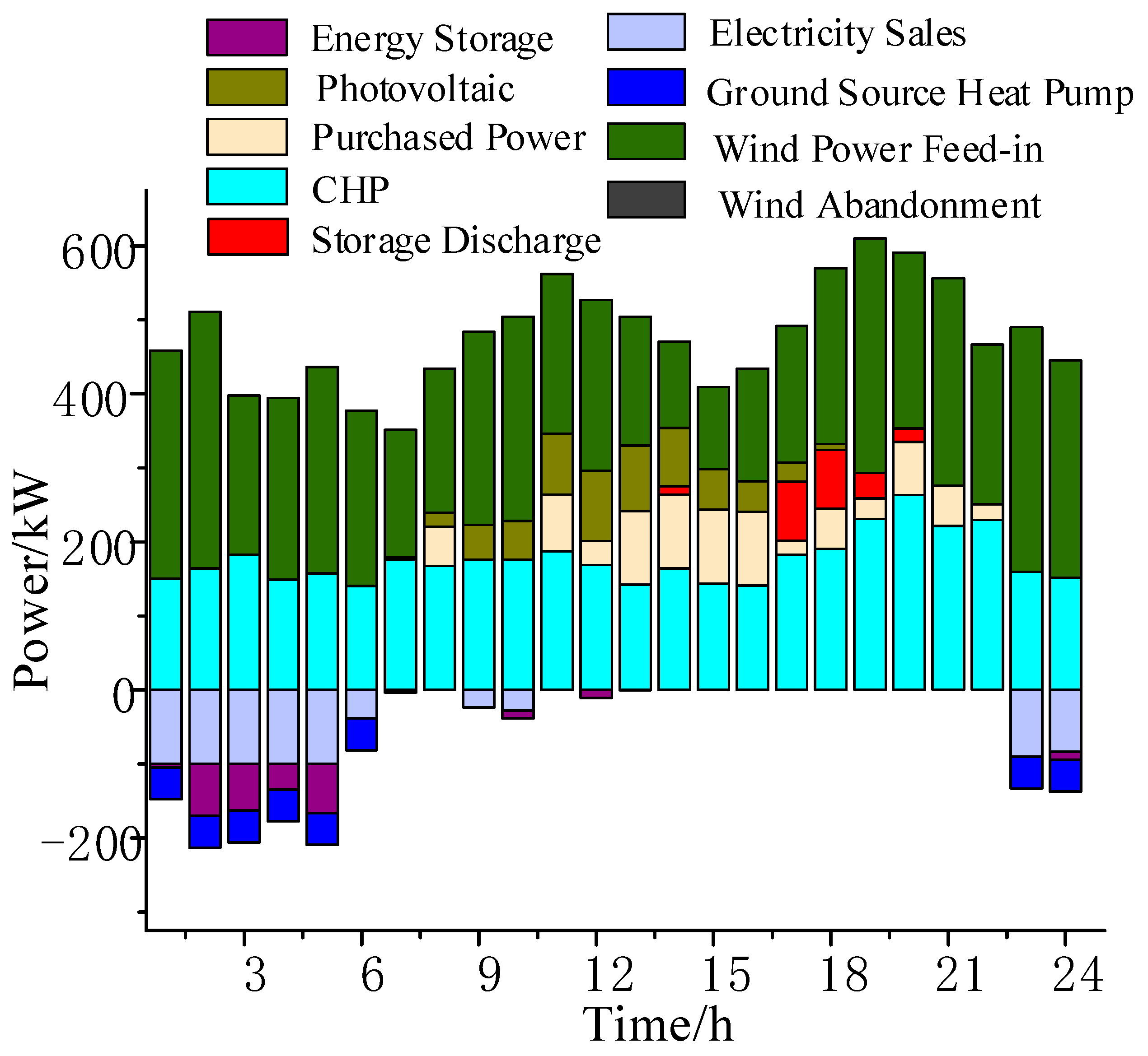
6.2. Optimized Operation Results and Analysis

The optimal scheduling results of the RIES are shown in Figure 6, Figure 7, Figure 8 and Figure 9 and Table 4: The scheduling results of Scenario 1 are shown in Figure 6; at this time, the electric load of the RIES mainly consists of electricity purchased and sold between the CHP, wind power, PV, storage battery, and the main grid. During the hours of 1:00–7:00 and 23:00–24:00, the electricity price is in the trough, so the CHP units and the ground source heat pumps are operating in the heat-to-power mode. However, limited by the transmission power of the contact line, there is wind abandonment in the system, resulting in energy waste.
Scenario 2 considers the effect of a low-temperature environment on the available capacity and energy transfer rate of the energy storage system on the basis of Scenario 1, and its scheduling results are shown in Figure 7 and Table 4. From the figure, it can be seen that the peak-to-valley difference in the system increases by 2.33% compared with Scenario 1, the abandoned wind rate increases by 4.12%, and the total cost increases by 1.53%. This is because the available capacity and the charging and discharging rate of the storage battery are affected in the low-temperature environment, and in the time period of 1:00–7:00, the actual available capacity of the electric storage is limited to be insufficient, and it is difficult to consume the wind power output in this time period, which leads to a significant increase in the phenomenon of wind abandonment. At 17:00–18:00, the purchase price of electricity gradually increases, and the battery is limited by the actual available capacity, making it difficult to provide a sufficient load to the users, which results in the purchase cost of Scenario 2 being higher than that of Scenario 1. At the same time, the heat loss increases in a low-temperature environment, and it is necessary to increase the output of bromine chillers and ground source heat pumps to maintain the heat balance, which further raises the operating cost of Scenario 2.
Scenario 3 introduces a combined heat and power demand response mechanism on the basis of Scenario 2, and its scheduling results are shown in Figure 8 and Table 4. As can be seen from the figure, the system wind power consumption rate increases by 5.95% compared with Scenario 2, the peak-to-valley difference decreases by 5.04%, and the total cost decreases by 1.04%. The distribution of electricity consumption is optimized by introducing the combined heat and power demand response mechanism to regulate the user’s electricity consumption habits. During 1:00–7:00 and 23:00–24:00, the price of electricity at the customer side is lowered to guide users to use electricity and increase the consumption of electricity in the valley; during 8:00–22:00, the price of electricity at the customer side is raised to reduce the willingness of users to use electricity, which in turn reduces the load of electricity in that period, reduces the difference between the peaks and valleys of the system, and, at the same time, promotes the consumption of wind power. In addition, the combined heat and power demand response mechanism allows for a limited adjustment of the heat load to better adapt to the time-varying electricity price. At 12:00–18:00, the purchased power price is slightly lower than the generation cost of the CHP unit, and the temperature is higher, so by appropriately lowering the indoor temperature, the CHP unit’s output is reduced, and the purchased power is increased, reducing the overall cost. At 19:00–22:00, the purchased power price is higher than the CHP unit generation cost, and the purchased power cost of the system is reduced by appropriately increasing the indoor temperature so that the CHP unit operates at full capacity, and the excess heat is stored in the heat storage tank.
Scenario 4 adds a battery insulation device on the basis of Scenario 3, which keeps the battery in the best working condition all the time by increasing part of the thermal load. The dispatch results are shown in Figure 9 and Table 4. Compared with Scenario 3, the peak-to-valley difference in the system is reduced by 10.03%, and the total cost is reduced by 2.55%. Although the thermal load of the system is increased by the input of the heater device, the increase in the effective capacity enables the electric storage to provide a large amount of electricity when the purchase price of electricity is higher than the system generation cost, from 17:00 to 19:00, effectively reducing the purchase cost of the electricity and realizing the complete consumption of wind power in the time period from 1:00 to 7:00.
The results of the optimal scheduling of heat load and the integrated cost for each scenario in this process are shown in Figure 10. Scenario 2 takes into account that the heat dissipation of the heat storage tank increases significantly in a low-temperature environment, and the heat load increases by 4.71% compared with Scenario 1 due to heat loss.
Scenario 3 introduces a heat load response mechanism to regulate the indoor temperature on the basis of Scenario 2, which reduces the demand for heat load without affecting the comfort of the residents. As can be seen from Figure 10, the heat load of Scenario 3 is higher than that of Scenario 2 in the time periods of 7:00–11:00 and 19:00–22:00, and the heat load of Scenario 2 is higher than that of Scenario 3 in the time periods of 1:00–7:00 and 12:00–18:00.This is due to the fact that the purchased price of electricity is higher than the cost of power generation of the CHP unit during the time periods 8:00–11:00 and 19:00–22:00, and the heat load of Scenario 2 is higher than Scenario 3 for the purpose of decreasing the amount of electricity purchased from the power grid. This is due to the fact that the power purchase price is higher than the power generation cost of CHP units in 8:00–11:00 and 19:00–22:00, and the room temperature is increased to reduce the power purchased from the grid, which increases the power generation of the CHP units; the power purchase price is lower than the power generation cost of the CHP units at 1:00–7:00 and 12:00–18:00, and the power purchased is increased by lowering the heat load and decreasing the power output of the CHP units. This also leads to the ineffectiveness of heat load optimization in this scenario, and the heat load only decreases by 0.54% compared to Scenario 2.
Scenario 4 increases the thermal load of the system by 0.42% compared with Scenario 3 due to the additional consumption of thermal load by the additional storage heater, but it effectively improves the comprehensive benefit of the system by realizing the complete consumption of wind power.

6.3. Analysis of the Effect of Weighting Coefficients on the Results of RIES Scheduling

The weighting coefficient can reflect the degree of risk preference of the decision maker [35]; in order to explore the influence of the weighting coefficient β on the scheduling results of the RIES, the paper derives the scheduling results under different weighting coefficients under Scenario 4 according to the change of weighting coefficients from 0.1 to 0.9, as shown in Figure 11. The results show that in the process of gradually increasing weight coefficients, the total system cost gradually increases, the expected cost share gradually increases, and the CVaR share gradually decreases. This indicates that the greater the degree of risk preference of the decision maker, the smaller the CVaR percentage While it can be effective in improving the operational safety of the system, it can also reduce the economy of the system. In actual scheduling, operators should choose appropriate weighting coefficients to balance the benefits and risks of the system according to specific needs.

7. Conclusions

By establishing a coordinated and optimized operation model of a RIES considering wind power consumption in a low-temperature environment, the following conclusions can be drawn based on the comparative analysis of the four scenarios:
(1)
The fine energy storage model takes into account the influence of ambient temperature, capacity, and other constraints, the equipment output is more in line with the actual situation than the traditional energy storage model, and the reliability of the system optimization and scheduling is higher.
(2)
Comprehensive consideration of electricity and heat flexible load demand response can effectively reduce the peak and valley difference in the user load while taking into account the wind power consumption capacity and economic benefits.
(3)
Compared to traditional deterministic models, it is more reasonable to utilize the CVaR theory to describe the risk of returns from wind power uncertainty.
(4)
The adjustment of the weight coefficients in the CVaR theory according to the historical operation information and the actual situation during the actual scheduling process can further improve the comprehensive efficiency of the system.

Author Contributions

Conceptualization, L.L. and J.H.; methodology, L.L.; software, L.L.; validation, J.H. and Z.L.; formal analysis, L.L.; investigation, H.Q.; resources, H.Q.; data curation, H.Q.; writing—original draft preparation, L.L.; writing—review and editing, L.L.; visualization, L.L.; supervision, J.H.; project administration, Z.L.; funding acquisition, Z.L. All authors have read and agreed to the published version of the manuscript.

Funding

This work was supported by the National Natural Science Foundation of China, grant number 52077120. Project Manager is Zhenxing Li.

Data Availability Statement

Data are contained within the article.

Acknowledgments

The authors thank the hard work of all the anonymous reviewers for improving the quality of this submission.

Conflicts of Interest

The authors declare no conflict of interest.

Abbreviations

The following abbreviations are used in this manuscript:
RIESRegional Integrated Energy Systems
CvaRConditional Value-at-Risk
CHPCombined, Heating and Power
IDRIntegrated Demand Response
IESIntegrated Energy Storage
WTWind Turbines
PVPhotovoltaic
GSHPGround Source Heat Pumps
HSTHeat Storage Tank
BCBromine Chiller
GTGas Turbine
PBDRPrice-Based Demand Response
PMVPredicted Mean Vote
VaRValue at Risk
O&MOperation and Maintenance

References

  1. Wang, Y.; Wang, Y.; Huang, Y.; Li, F.; Zeng, M.; Li, J.; Wang, X.; Zhang, F. Planning and operation method of the regional integrated energy system considering economy and environment. Energy 2019, 171, 731–750. [Google Scholar] [CrossRef]
  2. Wang, Y.; Lu, Y.; Ju, L.; Wang, T.; Tan, Q.; Wang, J.; Tan, Z. A multi-objective scheduling optimization model for hybrid energy system connected with wind-photovoltaic-conventional gas turbines, CHP considering heating storage mechanism. Energies 2019, 12, 425. [Google Scholar] [CrossRef]
  3. Wang, J.; Deng, H.; Qi, X. Cost-based site and capacity optimization of multi-energy storage system in the regional integrated energy networks. Energy 2022, 261, 125240. [Google Scholar] [CrossRef]
  4. Xu, J.; Wang, X.; Gu, Y.; Ma, S. A data-based day-ahead scheduling optimization approach for regional integrated energy systems with varying operating conditions. Energy 2023, 283, 128534. [Google Scholar] [CrossRef]
  5. Guo, Z.; Zhang, R.; Wang, L.; Zeng, S.; Li, Y. Optimal operation of regional integrated energy system considering demand response. Appl. Therm. Eng. 2021, 191, 116860. [Google Scholar] [CrossRef]
  6. Zhang, S.; Miao, S.; Li, Y.; Yin, B.; Li, C. Regional integrated energy system dispatch strategy considering advanced adiabatic compressed air energy storage device. Int. J. Electr. Power Energy Syst. 2021, 125, 106519. [Google Scholar] [CrossRef]
  7. Zhu, H.; Li, H.; Liu, G.; Ge, Y.; Shi, J.; Li, H.; Zhang, N. Energy storage in high renewable penetration power systems: Technologies, applications, supporting policies and suggestions. CSEE J. Power Energy Syst. 2020, 1–9. [Google Scholar] [CrossRef]
  8. Zheng, W.; Lu, H.; Zhang, M.; Wu, Q.; Hou, Y.; Zhu, J. Distributed energy management of multi-entity integrated electricity and heat systems: A review of architectures, optimization algorithms, and prospects. IEEE Trans. Smart Grid 2023. [Google Scholar] [CrossRef]
  9. Zhang, Y.; Huang, Z.; Zheng, F.; Zhou, R.; Le, J.; An, X. Cooperative optimization scheduling of the electricity-gas coupled system considering wind power uncertainty via a decomposition-coordination framework. Energy 2020, 194, 116827. [Google Scholar] [CrossRef]
  10. Sun, G.; Li, Y.; Chen, S.; Wei, Z.; Chen, S.; Zang, H. Dynamic stochastic optimal power flow of wind power and the electric vehicle integrated power system considering temporal-spatial characteristics. J. Renew. Sustain. Energy 2016, 8, 053309. [Google Scholar] [CrossRef]
  11. Ju, L.; Li, H.; Zhao, J.; Chen, K.; Tan, Q.; Tan, Z. Multi-objective stochastic scheduling optimization model for connecting a virtual power plant to wind-photovoltaic-electric vehicles considering uncertainties and demand response. Energy Convers. Manag. 2016, 128, 160–177. [Google Scholar] [CrossRef]
  12. Li, P.; Yu, D.; Yang, M.; Wang, J. Flexible look-ahead dispatch realized by robust optimization considering CVaR of wind power. IEEE Trans. Power Syst. 2018, 33, 5330–5340. [Google Scholar] [CrossRef]
  13. Levy, D.; Carmon, Y.; Duchi, J.C.; Sidford, A. Large-scale methods for distributionally robust optimization. Adv. Neural Inf. Process. Syst. 2020, 33, 8847–8860. [Google Scholar]
  14. Wang, Y.; Li, F.; Yang, J.; Zhou, M.; Song, F.; Zhang, D.; Xue, L.; Zhu, J. Demand response evaluation of RIES based on improved matter-element extension model. Energy 2020, 212, 118121. [Google Scholar] [CrossRef]
  15. Zhao, D.; Xia, X.; Tao, R. Optimal configuration of electric-gas-thermal multi-energy storage system for regional integrated energy system. Energies 2019, 12, 2586. [Google Scholar] [CrossRef]
  16. Yang, L.; Han, Q.; Li, X. Economic Dispatch of Multi Region Electric and Heat Energy System Using Two Stage Demand Response for Better Integration of Wind Power. J. Electr. Eng. Technol. 2022, 17, 2553–2563. [Google Scholar] [CrossRef]
  17. Wang, J.; Zong, Y.; You, S.; Træholt, C. A review of Danish integrated multi-energy system flexibility options for high wind power penetration. Clean Energy 2017, 1, 23–35. [Google Scholar] [CrossRef]
  18. Zhang, Q.; Zhang, L.; Nie, J.; Li, Y. Techno-economic analysis of air source heat pump applied for space heating in northern China. Appl. Energy 2017, 207, 533–542. [Google Scholar] [CrossRef]
  19. Cai, B.; Li, H.; Hu, Y.; Liu, L.; Huang, J.; Lazzaretto, A.; Zhang, G. Theoretical and experimental study of combined heat and power (CHP) system integrated with ground source heat pump (GSHP). Appl. Therm. Eng. 2017, 127, 16–27. [Google Scholar] [CrossRef]
  20. Matjanov, E. Gas turbine efficiency enhancement using absorption chiller. Case study for Tashkent CHP. Energy 2020, 192, 116625. [Google Scholar] [CrossRef]
  21. Fatullah, M.A.; Rahardjo, A.; Husnayain, F. Analysis of discharge rate and ambient temperature effects on lead acid battery capacity. In Proceedings of the 2019 IEEE International Conference on Innovative Research and Development (ICIRD), Jakarta, Indonesia, 28–30 June 2019; pp. 1–5. [Google Scholar]
  22. Low, W.Y.; Abdul Aziz, M.J.; Idris, N.R.N. Modelling of lithium-titanate battery with ambient temperature effect for charger design. IET Power Electron. 2016, 9, 1204–1212. [Google Scholar] [CrossRef]
  23. Ruetschi, P. Aging mechanisms and service life of lead–acid batteries. J. Power Sources 2004, 127, 33–44. [Google Scholar] [CrossRef]
  24. Arslan, M.; Igci, A.A. Thermal performance of a vertical solar hot water storage tank with a mantle heat exchanger depending on the discharging operation parameters. Sol. Energy 2015, 116, 184–204. [Google Scholar] [CrossRef]
  25. Cabeza, L.F. Advances in thermal energy storage systems: Methods and applications. In Advances in Thermal Energy Storage Systems; Elsevier: Amsterdam, The Netherlands, 2021; pp. 37–54. [Google Scholar]
  26. Yang, C.; Meng, C.; Zhou, K. Residential electricity pricing in China: The context of price-based demand response. Renew. Sustain. Energy Rev. 2018, 81, 2870–2878. [Google Scholar] [CrossRef]
  27. Shewale, A.; Mokhade, A.; Funde, N.; Bokde, N.D. An overview of demand response in smart grid and optimization techniques for efficient residential appliance scheduling problem. Energies 2020, 13, 4266. [Google Scholar] [CrossRef]
  28. Wang, Y.; Huang, Y.; Wang, Y.; Zeng, M.; Yu, H.; Li, F.; Zhang, F. Optimal scheduling of the RIES considering time-based demand response programs with energy price. Energy 2018, 164, 773–793. [Google Scholar] [CrossRef]
  29. Yau, Y.; Chew, B. A review on predicted mean vote and adaptive thermal comfort models. Build. Serv. Eng. Res. Technol. 2014, 35, 23–35. [Google Scholar] [CrossRef]
  30. Gao, B.; Pan, Y.; Chen, Z.; Wu, F.; Ren, X.; Hu, M. A spatial conditioned Latin hypercube sampling method for mapping using ancillary data. Trans. GIS 2016, 20, 735–754. [Google Scholar] [CrossRef]
  31. Stoyanov, S.V.; Rachev, S.T.; Fabozzi, F.J. Sensitivity of portfolio VaR and CVaR to portfolio return characteristics. Ann. Oper. Res. 2013, 205, 169–187. [Google Scholar] [CrossRef]
  32. Rockafellar, R.T.; Uryasev, S. Optimization of conditional value-at-risk. J. Risk 2000, 2, 21–42. [Google Scholar] [CrossRef]
  33. Dong, L.; Li, M.; Hu, J.; Chen, S.; Zhang, T.; Wang, X.; Pu, T. A hierarchical game approach for optimization of regional integrated energy system clusters considering bounded rationality. CSEE J. Power Energy Syst. 2023, 1–11. [Google Scholar] [CrossRef]
  34. Li, P.; Yang, M.; Wu, Q. Confidence interval based distributionally robust real-time economic dispatch approach considering wind power accommodation risk. IEEE Trans. Sustain. Energy 2020, 12, 58–69. [Google Scholar] [CrossRef]
  35. Ju, L.; Tan, Q.; Lu, Y.; Tan, Z.; Zhang, Y.; Tan, Q. A CVaR-robust-based multi-objective optimization model and three-stage solution algorithm for a virtual power plant considering uncertainties and carbon emission allowances. Int. J. Electr. Power Energy Syst. 2019, 107, 628–643. [Google Scholar] [CrossRef]
Figure 1. Basic structure of the RIES.
Energies 16 07791 g001
Figure 2. Predictive output of wind, photovoltaic, and electrical heating loads.
Energies 16 07791 g002
Figure 3. Temperature and purchase-sale price.
Energies 16 07791 g003
Figure 4. Wind power sample space.
Energies 16 07791 g004
Figure 5. Wind power landscape reduction.
Energies 16 07791 g005
Figure 6. Scenario 1 scheduling results.
Energies 16 07791 g006
Figure 7. Scenario 2 scheduling results.
Energies 16 07791 g007
Figure 8. Scenario 3 scheduling result.
Energies 16 07791 g008
Figure 9. Scenario 4 scheduling result.
Energies 16 07791 g009
Figure 10. Heat load scheduling results for four scenarios.
Energies 16 07791 g010
Figure 11. Expected cost and CVaR under different weighting coefficients.
Energies 16 07791 g011
Table 1. Parameters of energy storage device.
ParameterBatteriesHeat Storage TanksParameterHeat Storage TanksBatteries
Capacity/(kW·h)200300Initial energy storage state0.20.2
Charging and discharging rate0.90.88Maximum energy storage state0.90.9
Attrition rate0.0010.01Minimum energy storage state00.2
O&M unit price (USD/kW·h)0.0510.045Maximum charge and discharge power/kW5050
Table 2. Pollutant discharge and treatment costs.
TypeSO2NOXCO2
Gas turbine emission standard (g/kWh)0.0234.795170.16
Emission standard of purchased power (g/kWh)6.42.32696
Treatment cost of each pollutant (USD/t)100019509.75
Table 3. Unit operation parameters.
ParameterGTGSHPPWPVGrid
Power upper limit/kW50030400100100
Lower power limit/kW500000
Climbing rate upper limit/(kW/min)64
Climbing rate lower limit/(kW/min)53
Efficiency0.243
O&M unit price (USD/kW·h)0.0530.0260.0290.025
Table 4. Four scenarios scheduling results.
Cost Category (USD/Day)Scenario 1Scenario 2Scenario 3Scenario 4
Total Cost5620.55706.25646.75502.5
Expected Cost5558.85648.55548.35442.4
CVaR6175.86234.46208.26043.5
Fuel Cost4292.34319.342754266.9
Maintenance Cost446.7441.1443.7455.3
Environmental Costs56.5758.6756.6454.41
Purchase and Sale Costs766.5833.8812.5665.8
Wind Abandonment Cost3.966.353.150
Wind Power Consumption Rate95.54%91.42%97.37%100%
Disclaimer/Publisher’s Note: The statements, opinions and data contained in all publications are solely those of the individual author(s) and contributor(s) and not of MDPI and/or the editor(s). MDPI and/or the editor(s) disclaim responsibility for any injury to people or property resulting from any ideas, methods, instructions or products referred to in the content.

