
Joint Multi-Objective Allocation of Parking Lots and DERs in Active Distribution Network Considering Demand Response Programs

Abstract
:1. Introduction
2. Modeling Formulation
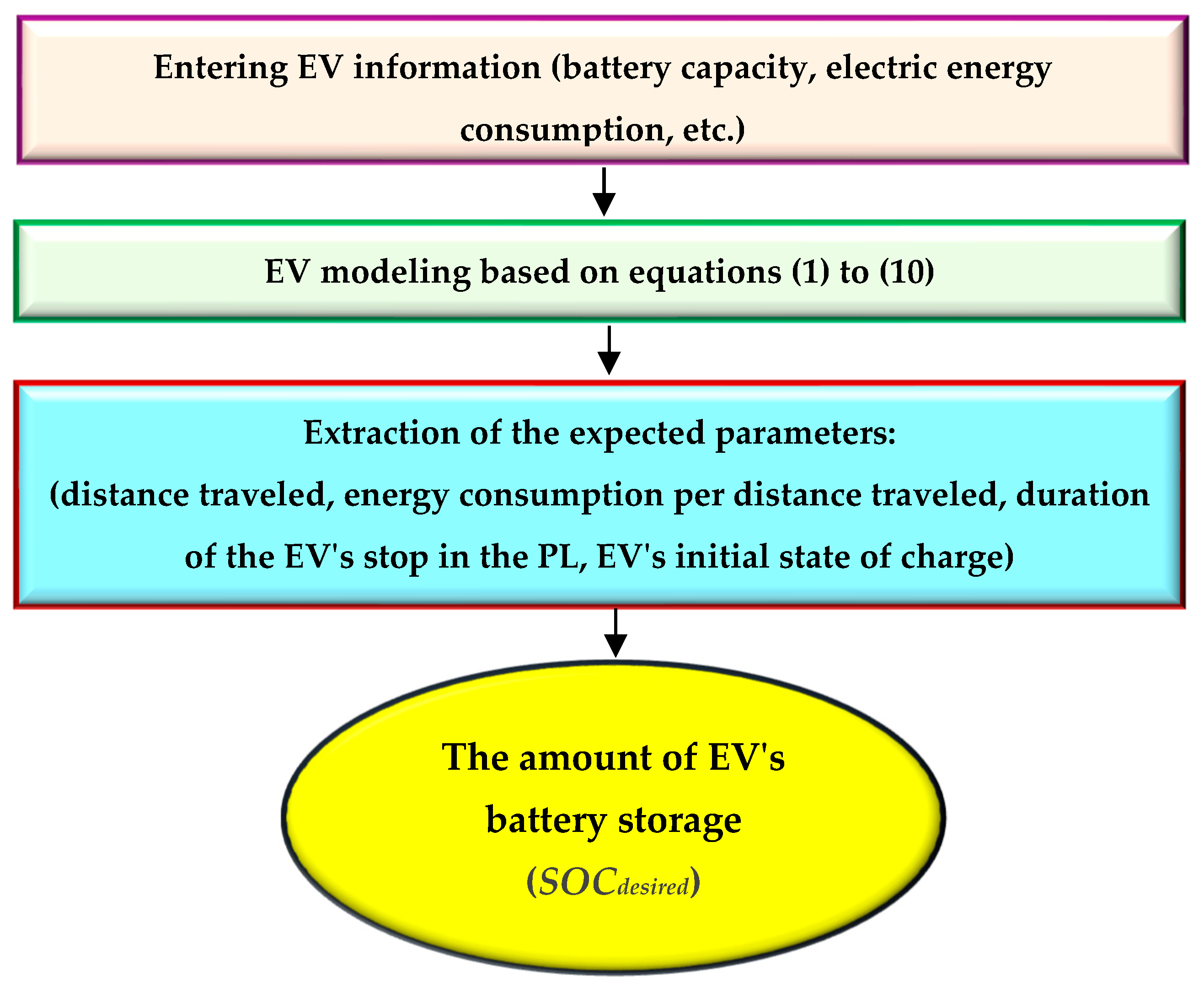
2.1. EV Modeling
2.1.1. EVs’ Expected Mileage
2.1.2. EVs’ Energy Consumption
2.1.3. Expected Availability Time of EVs in the PL
2.1.4. Initial SOC of EVs
2.2. PL Modeling
2.2.1. The Predicted Percentage of EVs in the PL at Different Hours
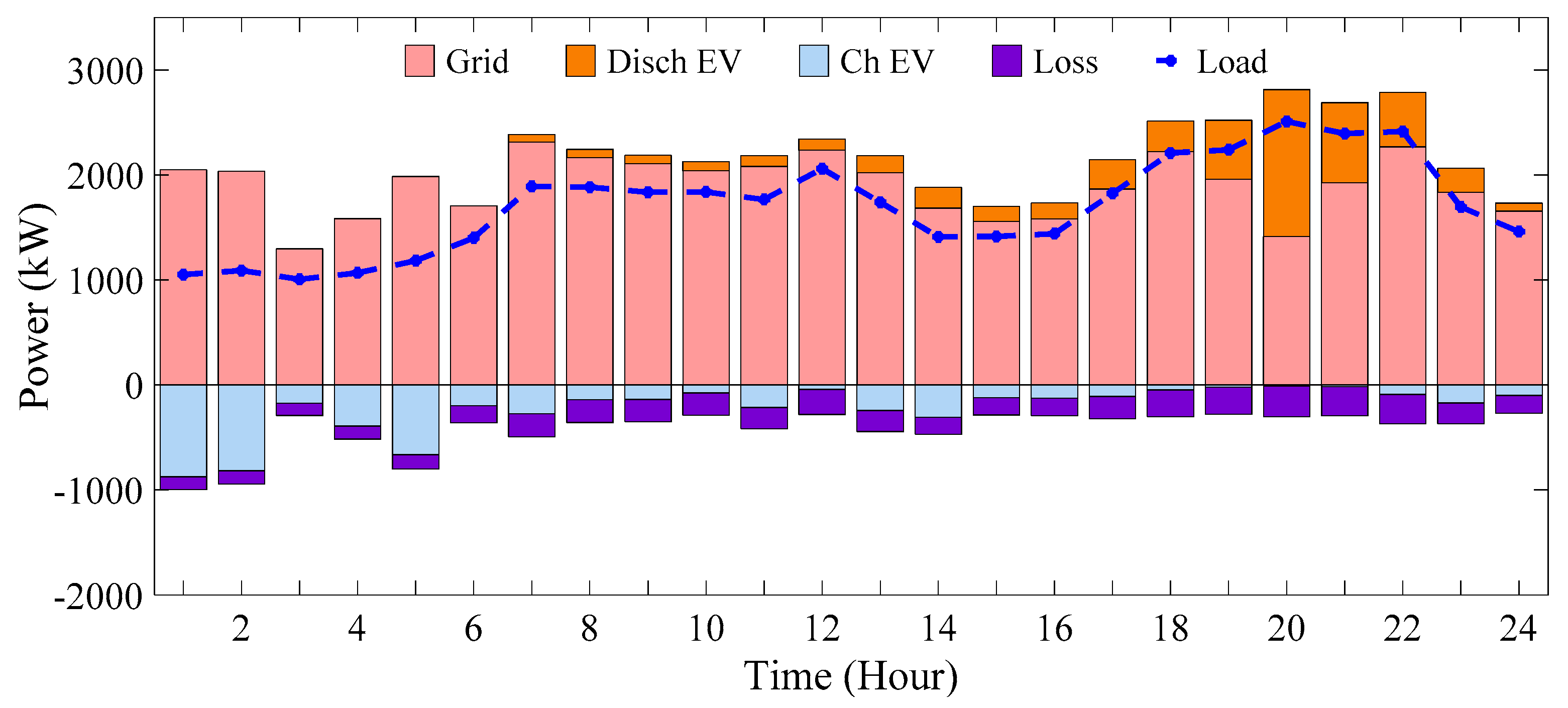
2.2.2. The Consumption/Generation Power of the PL
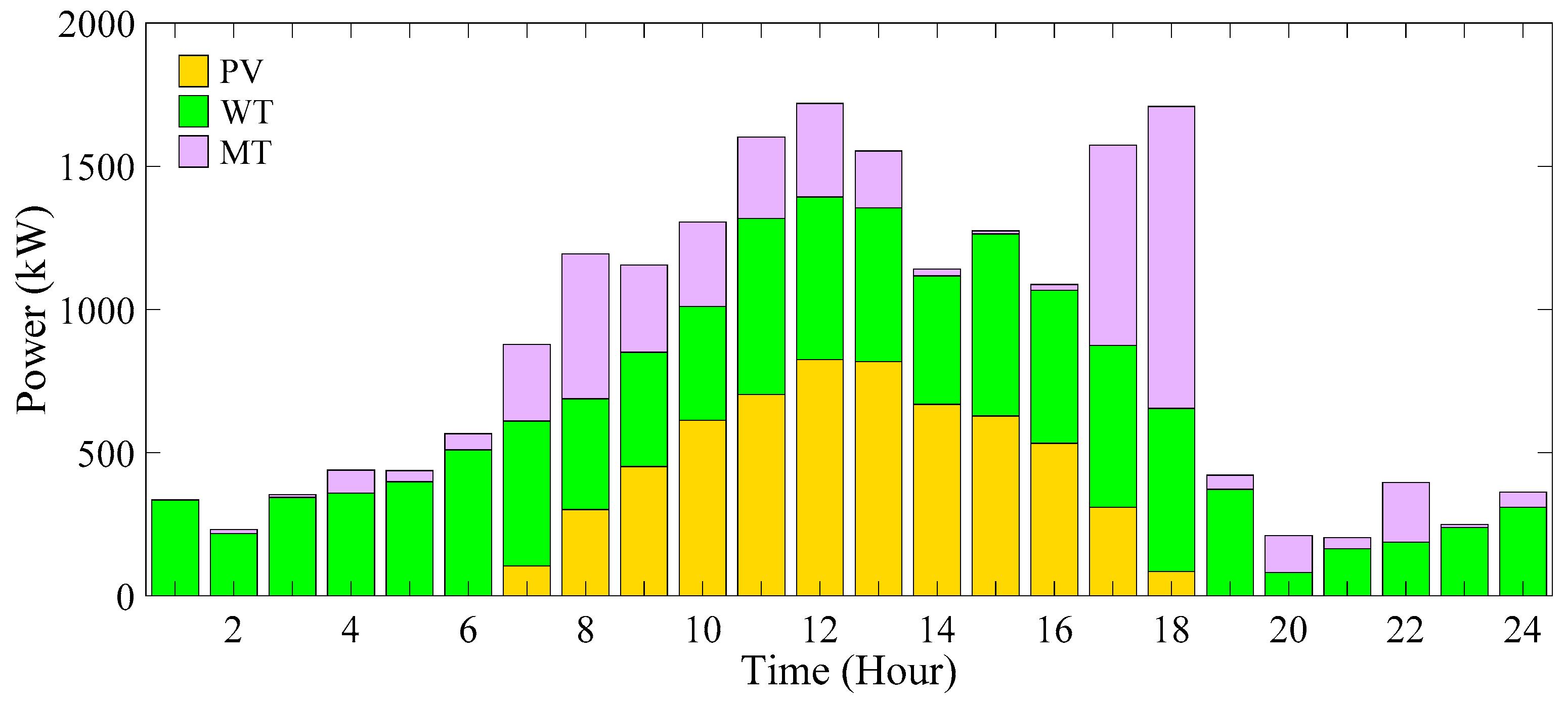
2.3. Modeling Distributed Generations
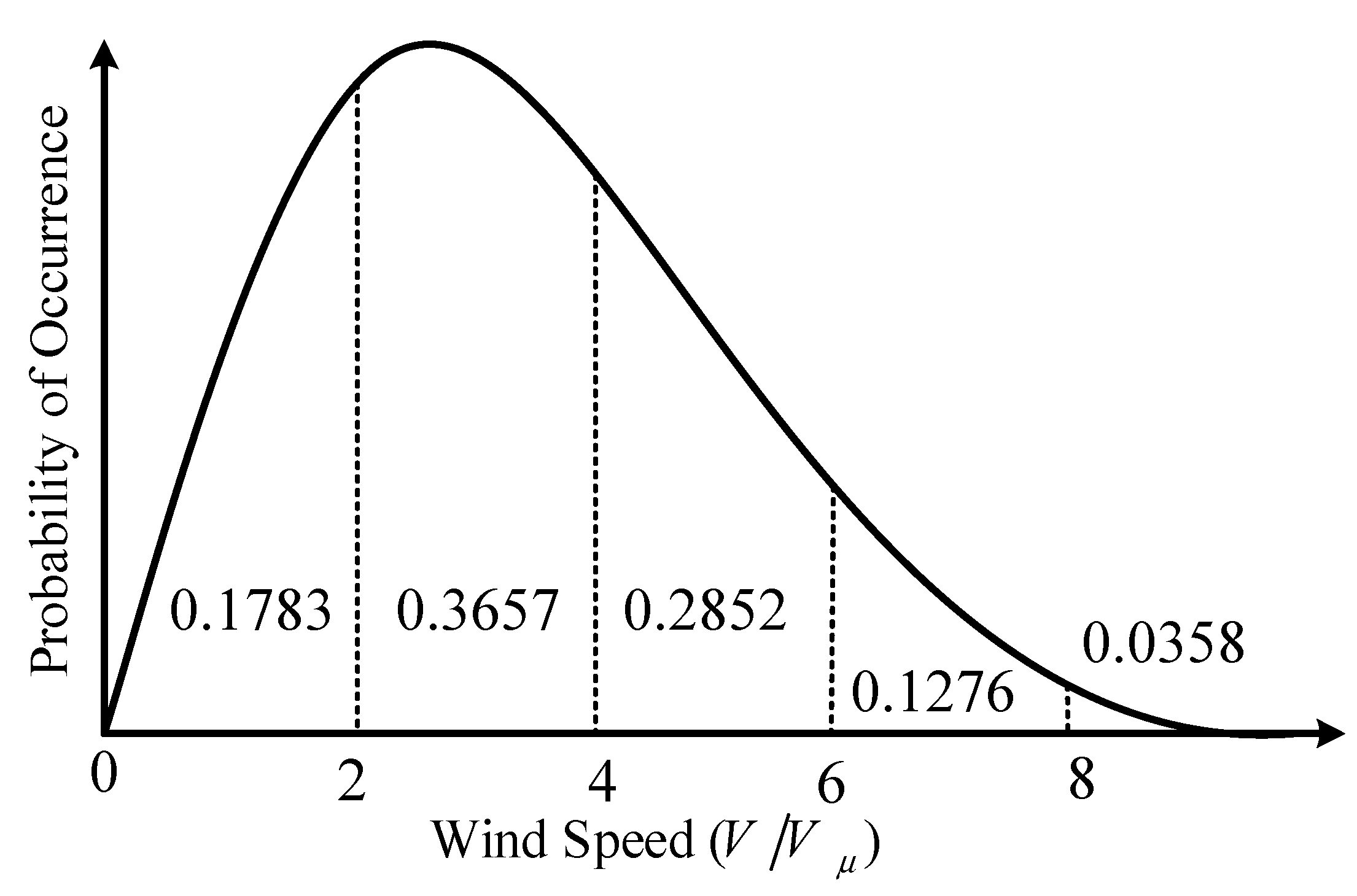
2.3.1. Wind Turbine and Wind Speed Uncertainty Modeling
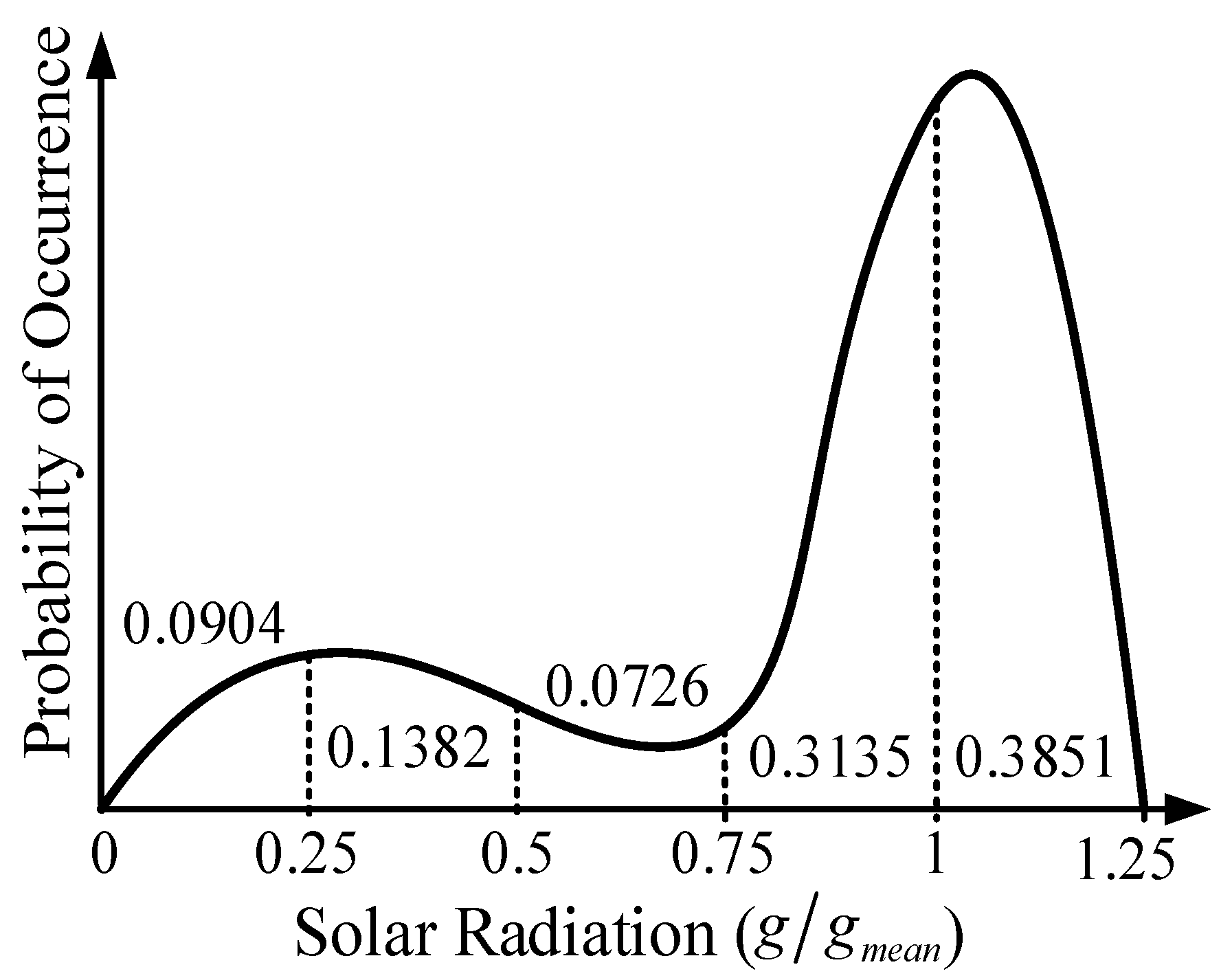
2.3.2. Solar Cell and Solar Radiation Uncertainty Modeling
2.3.3. Microturbines
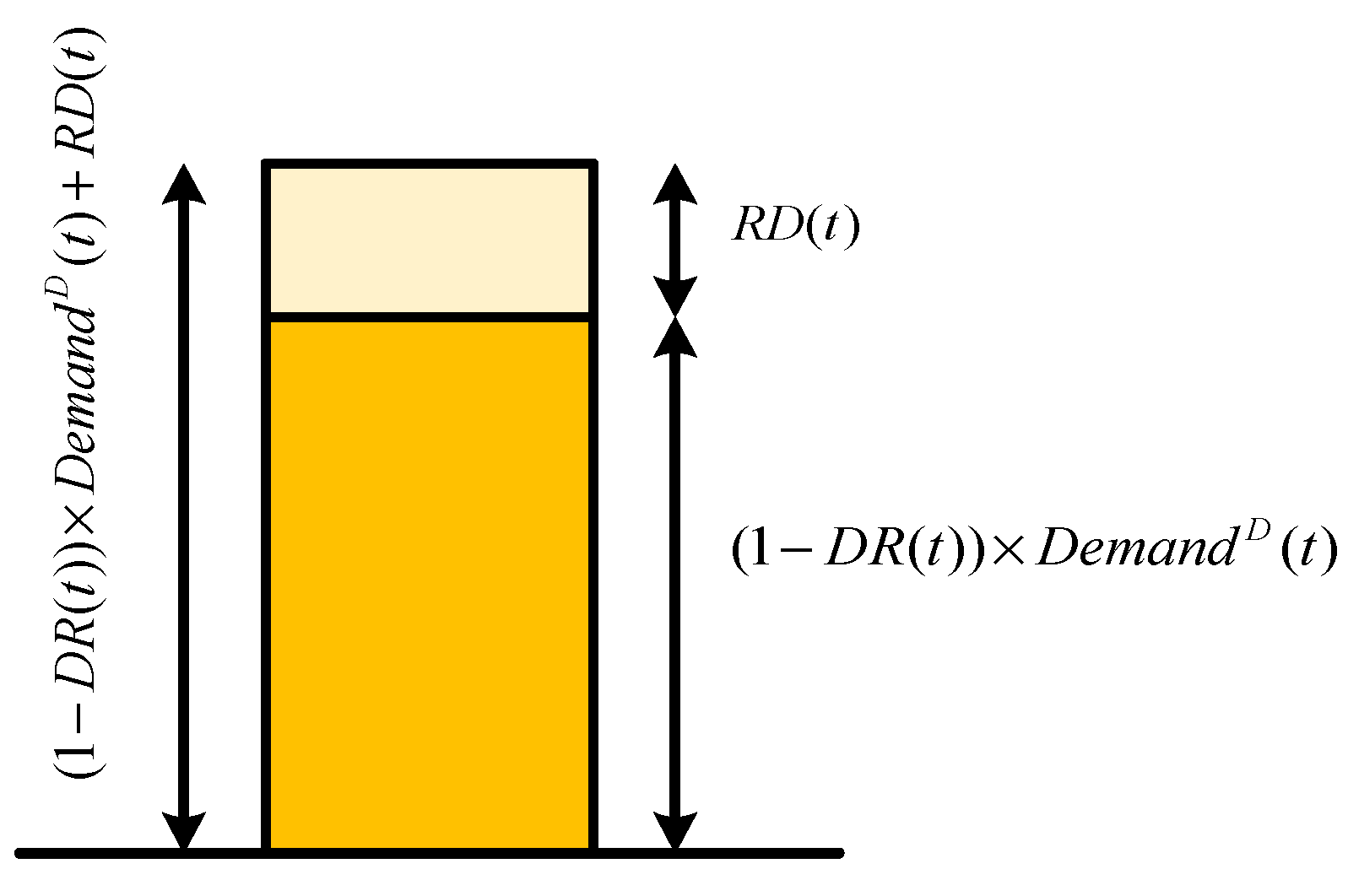
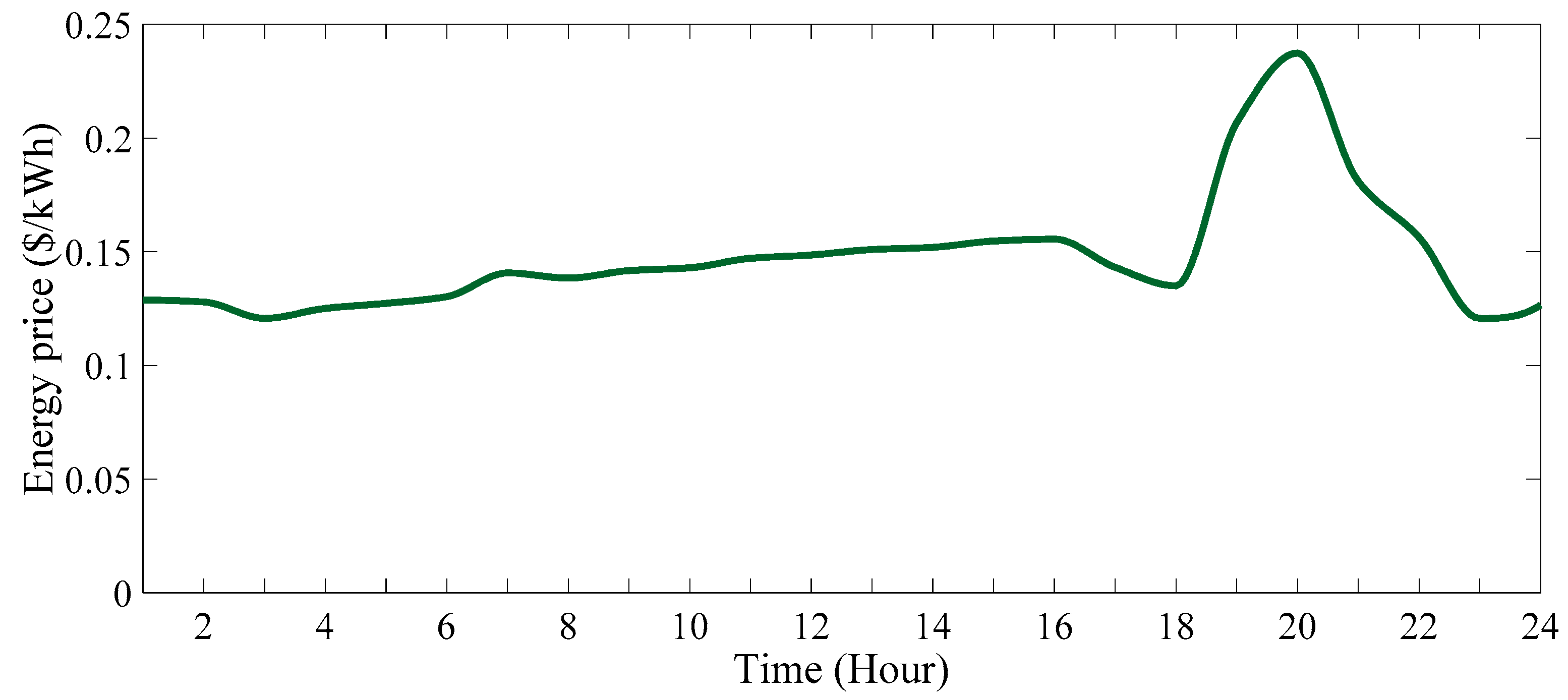
2.4. DRP Modeling
3. Problem Formulation
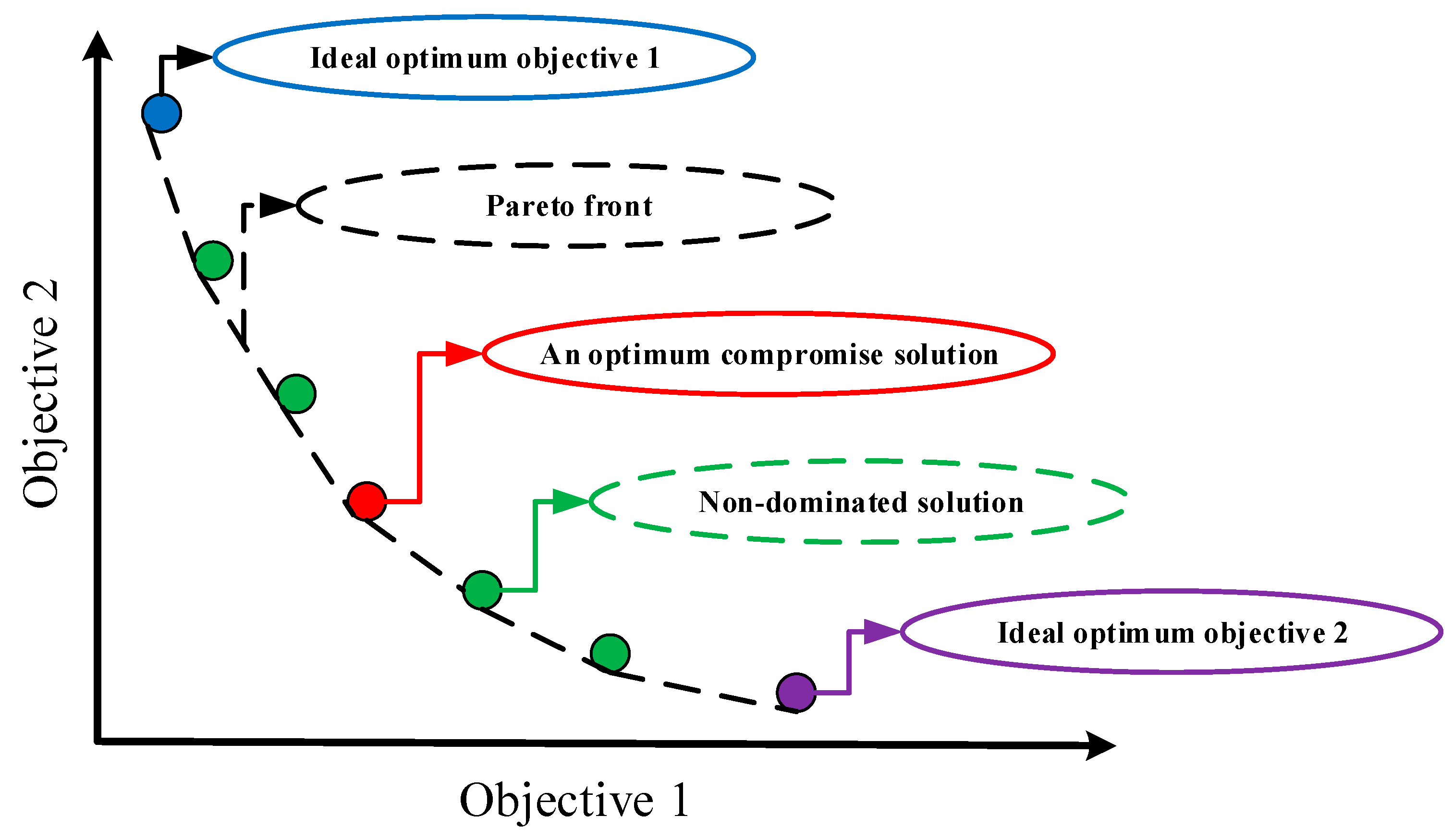
3.1. Objective Function
3.1.1. Technical Objective
- Energy Loss (f1)
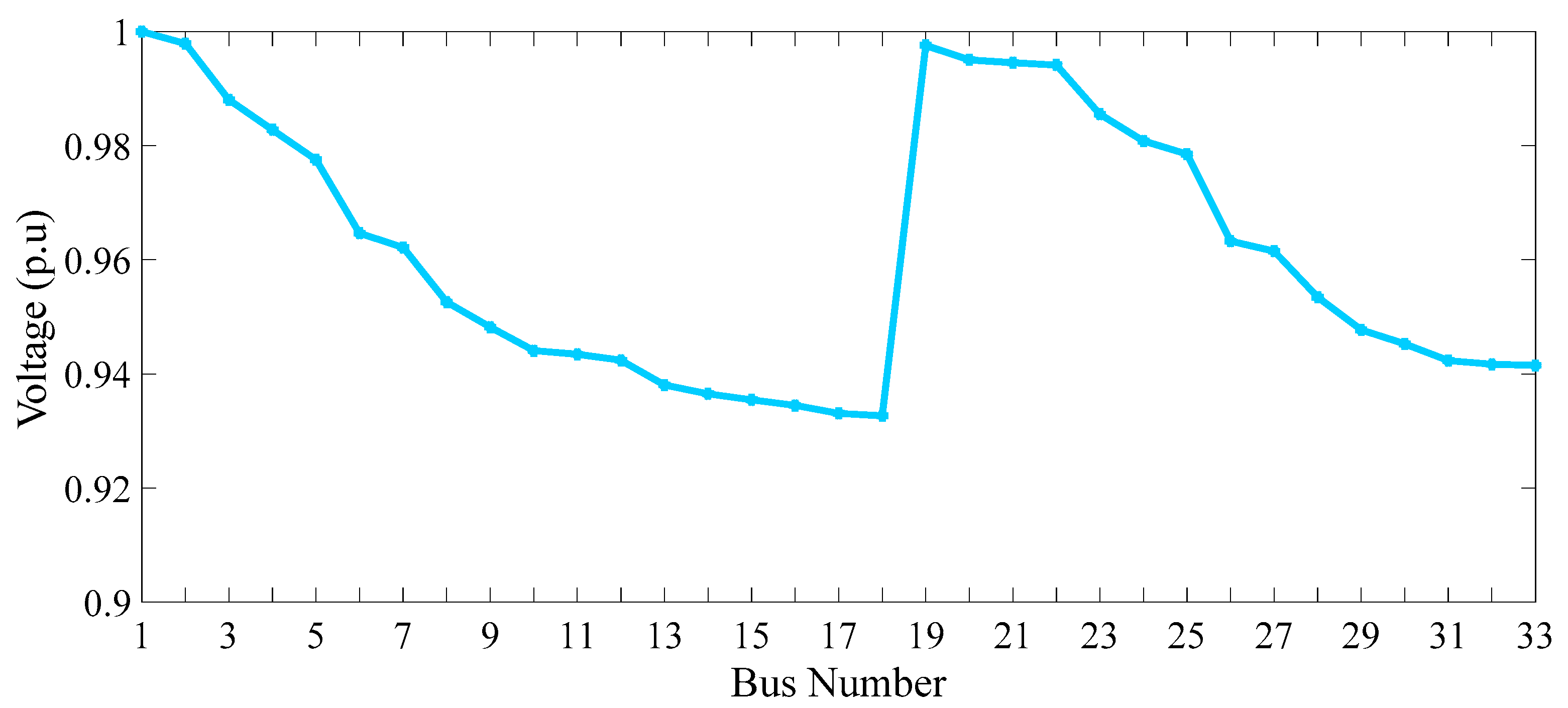
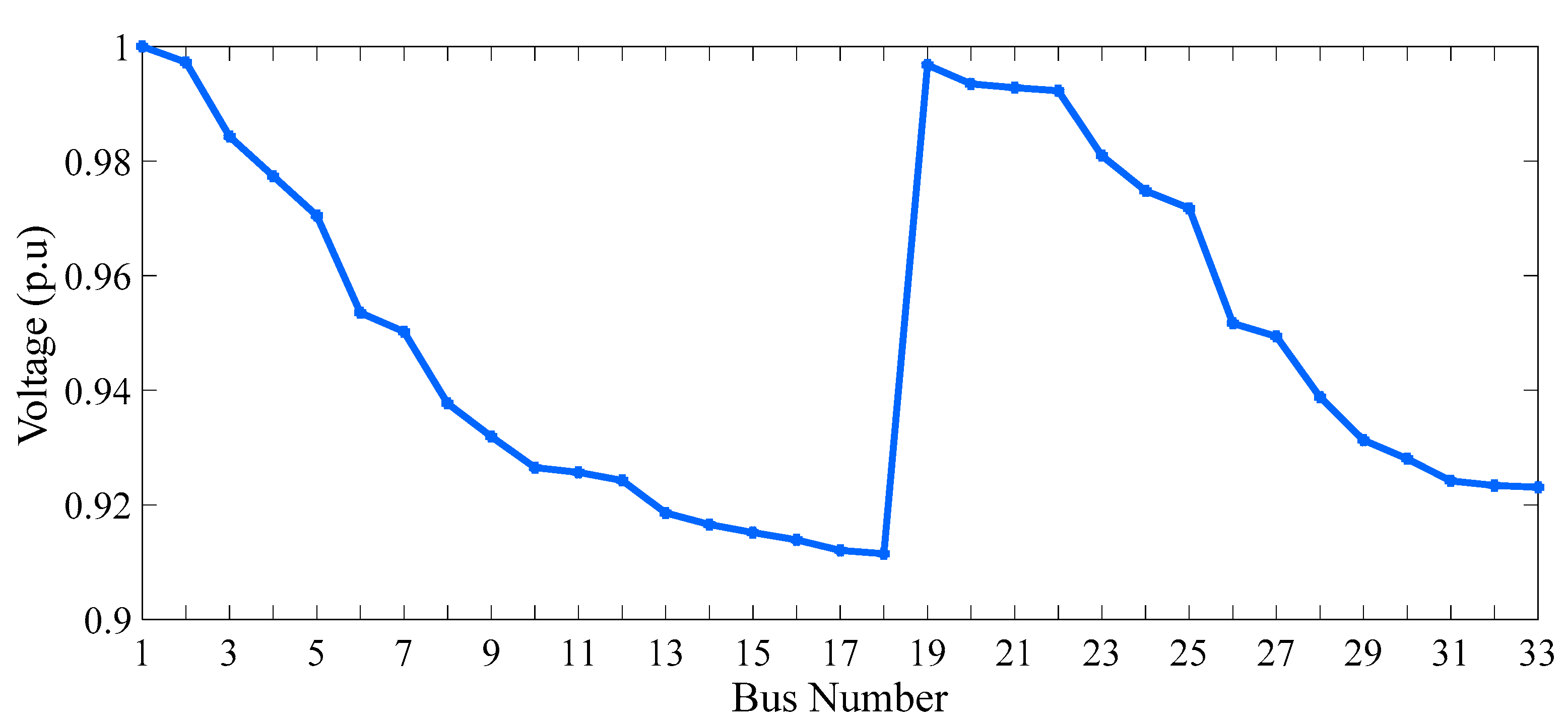
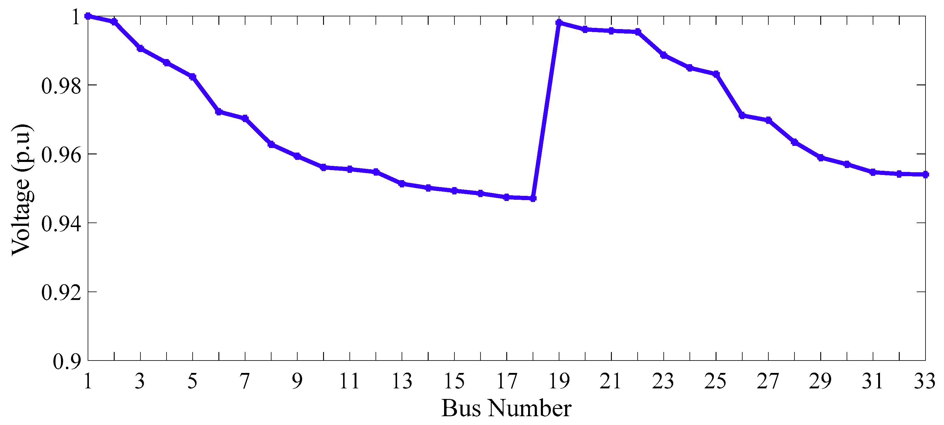
- Voltage Profile (f2)
3.1.2. Economic Objective
- The Cost of Providing Energy by DGs (f1)
- The Cost of Energy Transported from the Upstream Network (f2)
- Energy Trading Cost from/to the EVs in PLs (f3)
- The Cost of Greenhouse Gas Emissions (f4)
3.2. Constraints
3.2.1. Network Equality and Inequality Constraints
- ▪
- Power balance constraint
3.2.2. System Security Constraints
- ▪
- Distribution line capacity limit
- ▪
- Voltage drop limit
3.2.3. EVPL Constraints
- ▪
- Maximum EV charging and discharging power
- ▪
- Non-simultaneity of EV charging and discharging
- ▪
- The limit of energy stored in the EV battery
- ▪
- Parking lot capacity constraint
3.2.4. DG Constraints
- ▪
- Generation power capacity constraint
4. Problem-Solving Method
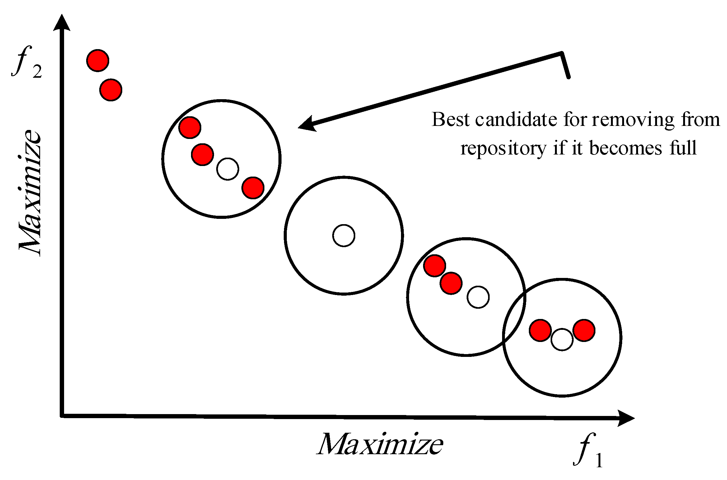
4.1. Salp Swarm Optimization Algorithm
Multi-Objective Salp Swarm Algorithm
- The SSA has the ability to store multiple solutions as the best choices for multi-objective problems.
- The SSA updates the food source with the most exceptional solution so far obtained in each iteration, and for multi-objective optimization problems, there is only one best solution.
4.2. Fuzzy Method
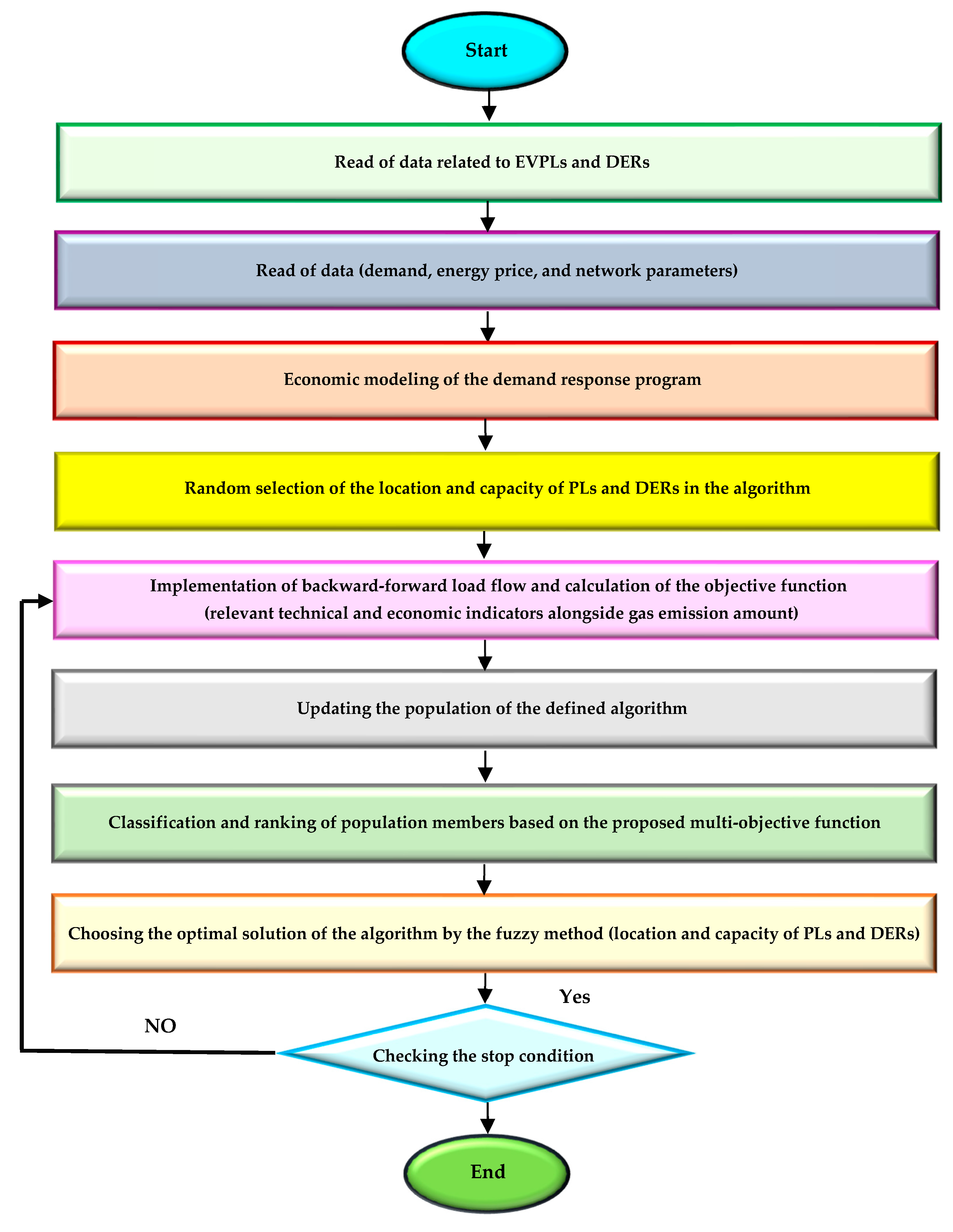
5. The Process of Implementing the Proposed Plan
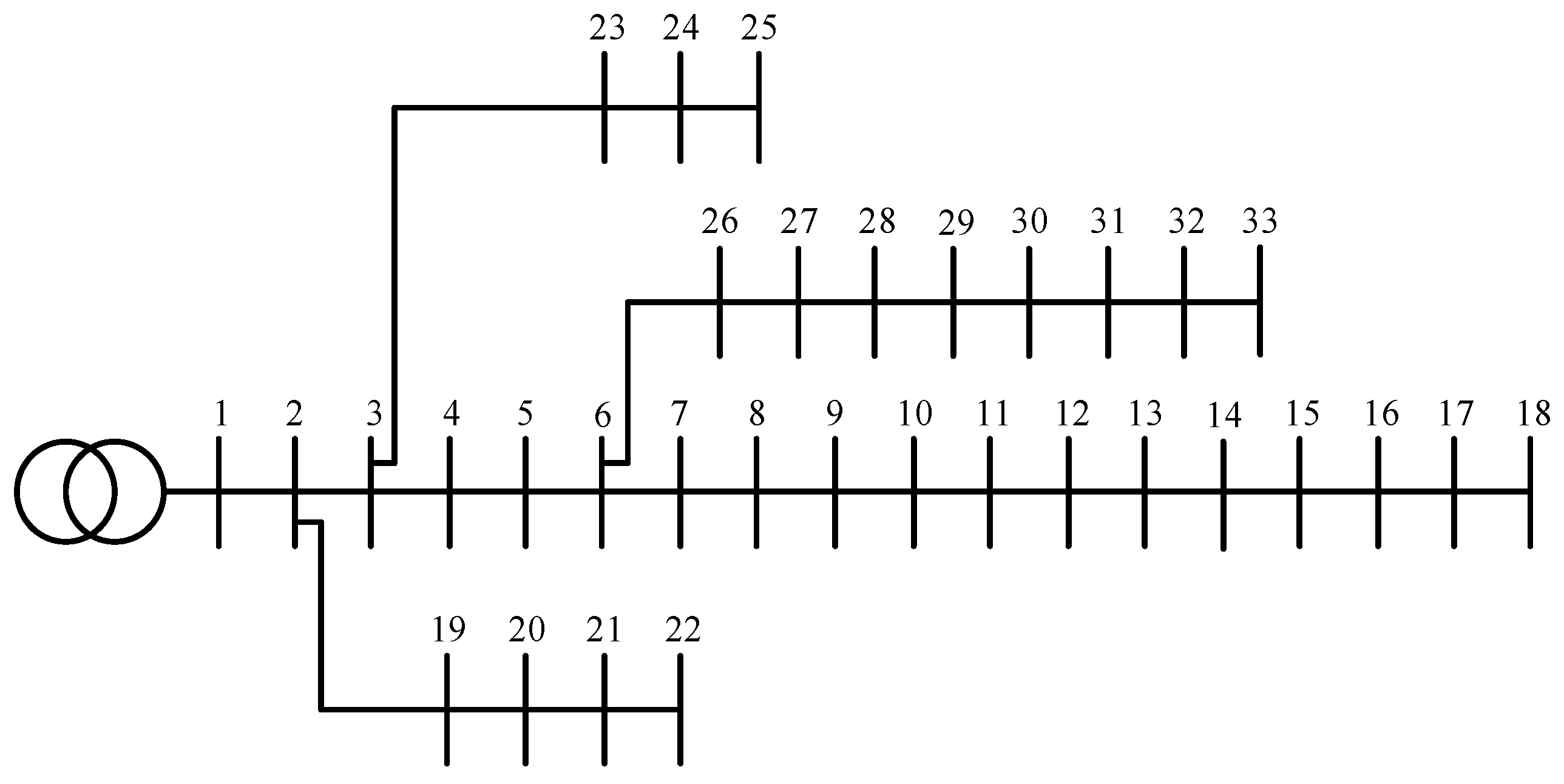
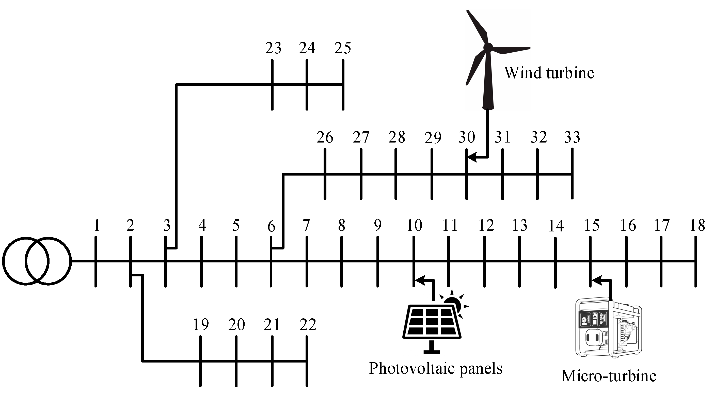
6. Case Study
- Scenario 1: Supplying the total consumption power of the distribution network by the upstream network.
- Scenario 2: Allocation of DG resources and coordinated exploitation of DG units and the network.
- Scenario 3: Allocation of PLs and their operation alongside the network (without DGs).
- Scenario 4: Coordinated exploitation of DERs, PLs, and the network to optimize the multi-objective function (without considering the DRP).
- Scenario 5: Coordinated operation of DERs, PLs, and the network to minimize the multi-objective function (taking into account the DRP).
7. Simulation Results
7.1. Results of Scenario 1
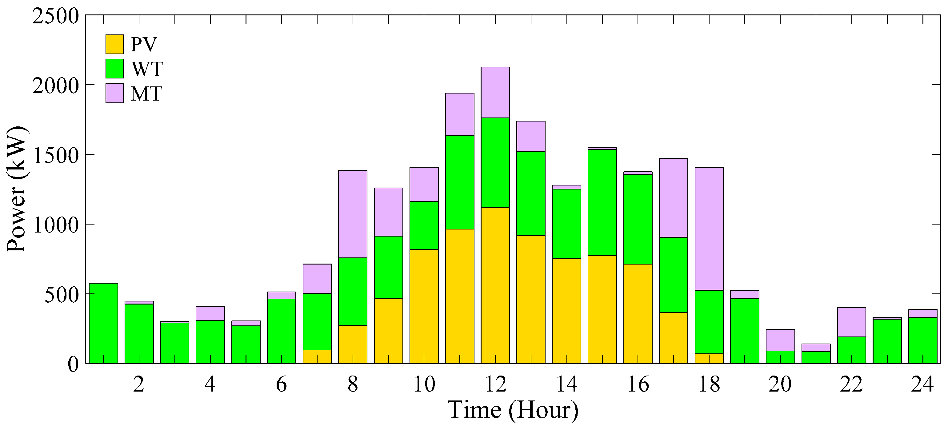
7.2. Results of Scenario 2
7.3. Results of Scenario 3
7.4. Results of Scenario 4
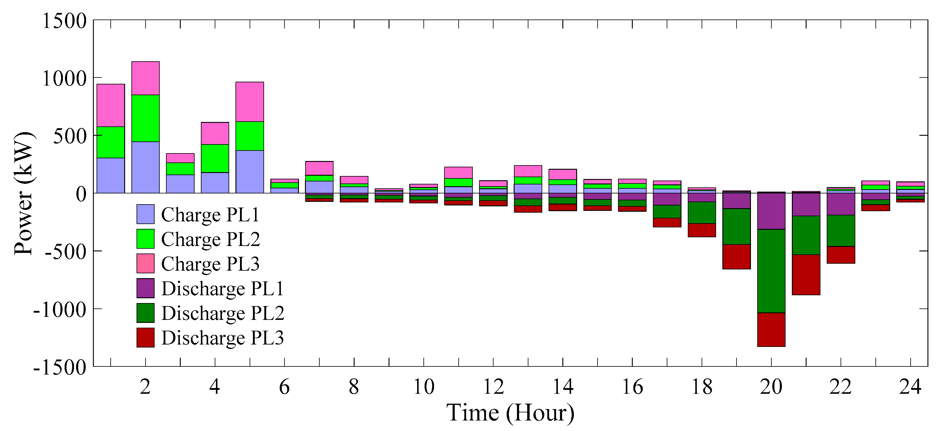
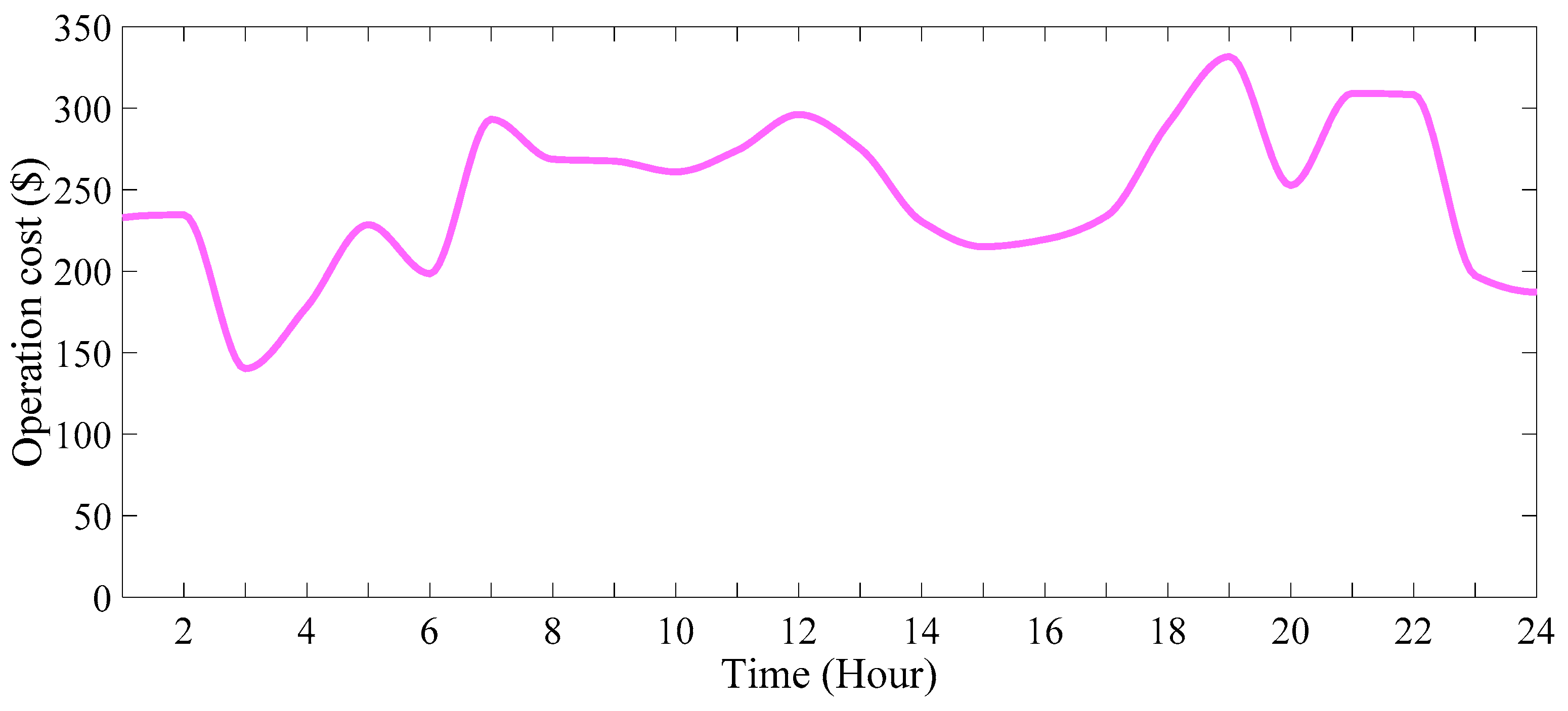
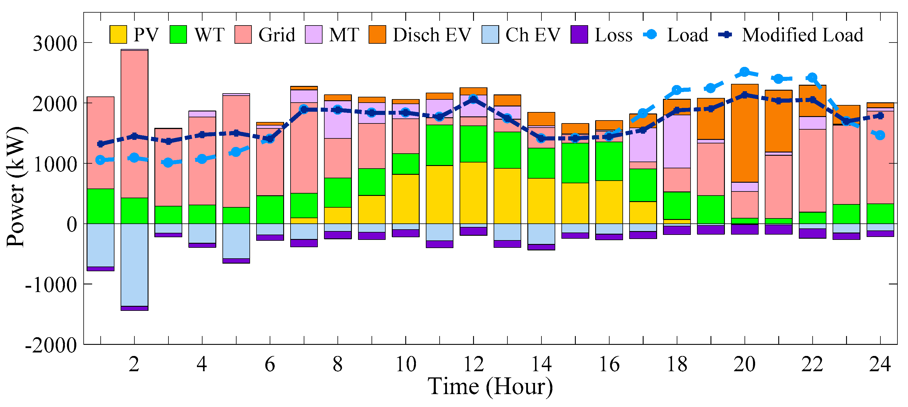
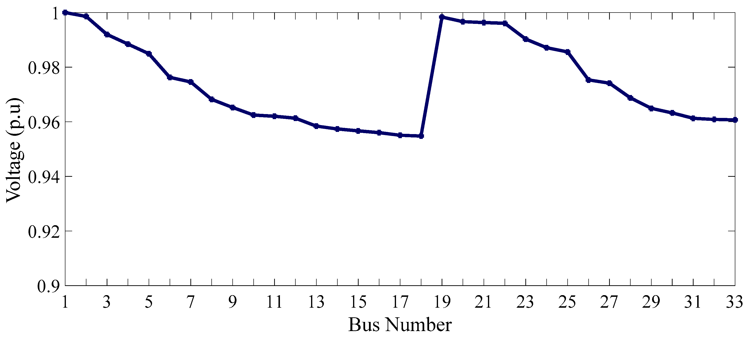
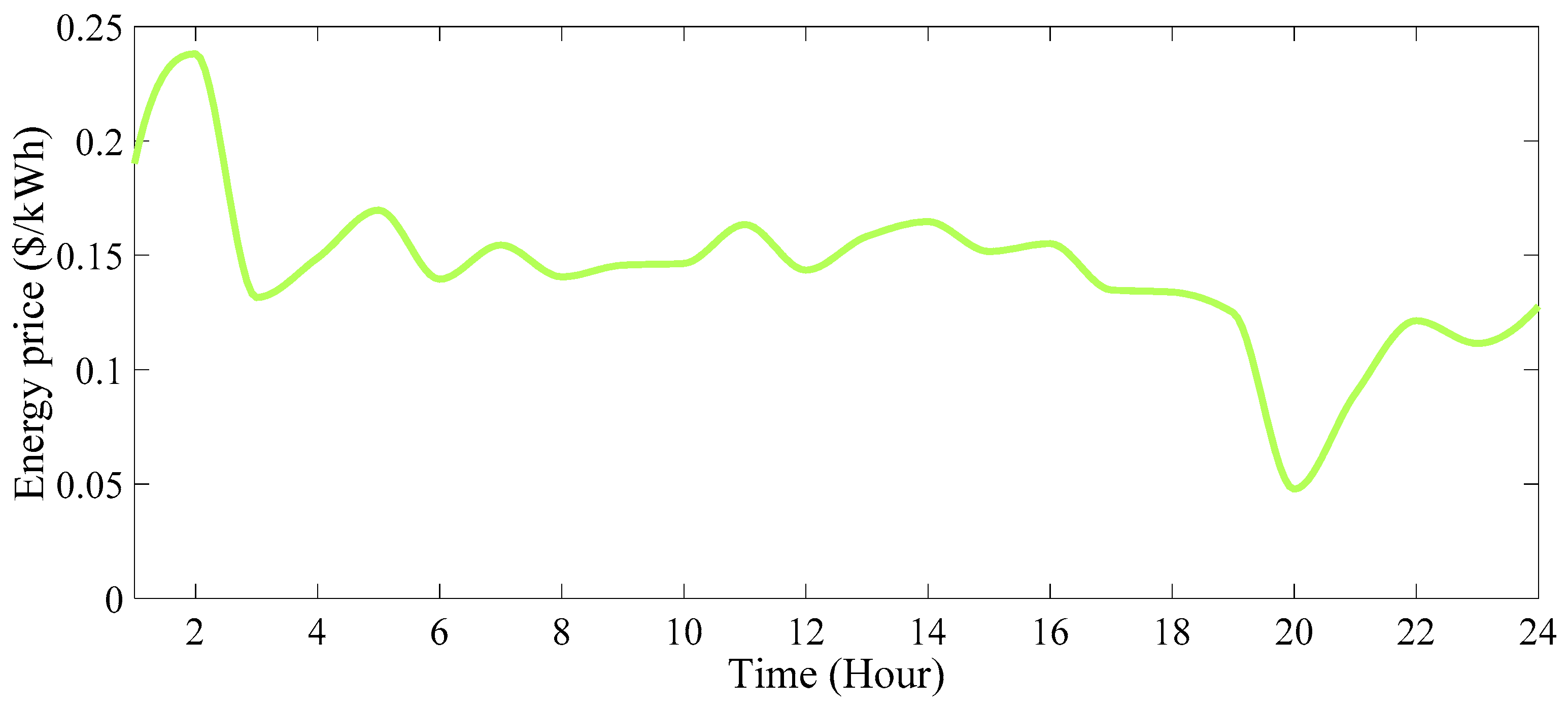
7.5. Results of Scenario 5
7.6. Scenario Comparison
8. Conclusions
- ➢
- The presence of EVPLs solely has improved technical and environmental indexes.
- ➢
- With the optimal allocation of DERs and EVPLs, in addition to the appropriate scheduling of EVs, all the techno-economic and environmental criteria of the network have been significantly improved.
- ➢
- The integration of the DRP alongside DERs and EVPLs can have an efficient effect on reducing the operation cost of the system and improving the power quality parameters of the network. Also, the implementation of the DRP can provide the basis for increasing the use of DERs and, as a result, reducing pollution emissions.
- ➢
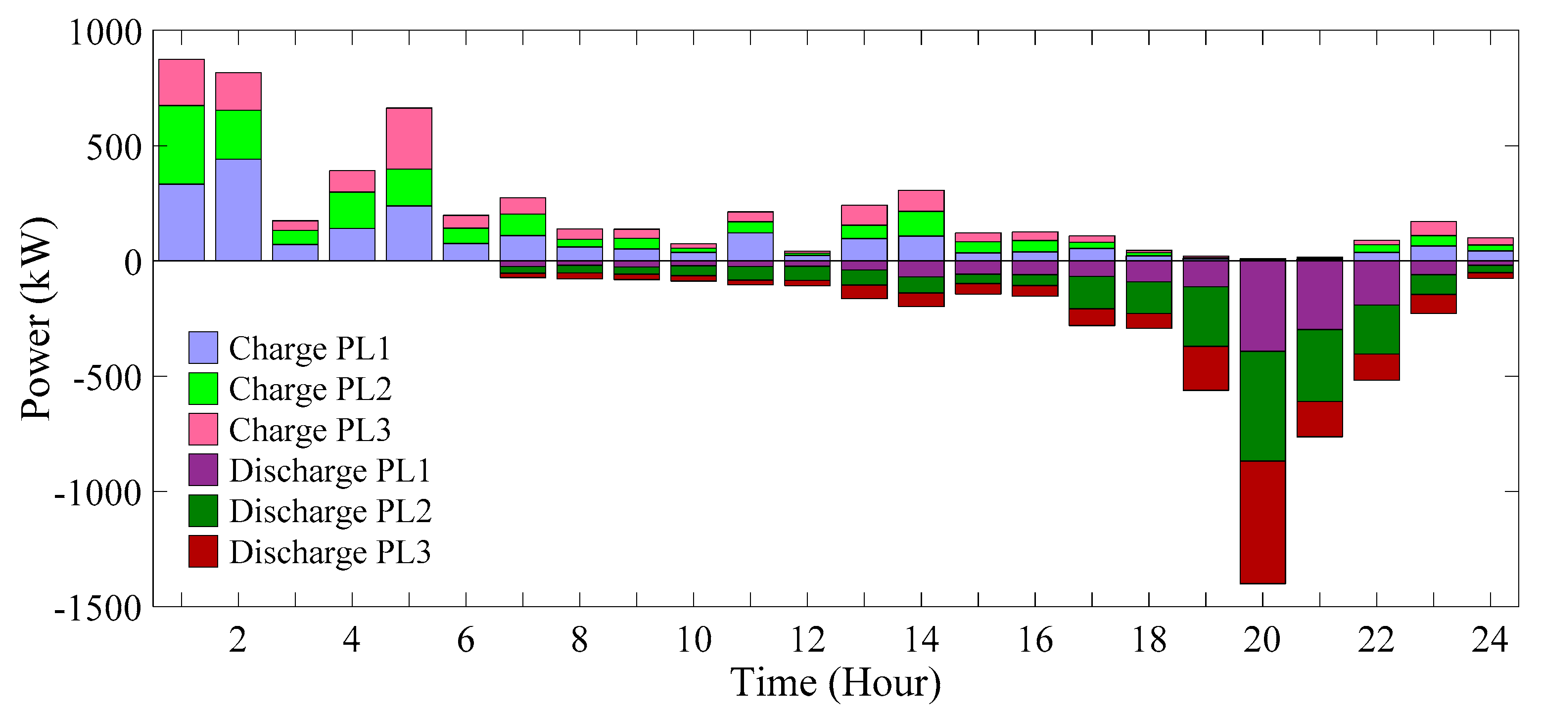
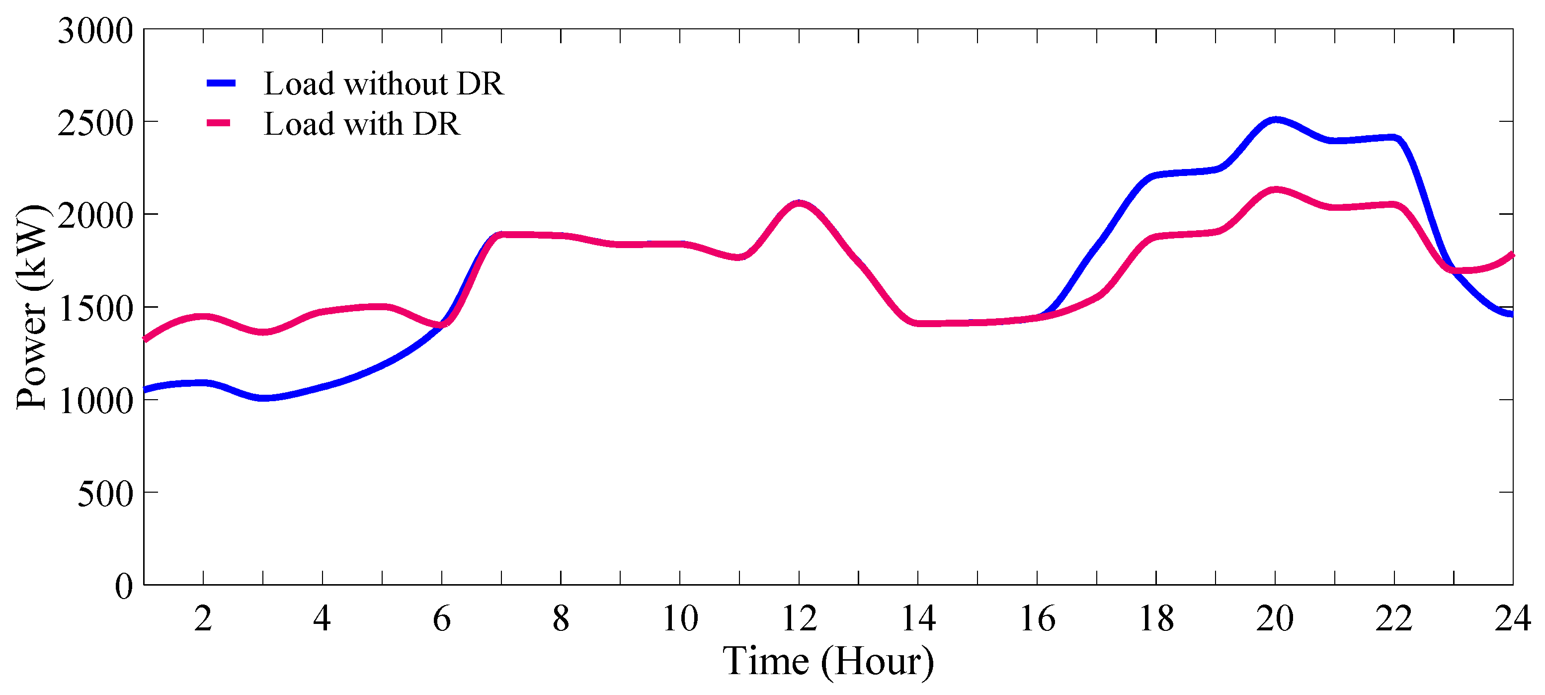
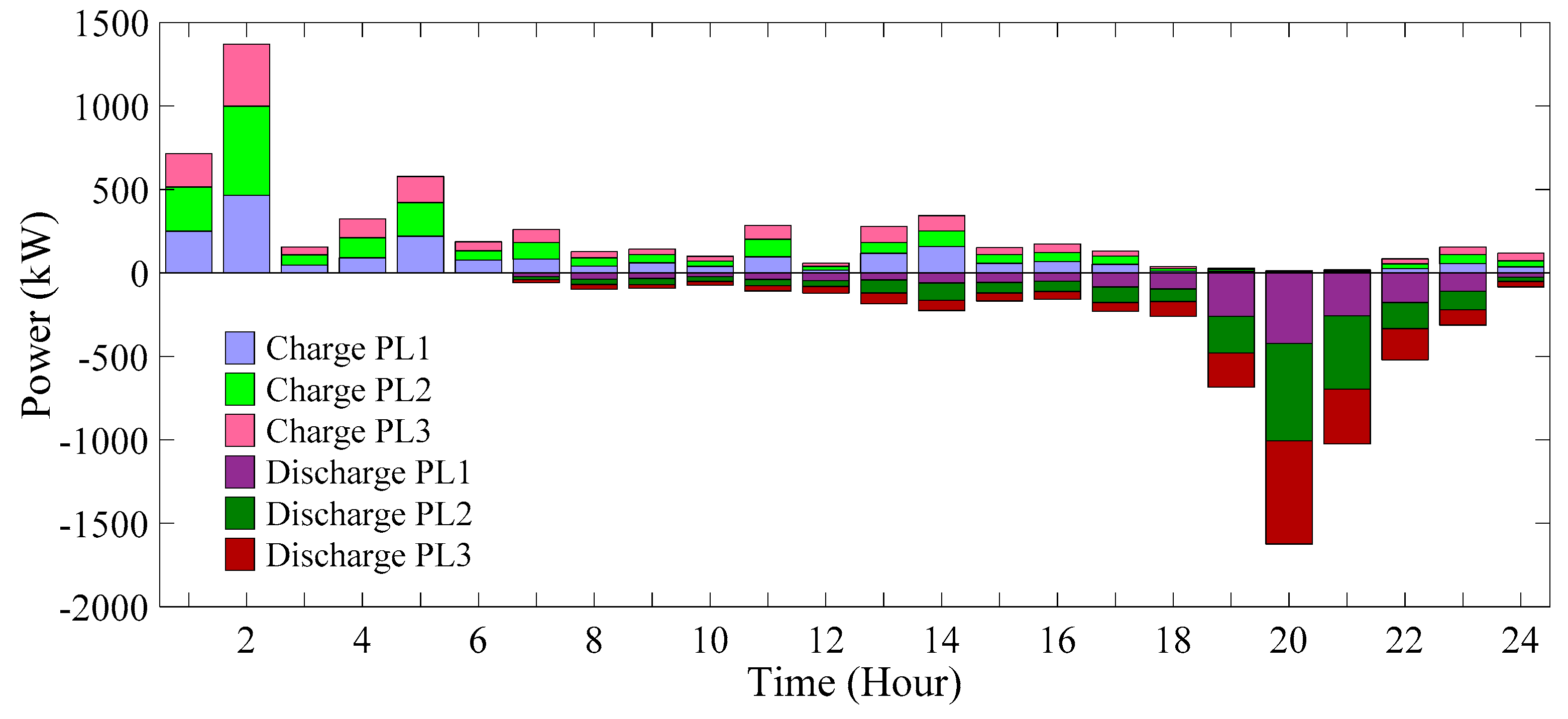
- In addition to flattening the load profile, charging EVs during off-peak periods and discharging them during on-peak hours will result in economic benefits for owners of EVs.
- ▪
- Investigating the effects of EVs and DGs on reactive power losses.
- ▪
- Considering the precise traffic model of EVs in the EVPL allocation and management area.
- ▪
- Determining the framework of the contract provisions between the PLs and the EVs, such as the penalty for the EV’s early departure from the PL or failure to provide the requested power by the PL, etc.
- ▪
- Allocation of PLs and DERs simultaneously with capacitors and other reactive power compensator devices such as static VAR compensators (SVC).
- ▪
- PL and DER energy management by considering the effect of different seasons on the technical and economic parameters of the studied issue.
- ▪
- Solving the problem of allocating PLs and DERs by considering the possibility of injecting reactive power into the network by EVs’ batteries, as well as RESs, and participating them in the reactive power management market.
Author Contributions
Funding
Data Availability Statement
Conflicts of Interest
Appendix A

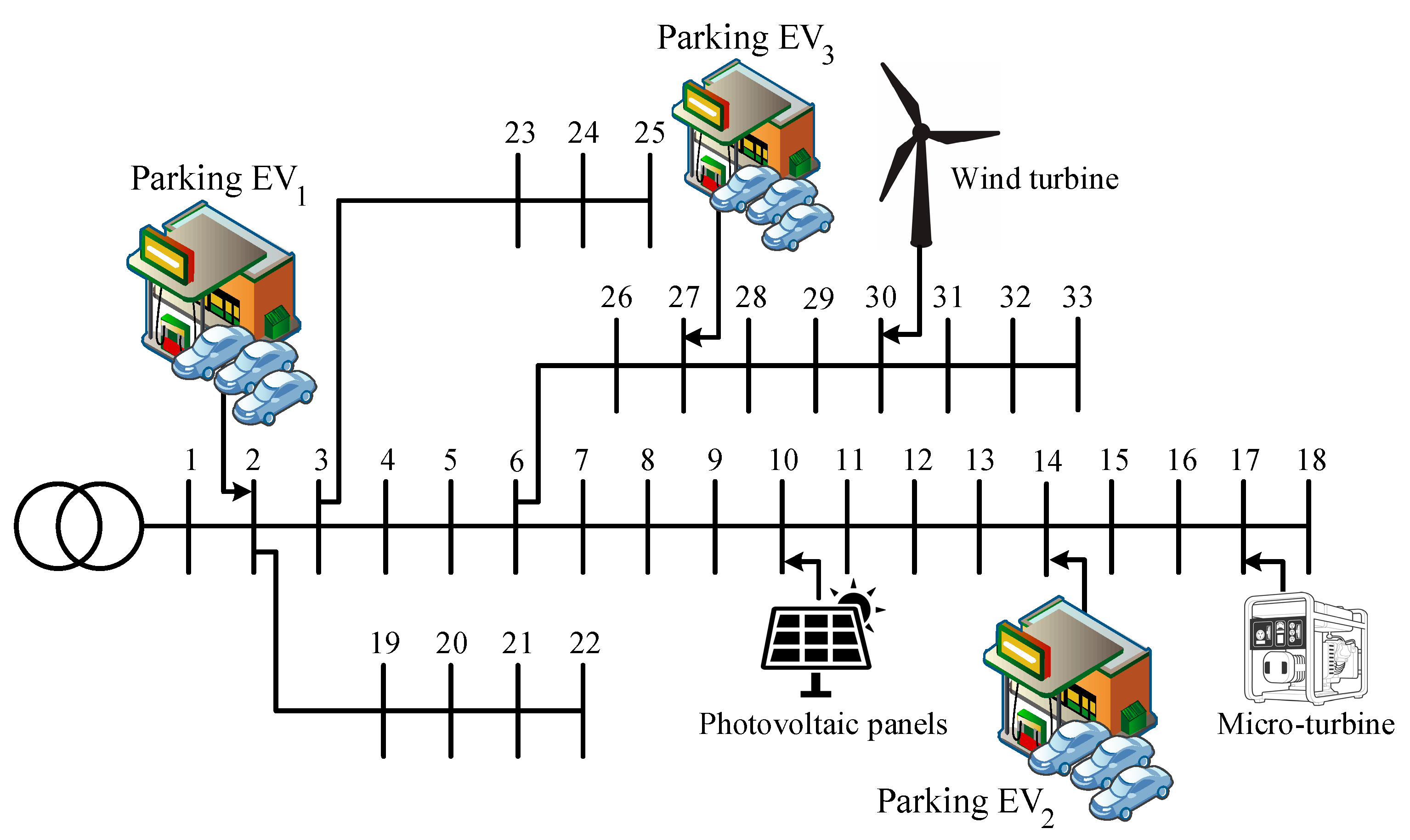
| Transmitter Bus | Receiver Bus | R(Ω) | X(Ω) | P (kW) | Q(kVar) |
|---|---|---|---|---|---|
| 1 | 2 | 0.0922 | 0.0470 | 100 | 60 |
| 2 | 3 | 0.4930 | 0.2511 | 90 | 40 |
| 3 | 4 | 0.3660 | 0.1864 | 120 | 80 |
| 4 | 5 | 0.3811 | 0.1941 | 60 | 30 |
| 5 | 6 | 0.8190 | 0.7070 | 60 | 20 |
| 6 | 7 | 0.1872 | 0.6188 | 200 | 100 |
| 7 | 8 | 0.7114 | 0.2351 | 200 | 100 |
| 8 | 9 | 1.0300 | 0.7400 | 60 | 20 |
| 9 | 10 | 1.0440 | 0.7400 | 60 | 20 |
| 10 | 11 | 0.1966 | 0.0650 | 45 | 30 |
| 11 | 12 | 0.3744 | 0.1238 | 60 | 35 |
| 12 | 13 | 1.4680 | 1.1550 | 60 | 35 |
| 13 | 14 | 0.5416 | 0.7129 | 120 | 80 |
| 14 | 15 | 0.5910 | 0.5260 | 60 | 10 |
| 15 | 16 | 0.7463 | 0.5450 | 60 | 20 |
| 16 | 17 | 1.2890 | 1.7210 | 60 | 20 |
| 17 | 18 | 0.7320 | 0.5740 | 90 | 40 |
| 2 | 19 | 0.1640 | 0.1565 | 90 | 40 |
| 19 | 20 | 1.5042 | 1.3554 | 90 | 40 |
| 20 | 21 | 0.4095 | 0.4784 | 90 | 40 |
| 21 | 22 | 0.7089 | 0.9373 | 90 | 40 |
| 3 | 23 | 0.4512 | 0.3083 | 90 | 50 |
| 23 | 24 | 0.8980 | 0.7091 | 420 | 200 |
| 24 | 25 | 0.8960 | 0.7011 | 420 | 200 |
| 6 | 26 | 0.2030 | 0.1034 | 60 | 25 |
| 26 | 27 | 0.2842 | 0.1447 | 60 | 25 |
| 27 | 28 | 1.0590 | 0.9337 | 60 | 20 |
| 28 | 29 | 0.8042 | 0.07006 | 120 | 70 |
| 29 | 30 | 0.5075 | 0.2584 | 200 | 600 |
| 30 | 31 | 0.9744 | 0.9630 | 150 | 70 |
| 31 | 32 | 0.3105 | 0.3619 | 210 | 100 |
| 32 | 33 | 0.3410 | 0.5302 | 60 | 40 |
| Pmax (kW) | Pmin (kW) | Selling Price (USD/kWh) | CO2 (kg/MWh) | SO2 (kg/MWh) | NOx (kg/MWh) | DG Type |
|---|---|---|---|---|---|---|
| 1500 | 10 | 0.125 | 720 | 0.0054 | 0.23 | Microturbine |
| 1000 | 0 | 0.153 | 0 | 0 | 0 | Wind turbine |
| 1500 | 0 | 0.153 | 0 | 0 | 0 | Photovoltaic |
| Cost Coefficients | Power Plant | ||
|---|---|---|---|
| c | b | a | Microturbine |
| 0.002 | 0.0133 | 10 | |
| C= 5/2 | K= 5/8 | vr = 12 m/s | vci = 3 m/s, vco = 25 m/s | Wind Turbine |
| Ꞃpv = 18 | Spv= 8000 m2 | K1 = 5.5, K2 = 6.8 | C1= 8/1, C2 = 2.6 | Photovoltaic |
| Value | Parameter | Value | Parameter |
|---|---|---|---|
| 26 | The mean of the normal distribution function of the initial charge (charge mode) | 20 | The standard deviation of the log-normal function () |
| 1/7 | The standard deviation of the normal distribution function of the initial charge (charge mode) | 40 | Mean of the log-normal function () |
| 72 | The mean of the normal distribution function of the initial charge (discharge mode) | 1 | The electric energy input to the battery |
| 2/6 | The standard deviation of the normal distribution function of the initial charge (discharge mode) | 7 | EV arrival time mean ( |
| 13/7 | The mean of the normal distribution function of the EV presence in the PLs | 1/73 | EV arrival time standard deviation () |
| 4/5 | The standard deviation of the normal distribution function of the EV’s presence in the PLs | 18 | EV departure time mean ( |
| 1 | The constant of EV energy consumption (β) | 1/73 | EV departure time standard deviation () |
| EV Type | Market Share (Percent) | BCAP (kWh) | α (kWh/mile) |
|---|---|---|---|
| 1 | 25 | 10 | 0/3790 |
| 2 | 25 | 12 | 0/4288 |
| 3 | 25 | 16 | 0/5740 |
| 4 | 25 | 21 | 0/8180 |
References
- Ravi, S.S.; Aziz, M. Utilization of Electric Vehicles for Vehicle-to-Grid Services: Progress and Perspectives. Energies 2022, 15, 589. [Google Scholar] [CrossRef]
- Ray, S.; Kasturi, K.; Patnaik, S.; Nayak, M.R. Review of electric vehicles integration impacts in distribution networks: Placement, charging/discharging strategies, objectives and optimisation models. J. Energy Storage 2023, 72, 108672. [Google Scholar] [CrossRef]
- Osório, G.J.; Gough, M.; Lotfi, M.; Santos, S.F.; Espassandim, H.M.; Shafie-Khah, M.; Catalão, J.P. Rooftop photovoltaic parking lots to support electric vehicles charging: A comprehensive survey. Int. J. Electr. Power Energy Syst. 2021, 133, 107274. [Google Scholar] [CrossRef]
- Bagherzadeh, L.; Shayeghi, H.; Pirouzi, S.; Shafie-Khah, M.; Catalão, J.P.S. Coordinated flexible energy and self-healing management according to the multi-agent system-based restoration scheme in active distribution network. IET Renew. Power Gener. 2021, 15, 1765–1777. [Google Scholar] [CrossRef]
- Afshar, S.; Macedo, P.; Mohamed, F.; Disfani, V. Mobile charging stations for electric vehicles—A review. Renew. Sustain. Energy Rev. 2021, 152, 111654. [Google Scholar] [CrossRef]
- Barman, P.; Dutta, L.; Bordoloi, S.; Kalita, A.; Buragohain, P.; Bharali, S.; Azzopardi, B. Renewable energy integration with electric vehicle technology: A review of the existing smart charging approaches. Renew. Sustain. Energy Rev. 2023, 183, 113518. [Google Scholar] [CrossRef]
- Vahidinasab, V.; Mohammadi-Ivatloo, B. Energy Systems Transition: Digitalization, Decarbonization, Decentralization and Democratization; Springer Nature: Berlin/Heidelberg, Germany, 2023. [Google Scholar]
- Zhao, B.; Duan, P.; Fen, M.; Xue, Q.; Hua, J.; Yang, Z. Optimal operation of distribution networks and multiple community energy prosumers based on mixed game theory. Energy 2023, 278, 128025. [Google Scholar] [CrossRef]
- Bagherzadeh, L.; Kamwa, I. Coupling Economic Energy Management and Flexibility Regulation of Power Systems with Renewable Energy Hubs Through Tso-Dso Coordination. Available online: https://ssrn.com/abstract=4508787 (accessed on 13 July 2023).
- Kamwa, I.; Bagherzadeh, L.; Delavari, A. Integrated Demand Response Programs in Energy Hubs: A Review of Applications, Classifications, Models and Future Directions. Energies 2023, 16, 4443. [Google Scholar] [CrossRef]
- Moradi, M.H.; Abedini, M.; Tousi, S.R.; Hosseinian, S.M. Optimal siting and sizing of renewable energy sources and charging stations simultaneously based on Differential Evolution algorithm. Int. J. Electr. Power Energy Syst. 2015, 73, 1015–1024. [Google Scholar] [CrossRef]
- Amini, M.H.; Moghaddam, M.P.; Karabasoglu, O. Simultaneous allocation of electric vehicles’ parking lots and distributed renewable resources in smart power distribution networks. Sustain. Cities Soc. 2017, 28, 332–342. [Google Scholar] [CrossRef]
- Moradijoz, M.; Ghazanfarimeymand, A.; Moghaddam, M.P.; Haghifam, M.R. Optimum placement of distributed generation and parking lots for loss reduction in distribution networks. In Proceedings of the 2012 17th Electrical Power Distribution Conference (EPDC), Tehran, Iran, 2–3 May 2012; pp. 1–5. [Google Scholar]
- Mozafar, M.R.; Moradi, M.H.; Amini, M.H. A simultaneous approach for optimal allocation of renewable energy sources and electric vehicle charging stations in smart grids based on improved GA-PSO algorithm. Sustain. Cities Soc. 2017, 32, 627–637. [Google Scholar] [CrossRef]
- Bagherzadeh, L.; Shayeghi, H.; Shenava, S.J.S. Optimal Allocation of Electric Vehicle Parking lots and Renewable Energy Sources Simultaneously for Improving the Performance of Distribution System. In Proceedings of the 2019 24th Electrical Power Distribution Conference (EPDC), Khoramabad, Iran, 20 June 2019; pp. 87–94. [Google Scholar]
- Luo, L.; Wu, Z.; Gu, W.; Huang, H.; Gao, S.; Han, J. Coordinated allocation of distributed generation resources and electric vehicle charging stations in distribution systems with vehicle-to-grid interaction. Energy 2019, 192, 116631. [Google Scholar] [CrossRef]
- Vijayalakshmi, V.J.; Arumugam, P.; Christy, A.A.; Brindha, R. Simultaneous allocation of EV charging stations and renewable energy sources: An Elite RERNN-m2MPA approach. Int. J. Energy Res. 2022, 46, 9020–9040. [Google Scholar] [CrossRef]
- Dharavat, N.; Sudabattula, S.K.; Velamuri, S.; Mishra, S.; Sharma, N.K.; Bajaj, M.; Elgamli, E.; Shouran, M.; Kamel, S. Optimal Allocation of Renewable Distributed Generators and Electric Vehicles in a Distribution System Using the Political Optimization Algorithm. Energies 2022, 15, 6698. [Google Scholar] [CrossRef]
- Kandil, S.M.; Farag, H.E.; Shaaban, M.F.; El-Sharafy, M.Z. A combined resource allocation framework for PEVs charging stations, renewable energy resources and distributed energy storage systems. Energy 2018, 143, 961–972. [Google Scholar] [CrossRef]
- da Silva, E.C.; Melgar-Dominguez, O.D.; Romero, R. Simultaneous Distributed Generation and Electric Vehicles Hosting Capacity Assessment in Electric Distribution Systems. IEEE Access 2021, 9, 110927–110939. [Google Scholar] [CrossRef]
- Tabatabaei, J.; Moghaddam, M.S.; Baigi, J.M. Rearrangement of Electrical Distribution Networks with Optimal Coordination of Grid-Connected Hybrid Electric Vehicles and Wind Power Generation Sources. IEEE Access 2020, 8, 219513–219524. [Google Scholar] [CrossRef]
- Shafie-Khah, M.; Siano, P.; Fitiwi, D.Z.; Mahmoudi, N.; Catalao, J.P. An innovative two-level model for electric vehicle parking lots in distribution systems with renewable energy. IEEE Trans. Smart Grid 2017, 9, 1506–1520. [Google Scholar] [CrossRef]
- Bagherzadeh, L.; Shayeghi, H.; Seyed-Shenava, S.-J. Optimal Allocation of Electric Vehicle Parking Lots for Minimizing Distribution System Costs Considering Uncertainties. In Proceedings of the 2019 Iranian Conference on Renewable Energy & Distributed Generation (ICREDG), Tehran, Iran, 11–12 June 2019; pp. 1–6. [Google Scholar]
- Shayanfar, H.; Shayeghi, H.; Bagherzadeh, L. Optimal Allocation of Electric Vehicle Parking Lots for Improving the Efficiency of Distribution System. In Proceedings of the 2019 International Conference on Artificial Intelligence (ICAI), Xuzhou, China, 22–23 August 2019; pp. 116–122. [Google Scholar]
- Aljeddani, S.M.; Mohammea, M. A novel approach to Weibull distribution for the assessment of wind energy speed. Alex. Eng. J. 2023, 78, 56–64. [Google Scholar] [CrossRef]
- Bagherzadeh, L.; Shahinzadeh, H.; Shayeghi, H.; Gharehpetian, G.B. A short-term energy management of microgrids considering renewable energy resources, micro-compressed air energy storage and DRPs. Int. J. Renew. Energy Res. 2019, 9, 1712–1723. [Google Scholar]
- Afridi, M.; Tatapudi, S.; Flicker, J.; Srinivasan, D.; Tamizhmani, G. Reliability evaluation of DC power optimizers for photovoltaic systems: Accelerated testing at high temperatures with fixed and cyclic power stresses. Eng. Fail. Anal. 2023, 152, 107484. [Google Scholar] [CrossRef]
- Bagherzadeh, L.; Shahinzadeh, H.; Gharehpetian, G.B. Scheduling of Distributed Energy Resources in Active Distribution Networks Considering Combination of Techno-Economic and Environmental Objectives. In Proceedings of the 2019 International Power System Conference (PSC), Tehran, Iran, 30 December 2019; pp. 687–695. [Google Scholar]
- Rizvi, M.; Pratap, B.; Singh, S.B. Demand-side management in microgrid using novel hybrid metaheuristic algorithm. Electr. Eng. 2023, 105, 1867–1881. [Google Scholar] [CrossRef]
- Mirjalili, S.; Gandomi, A.H.; Mirjalili, S.Z.; Saremi, S.; Faris, H.; Mirjalili, S.M. Salp Swarm Algorithm: A bio-inspired optimizer for engineering design problems. Adv. Eng. Softw. 2017, 114, 163–191. [Google Scholar] [CrossRef]
- Chinchanikar, S.; Shinde, S.; Shaikh, A.; Gaikwad, V.; Ambhore, N.H. Multi-objective Optimization of FDM Using Hybrid Genetic Algorithm-Based Multi-criteria Decision-Making (MCDM) Techniques. J. Inst. Eng. India Ser. D 2023, 1–15. [Google Scholar] [CrossRef]


| Scenario 2 | MT | WT | PV |
|---|---|---|---|
| Location | 15 | 30 | 10 |
| Capacity (kW) | 1462.713 | 667.051 | 823.713 |
| Scenario 3 | PL1 | PL2 | PL3 |
|---|---|---|---|
| Location | 2 | 19 | 22 |
| Capacity (KW) | 2251.12 | 1700.745 | 1653.25 |
| Scenario 4 | MT | WT | PV | PL1 | PL2 | PL3 |
|---|---|---|---|---|---|---|
| Location | 17 | 30 | 10 | 2 | 14 | 27 |
| Capacity (kW) | 1073.571 | 686.023 | 832.349 | 2312.316 | 1800.812 | 1906.798 |
| Scenario 5 | MT | WT | PV | PL1 | PL2 | PL3 |
|---|---|---|---|---|---|---|
| Location | 18 | 33 | 15 | 2 | 10 | 30 |
| Capacity (kW) | 887.536 | 692.013 | 1103.053 | 2512.73 | 2102.46 | 2001.53 |
| Results | Scenario 1 | Scenario 2 | Scenario 3 | Scenario 4 | Scenario 5 |
|---|---|---|---|---|---|
| The cost of energy transported from the upstream network (USD) | 6023.404 | 2942.218 | 5884.27 | 2350.442 | 2094.191 |
| The cost of providing energy by WT (USD) | 0 | 1495.542 | 0 | 1439.542 | 1456.585 |
| The cost of providing energy by PV (USD) | 0 | 916.209 | 0 | 972.2091 | 1056.555 |
| The cost of providing energy by MT (USD) | 0 | 640.116 | 0 | 578.0892 | 572.8952 |
| The cost of EVPL charging (USD) | 0 | 0 | 634.3372 | 642.5634 | 696.3363 |
| The revenue of EVPL discharging (USD) | 0 | 0 | 1130.619 | 984.6014 | 1004.242 |
| The cost of greenhouse gas emissions (USD) | 386.7665 | 222.677 | 376.7547 | 211.9482 | 204.7329 |
| Power losses (kW) | 4061.6 | 3002.41 | 3752.24 | 2737.637 | 2658.71 |
| Voltage deviation (p.u) | 1.8283 | 1.3006 | 1.6808 | 0.9966 | 0.8244 |
| Total operation cost of the system (USD) | 6410.171 | 6216.762 | 6757.306 | 5894.269 | 5692.865 |
| The average operation cost of the system (USD/h) | 267.0904 | 259.0317 | 281.5544 | 245.5945 | 237.2027 |
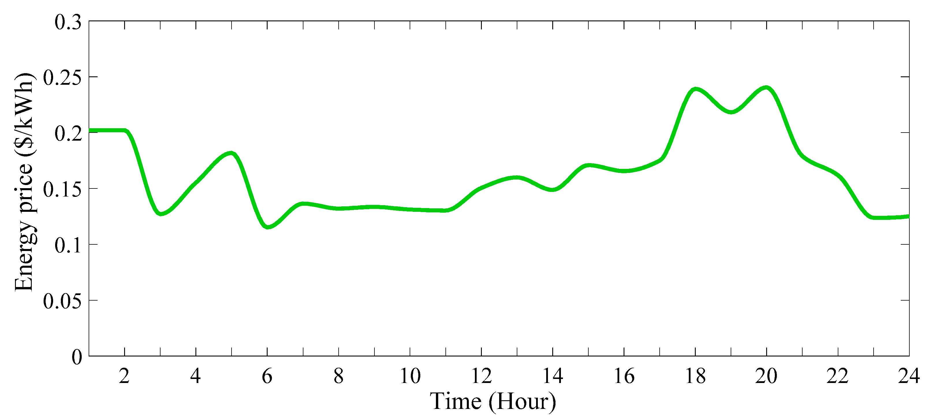
| The average price of electricity (USD/kWh) | 0.14956 | 0.147466 | 0.162714 | 0.14986 | 0.14306 |
Disclaimer/Publisher’s Note: The statements, opinions and data contained in all publications are solely those of the individual author(s) and contributor(s) and not of MDPI and/or the editor(s). MDPI and/or the editor(s) disclaim responsibility for any injury to people or property resulting from any ideas, methods, instructions or products referred to in the content. |
© 2023 by the authors. Licensee MDPI, Basel, Switzerland. This article is an open access article distributed under the terms and conditions of the Creative Commons Attribution (CC BY) license (https://creativecommons.org/licenses/by/4.0/).
Share and Cite
Bagherzadeh, L.; Kamwa, I. Joint Multi-Objective Allocation of Parking Lots and DERs in Active Distribution Network Considering Demand Response Programs. Energies 2023, 16, 7805. https://doi.org/10.3390/en16237805
Bagherzadeh L, Kamwa I. Joint Multi-Objective Allocation of Parking Lots and DERs in Active Distribution Network Considering Demand Response Programs. Energies. 2023; 16(23):7805. https://doi.org/10.3390/en16237805
Chicago/Turabian StyleBagherzadeh, Leila, and Innocent Kamwa. 2023. "Joint Multi-Objective Allocation of Parking Lots and DERs in Active Distribution Network Considering Demand Response Programs" Energies 16, no. 23: 7805. https://doi.org/10.3390/en16237805