A Neural Network-Based Method for Real-Time Inversion of Nonlinear Heat Transfer Problems

Abstract

Inverse heat transfer problems are important in numerous scientific research and engineering applications. This paper proposes a network-based method utilizing the nonlinear autoregressive with exogenous inputs (NARX) neural network, which can achieve real-time identification of thermal boundary conditions for nonlinear transient heat transfer processes. With the introduction of the NARX neural network, the proposed method offers two key advantages: (1) The proposed method can obtain inversion results using only surface temperature time series. (2) The heat flux can be estimated even when the state equation of the system is unknown. The NARX neural network is trained using the Bayesian regularization algorithm with a dataset comprising exact surface temperature and heat flux data. The neural network takes current and historical surface temperature measurements as inputs to calculate the heat flux at the current time. The capability of the NARX method has been verified through numerical simulation experiments. Experimental results demonstrate that the NARX method has high precision, strong noise resistance, and broad applicability. The composition of the input data, the surface temperature measurement noise, and the boundary heat flux shape have been studied in detail for their impact on the inversion results. The NARX method is a highly competitive solution to inverse heat transfer problems.

1. Introduction

Heat transfer is a fundamental physical phenomenon that influences numerous scientific research and industrial processes. In a forward heat transfer problem, the temperature fields can be obtained with the initial and boundary conditions using the governing heat equations. Researchers have proposed many analytical and numerical methods to solve the forward problem [1,2,3,4]. However, when the unknown boundary conditions need to be inversed from specific temperature measurement data, it becomes an inverse heat conduction problem (IHCP). Inverse problems are common in various fields, including power generation [5,6], spacecraft protection [7,8,9,10,11], metal processing [12,13,14], chip cooling [15,16], and biomedicine [17]. Inverse heat conduction problems are ill-posed, meaning a stable solution cannot be obtained analytically [18]. Minor errors in temperature measurement information can lead to divergence in the inversion results.

In recent decades, researchers have developed many effective methods to address the inverse heat transfer problem. These solutions can be broadly classified into two categories based on the type of required inputs: whole-domain algorithms and sequential algorithms. The whole-domain algorithm requires all measurement information from the start to the termination of the time domain to simultaneously inverse the values of the unknown parameters throughout the entire time domain. Tikhonov [19] developed a regularization method for solving the inverse problem, which fundamentally aims to enhance the reliability of the results by introducing a stable function and regularization parameters. The selection of regularization parameters significantly influences the accuracy of the inversion results, posing a challenge for its application in IHCPs. Okamoto [20] employed an L-curve method to select optimal regularization parameters and developed an algorithm to make an inversion in the solidification process using the Tikhonov regularization method. Huang [21] utilized a steepest descent method (SDM) to identify the transient heat flux in a motor. Cui [22] applied the Levenberg–Marquard method to inverse the boundary heat flux in a two-dimensional transient heat conduction process, achieving commendable results. The whole-domain algorithms are incapable of performing real-time inversion due to the requirement for measurement information from the entire time domain and numerous forward iterations to approximate values of unknown parameters. Therefore, it cannot satisfy the demand for real-time inversion in certain practical application scenarios.

The sequential algorithms utilize known temperature measurements at the current moment to inverse the unknown parameters in chronological order. Compared with the whole-domain algorithms, the sequential algorithms can perform real-time inversion of parameters at the current moment without information from the entire time domain, thus requiring less computational power. Numerous sequential algorithms have been proposed by researchers, including the sequential function specification method (SFSM) [23], digital filter method [24], Kalman filter algorithm [10,11], and proportional integral derivative (PID) algorithm [25,26]. Back [23] proposed the SFSM for the estimation of unknown parameters at the current time based on the temperature measurements over a future period. The SFSM has been widely applied to inverse heat transfer problems. Mohammadiun [27] used the SFSM to identify the heat flux on the boundary of sintered material and investigated the influences of different measurement positions and the number of time steps on the identification results. The SFSM requires assumptions about the function form of the unknown parameters in future time, making the estimation results very sensitive to future time steps and function form assumptions. This is the biggest challenge faced by SFSM. Najafi [24] developed a digital filter method to achieve near real-time inversion in multi-layer material heat transfer problems with temperature measurements from two points inside the material. Wen [11] utilized Unscented Kalman Filter technology to perform real-time inversion of surface thermal conditions in spacecraft thermal protection systems, achieving good accuracy when material thermal properties change with temperature. Hong [10] combined the extended Kalman filtering and Rauch–Tung–Striebel smoother to calculate the time-variant heat flux and interior temperature fields in thermal protection systems. Wan [25] developed an algorithm based on PID control theory that can predict transient boundary heat flux. Experimental results demonstrate that the PID algorithm has a good anti-disturbance ability. Huang [26] developed a real-time solution for unsteady IHCP based on the PID algorithm that enhanced by the improved whale optimization algorithm. Significant progress has been achieved in solving inverse heat conduction problems using sequential algorithms. However, most current methods require assumptions about future values of unknown parameters or the state equation of the system, limiting the application of these algorithms in some practical problems.

Machine learning is a method that has received widespread attention and practical application, and the artificial neural network (ANN) is an important category within it. ANNs can simulate the structure and operation of the biological brain, which enable it to fit any nonlinear relationship, demonstrating robustness and wide applicability. Therefore, ANN is a competitive solution for IHCPs, especially when the accurate mathematical model of the system is challenging to obtain. Deng [28] used a back propagation neural network (BPNN) to predict the unidentified heat flux with temperature measurements from multiple points inside the object. The BPNN is enhanced with the Bayesian regularization algorithm. Najafi [29] utilized an ANN as a digital filter and achieved an approximate real-time estimation of surface thermal conditions based on temperature measurements from past and future time steps. Lohner [30] applied the ANN to achieve the inversion of nonlinear heat transfer problems and compared the results with those from interpolation algorithms, finding that the ANN method provided more accurate results. Wan [31] combined the PID algorithm with a single neuron to automatically adjust the PID tuning parameters. This method can achieve online prediction of heat flux in a one-dimensional heat conduction problem. While significant progress has been made in using artificial neural networks for IHCPs, a common obstacle with many methods is their requirement for multiple sensors inside the object, which can be challenging to implement in various scenarios. The nonlinear autoregressive with exogenous inputs (NARX) neural network, a dynamic network that incorporates delay and feedback mechanisms, offers a potential solution. Despite its relatively limited application in heat transfer problems, the capability of the NARX neural network to recall historical data places it as a potential approach for solving IHCPs without the requirement of multiple internal temperature sensors.

This study proposed a boundary heat flux identification algorithm based on the NARX neural network. The unique structure of the NARX neural network enables this algorithm to identify boundary heat flux in real time in nonlinear heat conduction problems. This estimation is achieved using only surface temperature measurement data, eliminating the need for multiple temperature measurement points within the material or additional information about future parameters. The NARX neural network is trained using the Levenberg–Marquardt method and the Bayesian regularization algorithm. The inputs are the time series of temperature, and the output is the current boundary heat flux. The feasibility of this method has been verified through simulation experiments. The results demonstrate that the NARX method possesses adaptive ability, robust anti-interference capability, and broad applicability. It holds significant potential for practical scientific research and engineering applications.

2. Physical Model

In this study, a one-dimensional heat conduction problem is analyzed. The schematic illustration is depicted in Figure 1. It can serve as a simplified model for various practical engineering applications, such as thermal protection systems and boiler firewalls. It is assumed that the transient heat flux q(t) is loaded on the boundary at x = 0 and the right boundary at x = L is adiabatic. The governing equations [32] can be given as follows:

$$\frac{1}{\alpha }\frac{\partial T(x,t)}{\partial t}=\frac{{\partial }^{2}T(x,t)}{\partial x^2}, 0<x<L, t>0$$

(1)

where α = λ/ρc_p represents the thermal diffusivity.

In the modern view of material science, the internal structure of the materials changes at different temperatures [33]. So, the values of the thermal–physical properties vary with the change in temperature, which introduce nonlinearity in this problem. In this study, the slab is made of copper, and the precise properties values obtained by experiments at different temperatures are included in

Table 1. Thermal properties of copper [34].

T (K)	ρ (kg/m3)	cp (kJ/kg)	λ (W/m∙K)
100	9009	0.254	480
150	8992	0.323	429
200	8973	0.357	413
250	8951	0.377	406
300	8930	0.386	401
400	8884	0.396	393
600	8787	0.431	379
800	8642	0.448	366
1000	8568	0.446	352
1200	8548	0.480	339

. The thermal–physical properties at temperatures not listed in the table will be estimated using linear interpolation methods.

The initial and boundary conditions [32] are the following:

$$T\left(x,t=0\right)=T^0\left(x\right), 0\le x\le L$$

(2)

$${\left.-\lambda \frac{\partial T}{\partial t}\right|}_{x=0}=q\left(t\right)$$

(3)

$${\left.-\lambda \frac{\partial T}{\partial t}\right|}_{x=L}=0$$

(4)

The time-varying temperature fields can be calculated using the Equations (1)–(4) in forward heat conduction problem. In this study, a finite difference method with an explicit scheme [32] is utilized for the direct problem. The governing equations are discretized in the temporal domain and spatial domain, and the grids are depicted in Figure 2. The discrete equations are as follows:

$$T_0^k=T_0^{k-1}+\frac{2\alpha \mathsf{\Delta }t}{\mathsf{\Delta }{x}^2}\left[T_1^{k-1}-T_0^{k-1}+\frac{\mathsf{\Delta }x}{\lambda }{q}^{k-1}\right]$$

(5)

$$T_i^k=T_i^{k-1}+\frac{\alpha \mathsf{\Delta }t}{\mathsf{\Delta }{x}^2}\left[T_{i+1}^{k-1}-2T_i^{k-1}+T_{i-1}^{k-1}\right] i=\mathrm{1,2},\dots ,N-1$$

(6)

$$T_N^k=T_N^{k-1}+\frac{2\alpha \mathsf{\Delta }t}{\mathsf{\Delta }{x}^2}\left[T_{N-1}^{k-1}-T_N^{k-1}\right]$$

(7)

where T_i^k denotes the temperature at spatial node i at time node t_k; q^k−1 is the heat flux imposed to the boundary from t_k − 1 to t_k; ∆x is the spatial step size and N is the number of spatial nodes, N = L/∆x; ∆t is the time step size, t_k = kΔt, k = 1, 2, …, M; M is the number of temporal nodes, and M = T_total/∆t.

For inverse problems, the boundary heat flux is an unidentified parameter that needs to be estimated using the temperature measurements. The boundary heat flux can be calculated using the inner temperature fields with Fourier’s law. However, in most practical applications, the internal temperature fields cannot be measured. Therefore, the boundary heat flux needs to be estimated utilizing the measured data of surface temperature. As a result of the existence of internal heat conduction, changes in surface temperature can reflect the temperature fields within the object. The relationship between the transient boundary heat flux and surface temperature measurements can be expressed as a function:

$$q^k=f(T^0,\dots ,T^k,\mathrm{P}\mathrm{O}\mathrm{M})$$

(8)

where T⁰, …, T^k represent the surface temperature from the beginning to the moment k. The term POM means the properties of matter, including density, specific heat capacity, thermal conductivity, and slab thickness. ‘f’ represents a function that needs to be determined. In the current study, a NARX neural network is applied to fit the function ‘f’.

3. NARX Neural Network for Boundary Heat Flux Estimation

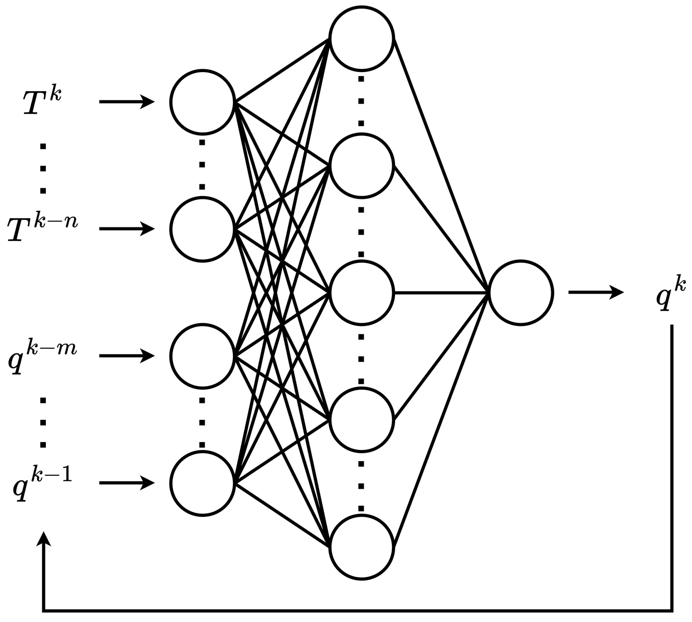
3.1. Mapping the NARX Neural Network Structure

A NARX neural network is employed to estimate the boundary heat flux in the current study. The structure of the network is depicted in Figure 3. The NARX neural network takes the discretized time series of surface temperature measurements and boundary heat flux as inputs. The discrete interval between input data is consistent with the sampling period of the measurement instrument:

$$\mathsf{\Delta }t=T^k-T^{k-1}=\frac{1}{fs}$$

(9)

where fs is the sampling rate. For the NARX neural network used in the current study, the time series of temperature, [T^k, T^k−1, …, T^k-n], are directly measured at the measurement point, while the time series of heat flux, [q^k-m, …, q^k−1], are obtained from the output values of the network on time steps earlier. The temporal relationship between the discrete temperature measurement and heat flux data is depicted in Figure 4.

The unique structure of the NARX neural network allows it to remember and utilize historical data to make predictions. This feature enables the network to use only surface temperature measurements as inputs and identify the boundary heat flux by fitting the relationship of surface temperature changes and heat flux without the requirements of temperature measurements inside the material or other inputs. This gives the NARX neural network a significant advantage for the inversion of heat conduction problems in real-world applications.

The NARX neural network is composed of multiple interconnected neurons, which are organized into three distinct layers: the input layer, the hidden layer, and the output layer. In the NARX neural network utilized in this study, the number of neurons in the input layer is the same as the dimension of the inputs. The hidden layer consists of 20 neurons, while the output layer contains a single neuron, which means that the output of this network is a single value. The nodes of each layer are interconnected with all nodes of the adjacent layers with certain weights.

The output of the network, y = q^k, can be obtained by following equations [28]:

$$o_j=S\left(\sum _i{w}_{ij}{x}_i+b_j\right)$$

(10)

$$y=\sum _j{w}_j{o}_j+b_y$$

(11)

where w is the weight of the connections between nodes, b is the bias, o is the output of the hidden layer, and S represents the Sigmoid activation function. The calculation process and parameters establish the relationship between the boundary heat flux and surface temperature measurements.

3.2. Network Training

The NARX neural network can be treated as a solution to the inverse heat conduction problem after a training process. The network will be trained in an open-loop state, which means the values of the heat flux in the input data are derived from the training data set, rather than the historical outputs of the network. The training procedure is a supervised learning process that provides the NARX neural network with the precise values of temperature and heat flux in the training dataset as inputs and compares the output values calculated by the network with the precise values in the training dataset. The purpose of the training procedure is to minimize the value of the loss function to the lowest by updating the weights, w, and the biases, b, in each iteration. The loss function utilized in this paper is the least squares criterion:

$$loss=\frac{1}{2}\sum _{k=t}^{t-n}{\left(q_{est}^k-q_{exa}^k\right)}^2=\frac{1}{2}\sum _{k=t}^{t-n}{e}_k^2$$

(12)

The weights and biases are adjusted in each iteration using the Levenberg–Marquardt algorithm [35] during the training process:

$${\mathbf{w}}^{k+1}={\mathbf{w}}^k-\mathsf{\kappa }{\left({\mathbf{J}}^T\mathbf{J}+\mu \mathbf{I}\right)}^{-1}\nabla f\left({\mathbf{w}}^k\right)$$

(13)

where κ is the learning rate, μ represents a regulating parameter, J is the Jacobian matrix, I is the identity matrix, and ∇f(w) is the gradient matrix.

When dealing with large training datasets and complex problems, the stability of the training results can be enhanced by a regularization algorithm. The Bayesian regularization algorithm [36] is employed in this paper. This algorithm involves augmenting the objective function with a regularization term, modifying the function to:

$$F={\xi }_1{E}_d+{\xi }_2{E}_w$$

(14)

$$E_d=\sum _{k=t}^{t-n}{e}_k^2$$

(15)

$$E_w=\sum _i{w}_i$$

(16)

Here, E_d represents the sum of squares of the deviations, E_w is the regularization term, and ξ₁ and ξ₂ are adjusting parameters. The introduction of the regularization term improves the network’s precision and simplifies its complexity. The training process is iterative. It commences with the Levenberg–Marquardt algorithm, using initial values of ξ₁ and ξ₂. Subsequently, the Bayesian regularization algorithm updates the values of ξ₁ and ξ₂, and training resumes with the L-M algorithm. This process repeats until the objective function falls below a predetermined threshold. After the training process, the parameters and structure of the NARX neural network are fixed. The trained network can be regarded as a function representing the boundary heat flux and surface temperature measurement values.

3.3. The Estimation Procedure

The NARX neural network developed in the current study can make an estimation of transient boundary heat flux in a nonlinear one-dimensional heat conduction problem. The procedure of this method is summarized as follows:

(1)

Train the NARX neural network with the training dataset, which consists of accurate heat flux and temperature data measured in experiments.

(2)

Provide the trained neural network with the initial input values, x⁰.

(3)

Calculated the initial output value of heat flux, q⁰, using Equations (10) and (11). Set k = 1.

(4)

Combine the historical outputs of heat flux obtained by the network and the time series of temperature measurements to form the inputs of the network, x^k.

(5)

Calculated the output value of heat flux, q^k by Equations (10) and (11).

(6)

If k equals the number of time steps that need to be inverted, stop this procedure, otherwise, set k = k + 1 and return to Step (4).

4. Results and Discussion

4.1. Simulation Experiment Conditions

For solving inverse heat transfer problems, the NARX neural network offers the advantage of being capable of inversing the boundary heat flux with only the time series of surface temperature measurements, due to its unique structure. To test and verify the accuracy and applicability of this method, one-dimensional heat conduction simulations are established in this study. In each experiment, a copper slab, with the thickness L = 1 cm and initial temperature T⁰ = 20 °C, is insulated at the boundary x = L, and exposed to a time-dependent heat flux q(t) at x = 0. These parameters are set to simulate most scenarios in practical applications [31]. The thermal physical parameters of the materials, which are time-dependent, are detailed in Table 1. The location of measurement is at x = L. The precise temperature fields are calculated using a numerical method. In this study, a computer powered by an Intel^® Xeon^® Gold 5117M CPU operating at 2.00 GHz is employed for computations. Given the computational power constraints and the precision demands of the forward heat transfer problem, the spatial step size is set to 0.001 cm, while the temporal step size is set to 0.1 s. The measurement sampling rate, fs, is 1 Hz, which is consistent with the common instrument sampling rate in industrial applications [37].

In practical engineering applications, measurement noise is inevitable due to reasons such as the precision of measuring instruments. In order to verify the anti-noise ability of the NARX method in practical applications, the noise was artificially added to the temperature measurement data in the simulation experiment:

$$T_{mea}^k=T_{exa}^k+\sigma \omega$$

(17)

where T^k_exa represents the exact temperature obtained by numerical calculation. σ is the standard deviation of the measurement noise, and ω is a random number following a standard normal distribution. In most engineering applications, it is particularly suited to describe the measurement noise using normal distribution. The normal distribution predicts that the scatter seen in measurement data will be distributed symmetrically about some central tendency [37].

In order to quantitatively assess the accuracy of the NARX method, the average root mean square error and the average relative error are brought in:

$$S_q=\sqrt{\frac{1}{M-1}\sum _{k=1}^M{\left[q_{est}^k-q_{exa}^k\right]}^2}$$

(18)

$${\eta }_{q,ave}=\frac{S_q}{\sqrt{\frac{1}{M-1}{\sum }_{k=1}^M{\left[q_{exa}^k\right]}^2}}$$

(19)

The training data of the NARX neural network consists of a sequence of randomly varying heat flux (see Figure 5) and the corresponding surface temperature sequence calculated by numerical methods. The scale of the random heat flux ranges from −1500 W/m² to 1500 W/m², and the variation rate ranges from −3000 W/(m²∙s) to 3000 W/(m²∙s).

4.2. Verification of the NARX Method

Owing to the inherent nature of the training process, methods employing neural networks may have the problem of overfitting. This implies that while the effectiveness of the neural network excels within the scope of the training data, it tends to deteriorate significantly when applied beyond this range. In order to inspect the applicability of the method, a heat flux composed of a series of sine waves with different amplitudes is applied to the boundary:

$$q_{exa}=1000i\sin \left(0.02\pi t\right) \mathrm{W}/{\mathrm{m}}^2 100\left(i-1\right)s<t\le 100is, i=1,\dots ,10$$

(20)

The amplitude and variation rate of the heat flux cover a range from −10 kW/m² to 10 kW/m², which is sufficient to simulate various thermal load conditions, thereby comprehensively evaluating the performance of the current method under various conditions. Take σ = 0.01.

As depicted in Figure 3, the NARX neural network used in this paper takes a series of historical temperature measurements and heat flux data, as well as the current temperature measurement as inputs. Therefore, the number of historical data used needs to be determined. For ease of expression, the abbreviation xTyQ is used to denote the input data, which includes x temperature data and y heat flux data, including the current temperature measurement. For example, the inputs consist of the current temperature measurement, 3 historical temperature measurements, and 2 historical heat flux data and are abbreviated as 4T2Q.

As shown in Figure 6, the NARX method can successfully inverse the boundary heat flux under different historical data used as inputs. The estimated heat flux follows the exact heat flux very well under different input configurations. The amplitude range of the heat flux to be inversed is from −10 kW/m² to 10 kW/m², and the variation rate ranges from −10 kW/m²s to 10 kW/m²s, all of which exceed the range of training data, so it can be considered that the current method does not have an overfitting problem.

The inversion errors are detailed in

Table 2. Inversion errors of the NARX method with different inputs.

NARX Inputs	Sq (W/m2)	ηq,ave
3T1Q	183.59	4.18%
4T2Q	182.60	4.16%
5T3Q	183.22	4.17%
6T4Q	183.57	4.18%
7T5Q	184.25	4.20%
8T6Q	185.85	4.23%

. The volume of historical data influences the precision of the estimation results, but the influence is not significant within the current test range. This phenomenon could be attributed to the inherent ability of the NARX neural network to remember historical data. The results of fewer historical data inputs are close to the results of more inputs, and a larger number of inputs may precipitate overfitting issues. The minimal error in the inversion result is observed when 4T2Q is employed as input. Consequently, the NARX neural network will be configured accordingly for subsequent experimental validation.

4.3. Influence of Temperature Measurement Noise

Because in practical applications, measurement noise is inevitable, it is necessary to investigate its impact on the estimation results of the NARX method. The heat flux represented by Equation (20) is applied to the boundary. The error range of common temperature measurement instruments is generally less than 1 K [37], so artificial noise with σ values of 0.01, 0.05, 0.1, 0.5, and 1 is added to the temperature measurement data, respectively. The inversion results and errors are shown in Figure 7 and

Table 3. Inversion errors of the NARX method under different temperature measurement noise.

σ	Sq (W/m2)	ηq,ave
0	9.88	0.23%
0.01	182.60	4.16%
0.05	911.49	20.77%
0.1	936.12	21.33%
0.5	1639.33	37.35%
1	2477.38	56.45%

. The results show that the NARX method can identify transient boundary heat flux in real time under different temperature measurement noises. The errors increase with the temperature measurement noise. However, under different noises, the inversion results oscillate around the true value and no divergence occurs. When the measurement error does not exceed 0.5 K, the average relative error of the inversion result remains below 40%. The root mean square error is 2477.38, and the average relative error is 56.45% when σ equals 1. A unique phenomenon observed from the inversion results is that larger errors occur in areas where the amplitude of heat flux is smaller. This could be because the NARX method essentially approximates the association between heat flux and temperature change, making the inversion errors related to the ratio of temperature measurement errors to the actual temperature change rate. In areas with smaller heat flux density amplitude, the actual temperature change rate is also smaller, leading to larger errors in inversion results. According to this phenomenon, it is advisable in practical applications to choose temperature-measuring instruments with suitable accuracy, based on the anticipated degree of heat flux changes to improve the reliability of inversion results.

4.4. Influence of Heat Flux Form

In order to test the identification accuracy of the NARX method for the boundary heat flux of different shapes, the heat flux in the shape of sine waves, square waves, triangle waves, and combination waveforms are applied to the boundary. q_exa,4 is composed of a series of sine waves, triangle waves, and square waves. Take σ = 0.01.

$$q_{exa,1}=\left\{\begin{array}{c}0 \mathrm{W}/{\mathrm{m}}^2, 0 \mathrm{s}\le t\le 50 \mathrm{s}\\ 6000 \mathrm{W}/{\mathrm{m}}^2, 50 \mathrm{s}<t\le 250 \mathrm{s}\\ -6000 \mathrm{W}/{\mathrm{m}}^2, 250 \mathrm{s}<t\le 450 \mathrm{s}\\ 0 \mathrm{W}/{\mathrm{m}}^2, 450 \mathrm{s}<t\le 550 \mathrm{s}\\ 6000 \mathrm{W}/{\mathrm{m}}^2, 550 \mathrm{s}<t\le 750 \mathrm{s}\\ -6000 \mathrm{W}/{\mathrm{m}}^2, 750 \mathrm{s}<t\le 950 \mathrm{s}\\ 0 \mathrm{W}/{\mathrm{m}}^2, 950 \mathrm{s}<t\le 1000 \mathrm{s}\end{array}\right.$$

(21)

$$q_{exa,2}=6000\mathrm{s}\mathrm{i}\mathrm{n}\left(0.004\pi t\right)\mathrm{W}/{\mathrm{m}}^2, 0 \mathrm{s}\le t\le 1000 \mathrm{s}$$

(22)

$$q_{exa,3}=\left\{\begin{array}{c}48t-6000 \mathrm{W}/{\mathrm{m}}^2, 0 \mathrm{s}\le t\le 250 \mathrm{s}\\ -48t+18000 \mathrm{W}/{\mathrm{m}}^2, 250 \mathrm{s}\le t\le 500 \mathrm{s}\\ 48t-30000 \mathrm{W}/{\mathrm{m}}^2, 500 \mathrm{s}\le t\le 750 \mathrm{s}\\ -48t+42000 \mathrm{W}/{\mathrm{m}}^2, 750 \mathrm{s}\le t\le 1000 \mathrm{s}\end{array}\right.$$

(23)

Figure 8 illustrates the results of the NARX method with the boundary heat flux of different shapes, with corresponding errors detailed in

Table 4. Inversion errors of the NARX method for different heat flux forms.

Heat Flux	Sq (W/m2)	ηq,ave
Sin	184.27	4.34%
Square	183.27	3.41%
Triangle	187.31	5.40%
Combination Waveform	184.05	5.55%

. The results demonstrate that the NARX method has the capability to identify the heat flux of different shapes online with high accuracy. In areas where the heat flux changes significantly, the inversion results show some obvious oscillations. The accuracy of the inversion results is not significantly affected by the heat flux shapes, but when the heat flux takes the form of a square wave, both the absolute error and the relative error reach their minimum values. This could be attributed to the square wave maintaining a constant magnitude for a longer time. When the shape of the boundary heat flux undergoes various changes, the inversion error remains relatively consistent with that of a fixed shape. This strongly attests to the robust adaptability of the NARX method.

5. Conclusions

This paper proposes a nonlinear autoregressive with exogenous inputs neural network inversion method for real-time identification of time-varying boundary heat flux in nonlinear one-dimensional heat conduction problems. Prior to the inversion, the NARX neural network is trained using a dataset composed of precise values of temperature and heat flux. The Bayesian regularization algorithm is chosen to train the network, while the finite difference method with an explicit scheme is utilized to solve the forward problem. In the NARX method, firstly, the initial values of the inputs are provided according to the structure of the network. Then the inversion of the boundary heat flux is carried out sequentially using surface temperature measurements until the final time step requiring inversion. The accuracy and applicability of the NARX method are confirmed through numerical simulation experiments with a detailed study of the effects of measurement noise and heat flux shape. On the basis of the experimental results, the following conclusions can be drawn:

(1)

With the introduction of the NARX neural network and its unique characteristics, the NARX method can achieve real-time estimation of boundary heat flux using only surface temperature data as inputs.

(2)

The NARX neural network can fit any nonlinear relationship, so the NARX method can use known data for training when system state equations are unknown, thereby deriving an approximate relationship between the time series of surface temperature and the boundary heat flux.

(3)

The NARX method exhibits strong noise resistance. When the temperature measurement error reaches 1 K, the inversion result maintains a certain level of accuracy, with a relative error of only 56.45%.

(4)

The NARX method demonstrates high applicability and robustness. It can accurately inverse heat flux across a wide range of magnitudes and change rates and can also estimate the boundary heat flux of various shapes.

References

1. Abbas, N.; Ali, M.; Shatanawi, W. Chemical reactive second-grade nanofluid flow past an exponential curved stretching surface: Numerically. Int. J. Mod. Phys. B 2023. [Google Scholar] [CrossRef]
2. Abbas, N.; Shaheen, A.; Shatanawi, W. Simulation of mixed convection flow for a physiological breakdown of Jeffrey six-constant fluid model with convective boundary condition. Int. J. Mod. Phys. B 2022, 37. [Google Scholar] [CrossRef]
3. Cole, K.; Beck, J.; Haji-Sheikh, A.; Litkouhi, B. Heat Conduction Using Greens Functions; Taylor & Francis: Abingdon, UK, 2010. [Google Scholar]
4. Sun, W.; Qu, W.; Gu, Y.; Li, P.-W. An arbitrary order numerical framework for transient heat conduction problems. Int. J. Heat Mass Transf. 2024, 218, 124798. [Google Scholar] [CrossRef]
5. Duda, P.; Taler, J. A new method for identification of thermal boundary conditions in water-wall tubes of boiler furnaces. Int. J. Heat Mass Transf. 2009, 52, 1517–1524. [Google Scholar] [CrossRef]
6. Lv, C.; Wang, G.; Chen, H. Estimation of time-dependent thermal boundary conditions and online reconstruction of transient temperature field for boiler membrane water wall. Int. J. Heat Mass Transf. 2020, 147, 118955. [Google Scholar] [CrossRef]
7. Nakamura, T.; Kamimura, Y.; Igawa, H.; Morino, Y. Inverse analysis for transient thermal load identification and application to aerodynamic heating on atmospheric reentry capsule. Aerosp. Sci. Technol. 2014, 38, 48–55. [Google Scholar] [CrossRef]
8. Duda, P. A method for transient thermal load estimation and its application to identification of aerodynamic heating on atmospheric reentry capsule. Aerosp. Sci. Technol. 2016, 51, 26–33. [Google Scholar] [CrossRef]
9. Uyanna, O.; Najafi, H.; Rajendra, B. An inverse method for real-time estimation of aerothermal heating for thermal protection systems of space vehicles. Int. J. Heat Mass Transf. 2021, 177, 121482. [Google Scholar] [CrossRef]
10. Hong, Y.; Ma, Y.; Wen, S.; Sun, Z. A reconstructed approach for online prediction of transient heat flux and interior temperature distribution in thermal protect system. Int. Commun. Heat Mass Transf. 2023, 148, 107055. [Google Scholar] [CrossRef]
11. Wen, S.; Ma, Y.; Zhou, T.; Sun, Z. Real-time estimation of thermal boundary conditions and internal temperature fields for thermal protection system of aerospace vehicle via temperature sequence. Int. Commun. Heat Mass Transf. 2023, 142, 106618. [Google Scholar] [CrossRef]
12. Kondo, S.; Okada, Y.; Iseki, H.; Hori, T.; Takakura, K.; Kobayashi, A.; Nagata, H. Thermological study of drilling bone tissue with a high-speed drill. Neurosurgery 2000, 46, 1162–1168. [Google Scholar] [CrossRef] [PubMed]
13. Lv, C.; Wang, G.; Chen, H. Inverse determination of thermal boundary condition and temperature distribution of workpiece during drilling process. Measurement 2021, 171, 108822. [Google Scholar] [CrossRef]
14. Torres, V.D.Z.; Vaz, M.A.; Cyrino, J.C.R. Estimation of distributed heat flux parameters in localized heating processes. Int. J. Therm. Sci. 2021, 163, 106808. [Google Scholar] [CrossRef]
15. Cuadrado, D.; Marconnet, A.; Paniagua, G. Non-linear Non-Iterative transient inverse conjugate heat transfer method applied to microelectronics. Int. J. Heat Mass Transf. 2020, 152, 119503. [Google Scholar] [CrossRef]
16. Krane, P.; Cuadrado, D.G.; Lozano, F.; Paniagua, G.; Marconnet, A. Sensitivity Coefficient-Based Inverse Heat Conduction Method for Identifying Hot Spots in Electronics Packages: A Comparison of Grid-Refinement Methods. J. Electron. Packag. 2022, 144, 011008. [Google Scholar] [CrossRef]
17. Gonzalez-Hernandez, J.-L.; Recinella, A.N.; Kandlikar, S.G.; Dabydeen, D.; Medeiros, L.; Phatak, P. An inverse heat transfer approach for patient-specific breast cancer detection and tumor localization using surface thermal images in the prone position. Infrared Phys. Technol. 2020, 105, 103202. [Google Scholar] [CrossRef]
18. Woodbury, K.A.; Najafi, H.; Monte, F.D.; Beck, J.V. Inverse Heat Conduction: Ill-Posed Problems; Wiley Blackwell: Hoboken, NJ, USA, 2023; pp. 1–352. [Google Scholar]
19. Tikhonov, A.N.; Arsenin, V.J.; Arsenin, V.I.A.k.; Arsenin, V.Y. Solutions of Ill-Posed Problems; Vh Winston: Huntington, WV, USA, 1977. [Google Scholar]
20. Okamoto, K.; Li, B. A regularization method for the inverse design of solidification processes with natural convection. Int. J. Heat Mass Transf. 2007, 50, 4409–4423. [Google Scholar] [CrossRef]
21. Huang, C.-H.; Lo, H.-C. A three-dimensional inverse problem in estimating the internal heat flux of housing for high speed motors. Appl. Therm. Eng. 2006, 26, 1515–1529. [Google Scholar] [CrossRef]
22. Cui, M.; Duan, W.-W.; Gao, X.-W. A new inverse analysis method based on a relaxation factor optimization technique for solving transient nonlinear inverse heat conduction problems. Int. J. Heat Mass Transf. 2015, 90, 491–498. [Google Scholar] [CrossRef]
23. Beck, J.V.; Blackwell, B.; Clair, C.R.S., Jr. Inverse Heat Conduction: Ill-Posed Problems; John Wiley & Sons, Inc.: Hoboken, NJ, USA, 1985. [Google Scholar]
24. Najafi, H.; Woodbury, K.A.; Beck, J.V. A filter based solution for inverse heat conduction problems in multi-layer mediums. Int. J. Heat Mass Transf. 2015, 83, 710–720. [Google Scholar] [CrossRef]
25. Wan, S.; Xu, P.; Wang, K.; Yang, J.; Li, S. Real-time estimation of thermal boundary of unsteady heat conduction system using PID algorithm. Int. J. Therm. Sci. 2020, 153, 106395. [Google Scholar] [CrossRef]
26. Huang, W.; Li, J.; Liu, D. Real-Time Solution of Unsteady Inverse Heat Conduction Problem Based on Parameter-Adaptive PID with Improved Whale Optimization Algorithm. Energies 2022, 16, 225. [Google Scholar] [CrossRef]
27. Mohammadiun, M.; Molavi, H.; Bahrami, H.R.T.; Mohammadiun, H. Application of sequential function specification method in heat flux monitoring of receding solid surfaces. Heat Transf. Eng. 2014, 35, 933–941. [Google Scholar] [CrossRef]
28. Deng, S.; Hwang, Y. Applying neural networks to the solution of forward and inverse heat conduction problems. Int. J. Heat Mass Transf. 2006, 49, 4732–4750. [Google Scholar] [CrossRef]
29. Najafi, H.; Woodbury, K.A. Online heat flux estimation using artificial neural network as a digital filter approach. Int. J. Heat Mass Transf. 2015, 91, 808–817. [Google Scholar] [CrossRef]
30. Löhner, R.; Antil, H.; Tamaddon-Jahromi, H.; Chakshu, N.K.; Nithiarasu, P. Deep learning or interpolation for inverse modelling of heat and fluid flow problems? Int. J. Numer. Methods Heat Fluid Flow 2021, 31, 3036–3046. [Google Scholar]
31. Wan, S.; Wang, K.; Xu, P.; Huang, Y. Numerical and experimental verification of the single neural adaptive PID real-time inverse method for solving inverse heat conduction problems. Int. J. Heat Mass Transf. 2022, 189, 122657. [Google Scholar] [CrossRef]
32. Holman, J.P. Heat Transfer; McGraw Hill: New York, NY, USA, 1986. [Google Scholar]
33. Incropera, F.P.; DeWitt, D.P.; Bergman, T.L.; Lavine, A.S. Fundamentals of Heat and Mass Transfer; Wiley: New York, NY, USA, 1996; Volume 6. [Google Scholar]
34. Faghri, A.; Zhang, Y.; Howell, J.R. Advanced Heat and Mass Transfer; Global Digital Press: Columbia, MO, USA, 2010. [Google Scholar]
35. Ranganathan, A. The levenberg-marquardt algorithm. Tutoral LM Algorithm 2004, 11, 101–110. [Google Scholar]
36. MacKay, D.J. Bayesian interpolation. Neural Comput. 1992, 4, 415–447. [Google Scholar] [CrossRef]
37. Figliola, R.S.; Beasley, D.E. Theory and Design for Mechanical Measurements; John Wiley & Sons: Hoboken, NJ, USA, 2014. [Google Scholar]
Figure 1. Schematic illustration of the one-dimensional transient heat transfer problem.
Energies 16 07819 g001
Figure 2. Schematic diagram of grids.
Energies 16 07819 g002
Figure 3. The structure of the NARX neural network used in the current study.
Energies 16 07819 g003
Figure 4. The temporal relationship between the discrete temperature measurement and heat flux.
Energies 16 07819 g004
Figure 5. The training data of heat flux.
Energies 16 07819 g005
Figure 6. Inversion results of the NARX method with different inputs. (a) 3T1Q; (b) 4T2Q; (c) 5T3Q; (d) 6T4Q; (e) 7T5Q; (f) 8T6Q.
Energies 16 07819 g006
Figure 7. Inversion results of the NARX method under different temperature measurement noise. (a) σ = 0; (b) σ = 0.01; (c) σ = 0.05; (d) σ = 0.1; (e) σ = 0.5; and (f) σ = 1.
Energies 16 07819 g007
Figure 8. Inversion results of the NARX method for different heat flux forms. (a) Sine waves; (b) Square waves; (c) Triangle waves; and (d) Combination waveforms.
Energies 16 07819 g008