Abstract
Mismatching operating conditions affect the energetic performance of PhotoVoltaic (PV) systems because they decrease their efficiency and reliability. The two different approaches used to overcome this problem are Distributed Maximum Power Point Tracking (DMPPT) architecture and reconfigurable PV array architecture. These techniques can be considered not only as alternatives but can be combined to reach better performance. To this aim, the present paper presents a new algorithm, based on the joint action of the DMPPT and reconfiguration approaches, applied to a reconfigurable Series-Parallel-Series architecture, which is suitable for domestic PV application. The core of the algorithm is a deterministic cluster analysis based on the shape of the current vs. voltage characteristic of a single PV module combined with its DC/DC converter to perform the DMPPT function. Experimental results are provided to validate the effectiveness of the proposed algorithm and to demonstrate evidence of its major advantages: robustness, simplicity of implementation and time-saving.
1. Introduction
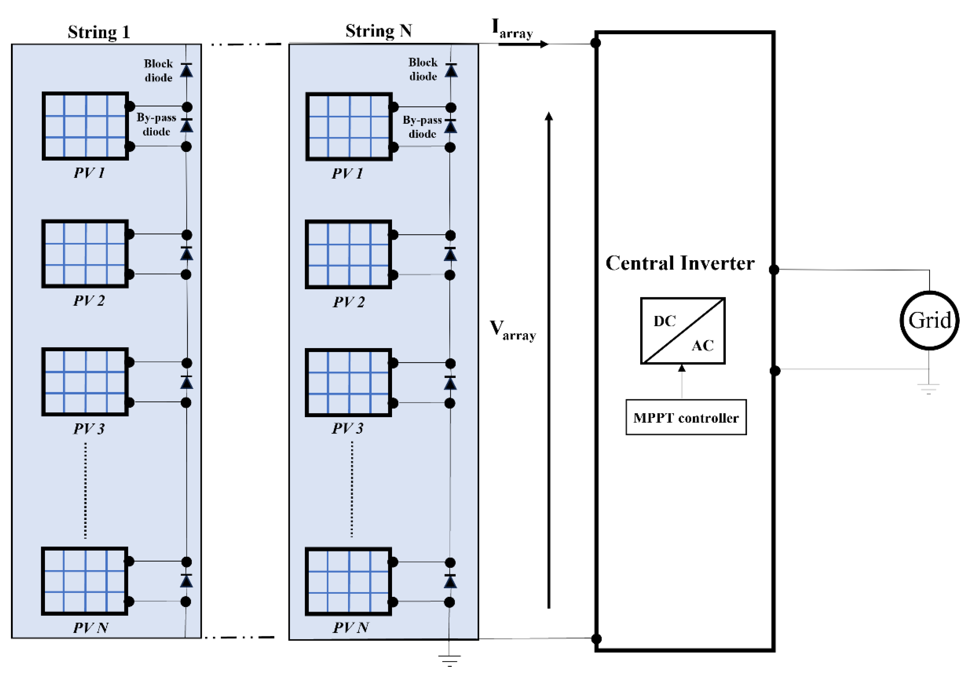
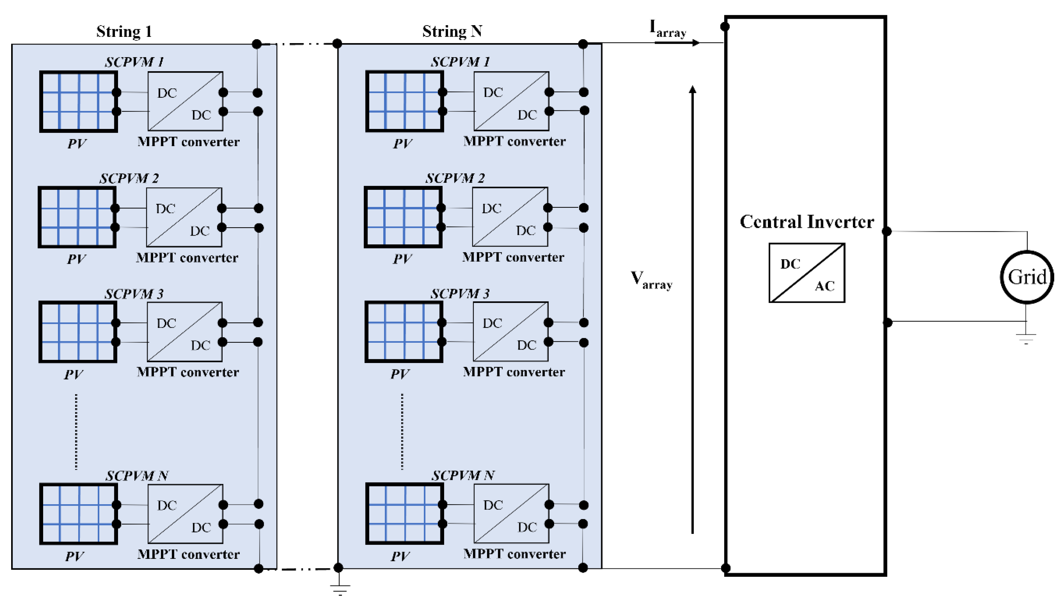
According to forecasts of the International Energy Agency (IEA), the world renewable capacity will increase by almost 2400 GW between 2022 and 2027; solar PV will represent over 60% of all renewable capacity expansion [1]. PV energy sources are the most attractive renewable sources, due to their availability and sustainability. Thanks to simpleness and modularity of installation, PV power plants of different sizes are now widespread all over the world. In a typical PV plant, modules are connected in series and create a string to provide the required output voltage; then, strings can be connected in parallel to form an array that can produce the required current. It is well known that, in the case of uniform temperature and irradiance conditions, the output current vs. voltage (I–V) characteristic of a PV array is non-linear and exhibits a unique Maximum Power Point (MPP) corresponding to the maximum power (PMPP) that the array is able to provide [2,3]. To ensure the maximum utilization of the array, it is essential to work in the MPP. Unfortunately, a direct connection of the output PV generator to the load (i.e., battery, AC grid, etc.) is not an optimal solution because in this case the operating point does not match with the MPP. In addition, the position of the MPP changes during the day due to many effects, such as changes in temperature and variation in solar radiation. For this reason, a Centralized Architecture (CA) of the PV array is adopted, where a central inverter, as shown in Figure 1, is generally interposed between the output terminals of the generator and the load; it must be able to change its parameters (i.e., its duty cycle) to adapt the load to the source to operate at MPP [4]. In such conditions, the energy performance is optimized [3] and the PV system behaves like a synchronized complex network, in which the extracted power is the maximum allowable and is the sum of the maximum power of each individual PV module [5,6]. A great variety of methods are able to track the MPP in PV plants; these so-called Maximum Power Point Tracking Techniques (MPPT) have been proposed in the literature and are categorized and commented on in many books and review papers [4,7,8,9,10,11].
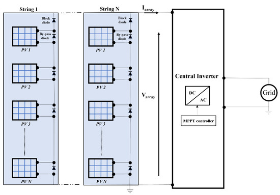
Figure 1.
A typical grid-connected CA scheme.
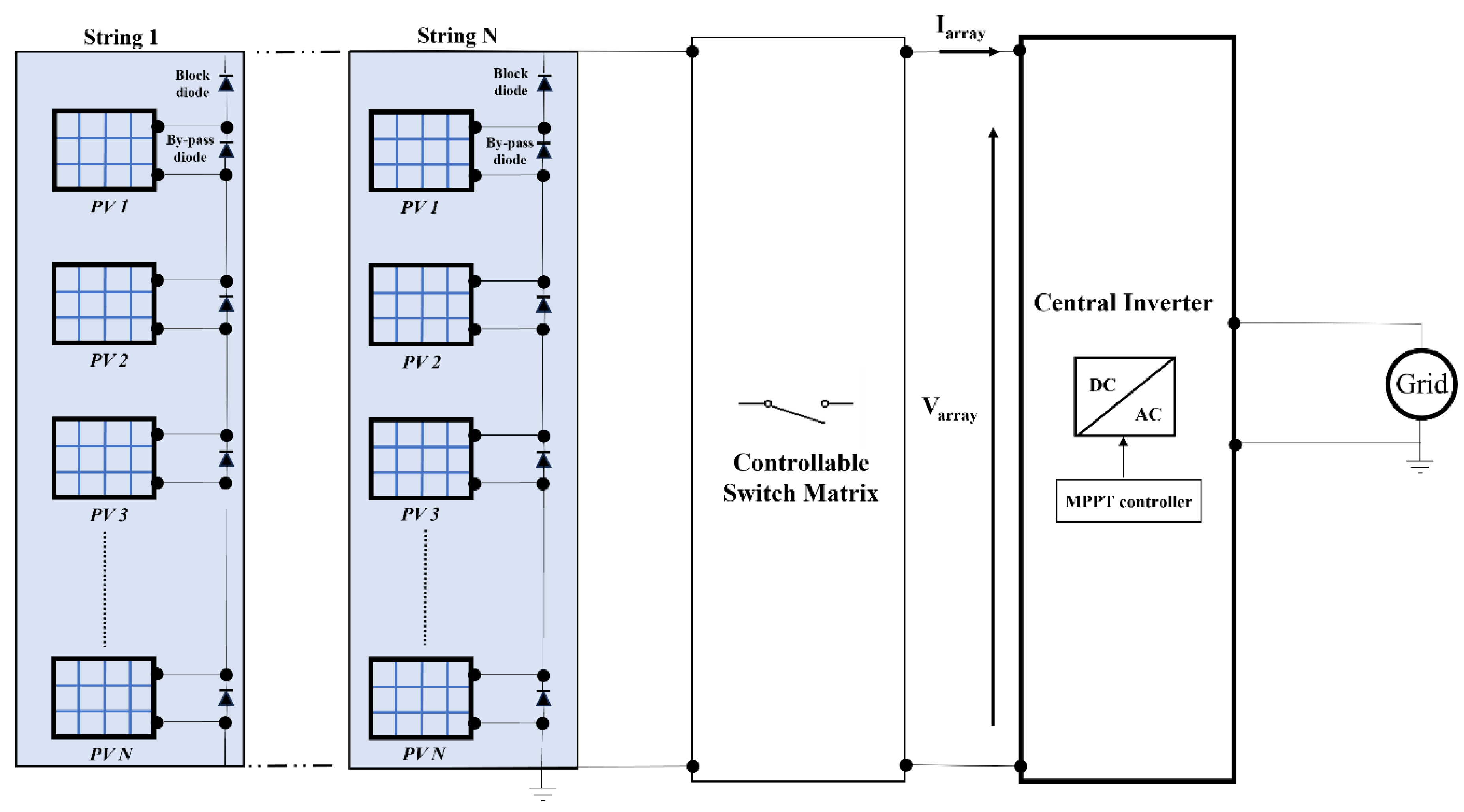
The classification includes the so-called “Hill Climbing”, “Curve Fitting”, “Dynamical” and “Machine Learning” MPPT techniques [10,12,13,14]. The above techniques are high-performing in the absence of mismatching operating conditions. Unfortunately, mismatching working conditions of the PV plant are very frequent. In such a case, the PV modules of an array operate in nonuniform conditions, due to shadowing of neighboring objects, dirtiness of modules, clouds, installation on irregular surfaces and different orientation angles of modules in the PV field, but also manufacturing tolerances or uneven aging, etc. In the case of mismatch, the PV modules are not synchronized and the maximum extractable power is lower than the sum of the maximum power over each individual PV module [15,16,17,18]. Moreover, the power vs. voltage (P–V) characteristic of the PV system may exhibit multiple peaks, one global maximum point (GMP) and many local peaks, due to the presence of bypass diodes used to protect PV modules from hot spots and thermal breakdown. Therefore, the efficiency of MPPT methods decreases dramatically [15,16,19]. For instance, the Perturb and Observe (P&O) technique, which is the most used method, may track local maxima, but not global maximum points [20] because they cannot differentiate the global maximum point with respect to local maxima. In conclusion, the impact and power loss due to mismatch depend on the PV modules’ operating points and on their electrical configuration. To maximize the efficiency of the module and track the global maximum point in case of mismatching conditions, a possible solution is offered by the dynamical reconfiguration of PV modules [21]. A basic scheme of a reconfigurable grid-connected PV system is shown in Figure 2. Like in complex networks, the topology of the network is dynamically changed using active switches to reach the synchronization of the modules and power maximization [22,23,24,25]. These techniques have proved to be efficient in mismatching conditions, although they are relatively expensive since they require the use of reliable devices able to switch high Direct Currents (DCs) [21,26,27]. An alternative solution to mitigate mismatching’s effects is the adoption of a Distributed Architecture (DA) in which, unlike the centralized one, each PV module, as shown in Figure 3, is equipped by an independent DC/DC converter and a dedicated Distributed Maximum Power Point Tracking (DMPPT) controller [28,29,30].
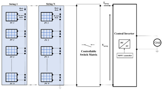
Figure 2.
Reconfigurable grid-connected scheme.
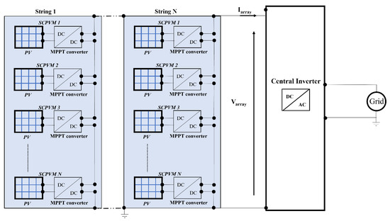
Figure 3.
DMPPT grid-connected scheme.
This kind of approach allows the negative effect of mismatched PV modules to be counteracted. Different architectures, based on Boost, Buck, Buck–Boost or Cuk topology, have been proposed for the resulting Self-Controlled PV Module (SCPVM) [31]. The main problem of this promising solution is the reliability of the DMPPT DC/DC converter. Moreover, the efficiency of the PV system is also related to a non-optimal value of the string voltage [32,33] and to the finite ratings of devices used in the power stage [31]. In a recent paper [34], some of the authors have theoretically shown that dynamical reconfiguration and Distributed Architecture are not alternative techniques but can be combined (combined approach) to get the maximum efficiency of the PV system. In particular, the authors showed, as a “proof of concept”, how in different mismatching scenarios, the critical issues affecting the distributed approach can be overcome by acting on the configuration of a PV array. However, no experimental tests have been described in that paper. The authors have also recently proposed a flexible DMPPT emulator able to reproduce the output (I–V) characteristics of a Boost-based [35] DMPPT system, not only at different irradiance levels but also as a function of the maximum voltage that can be applied across the drain and source terminals (VDsmax) of the adopted silicon devices under turn-off conditions. However, in the paper the emulator was adopted only to explore the performance of the Boost-based DMPPT approach. To overcome the limitations of the previous papers, the aim of the present work is to introduce a new algorithm suitable for Series-Parallel-Series Reconfiguration Boost-based DMPPT architecture and to prove its effectiveness in experimental tests performed by using the flexible emulator. After the introduction, the paper is structured as follows: Section 2 explores the necessity of the joint adoption of DMPPT and reconfiguration approaches; Section 3 introduces a fast Boost-based DMPPT reconfiguration algorithm, based on clustering analysis; Section 4 and Section 5 present the conducted experimental activity; and lastly, the conclusion of this work is drawn in Section 6.
2. The Necessity of the Joint Adoption of Boost-Based DMPPT and Reconfiguration Approaches
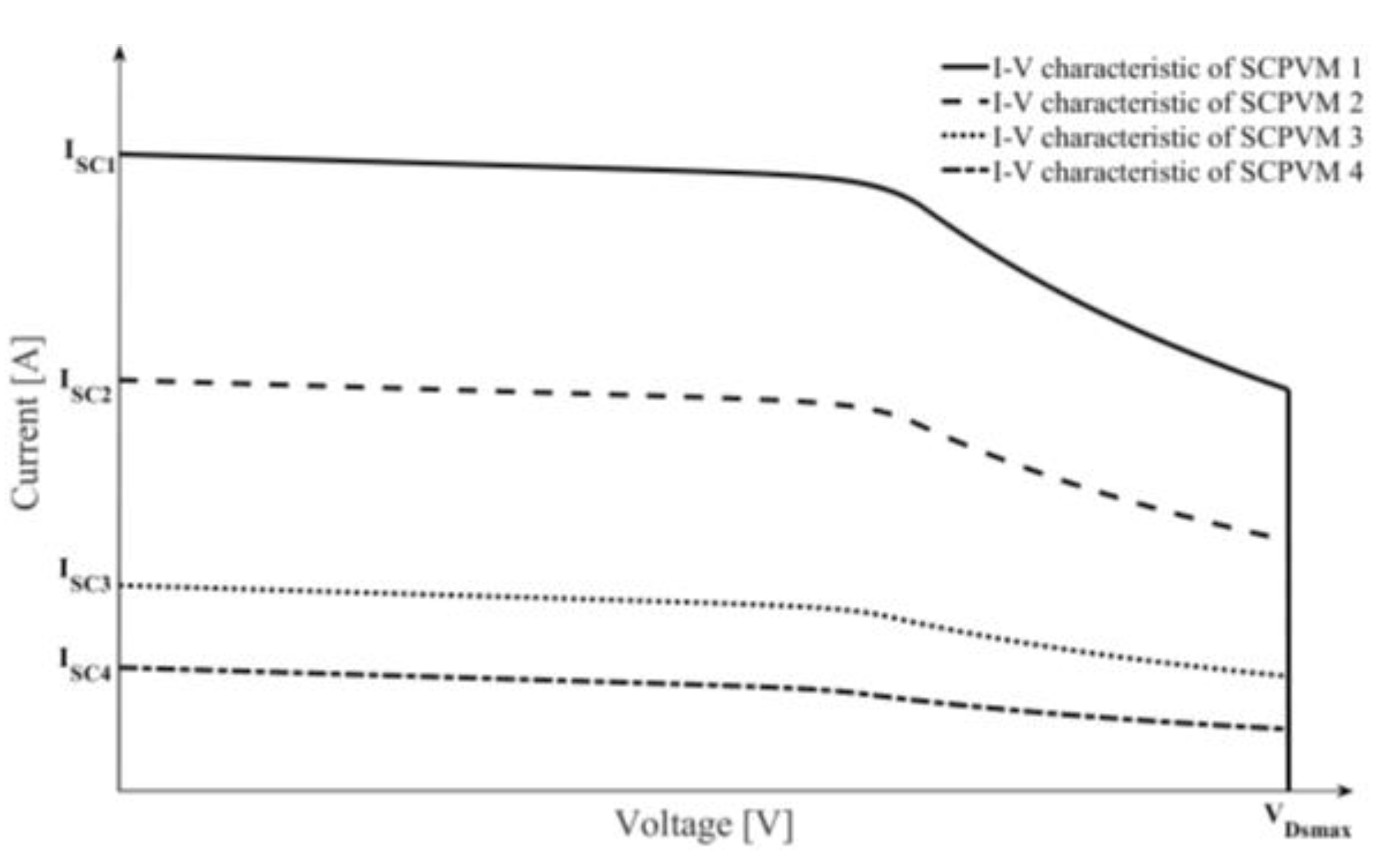
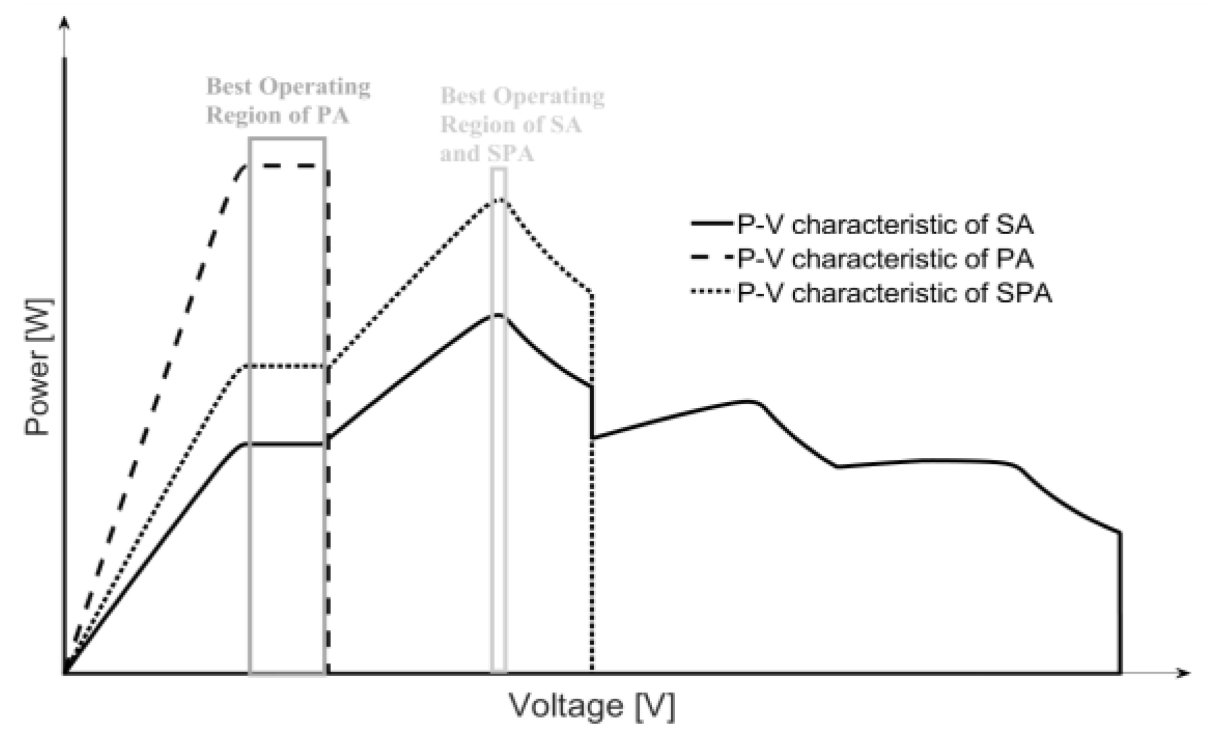
The reason why the Boost-based DMPPT approach alone is not able to effectively counteract the mismatching operating conditions is linked to the fact that its energetic performance is affected by the adopted electrical configuration (electrical connection between SCPVMs). To better clarify the above aspect, which directly leads to the proposed combined approach (joint adoption of Boost-based DMPPT and reconfiguration approaches), a simple PV system, composed by four Boost-based SCPVMs, will be used as a “case study”. With the aim to obtain results with general validity, no reference to numerical values, as shown in Figure 4 and Figure 5, will be made. The curves shown in Figure 4 represent the I–V characteristics of the SCPVMs that are considered mismatched. The mismatching scenario is characterized by the fact that all SCPVMs show different short circuit currents (ISC1, ISC2, ISC3 and ISC4), suggesting different operating irradiance values. The guidelines allowing the curves that are reported in Figure 4 to be obtained have been discussed in detail in Appendix A. Once the I–V characteristics of the considered SCPVMs are known, it is possible to easily obtain the P–V characteristic of whatever configuration. In our case study, the following three different architectures are compared: (I) Series Architecture (SA), (II) Parallel Architecture (PA) and (III) Series-Parallel Architecture (SPA). In particular, SA (PA) refers to a PV system composed of the series (parallel) connection of all SCPVMs and SPA refers to a string in which the parallel connection between SCPVM 1 and SCPVM 4 is connected in series with the parallel connection between SCPVM 2 and SCPVM 3. From Figure 5 it is evident that the shape of the P–V curves, and hence the amplitude and the position of the Best Operating Region (region in which the power extractable assumes its maximum value), are significantly influenced by means of the electrical connection between SCPVMs. This result suggests that, by acting on the configuration architecture with a controllable switch matrix, it is possible to increase the energetic performance of the mismatched Boost-based DMPPT PV systems.

Figure 4.
I–V characteristic of each SCPVM.
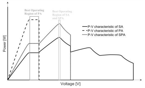
Figure 5.
P–V characteristic of each considered configurations.
3. Fast Series-Parallel-Series Reconfiguration Algorithm
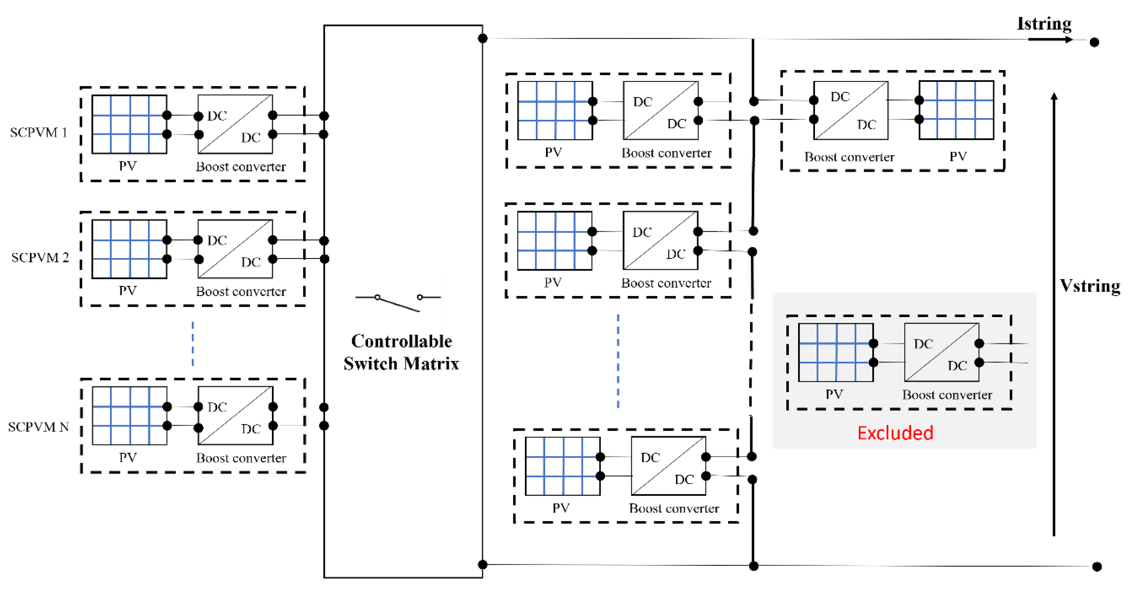
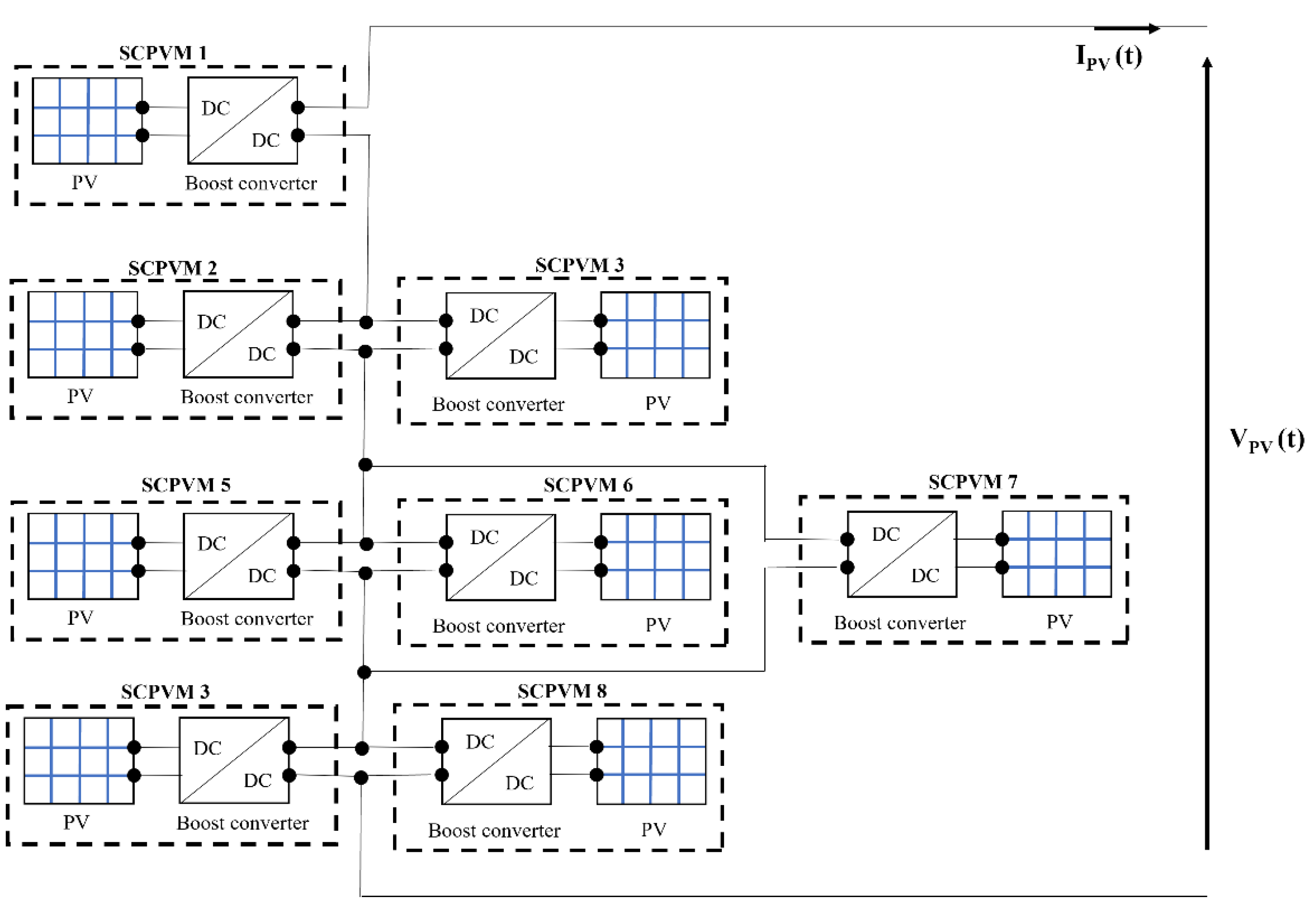
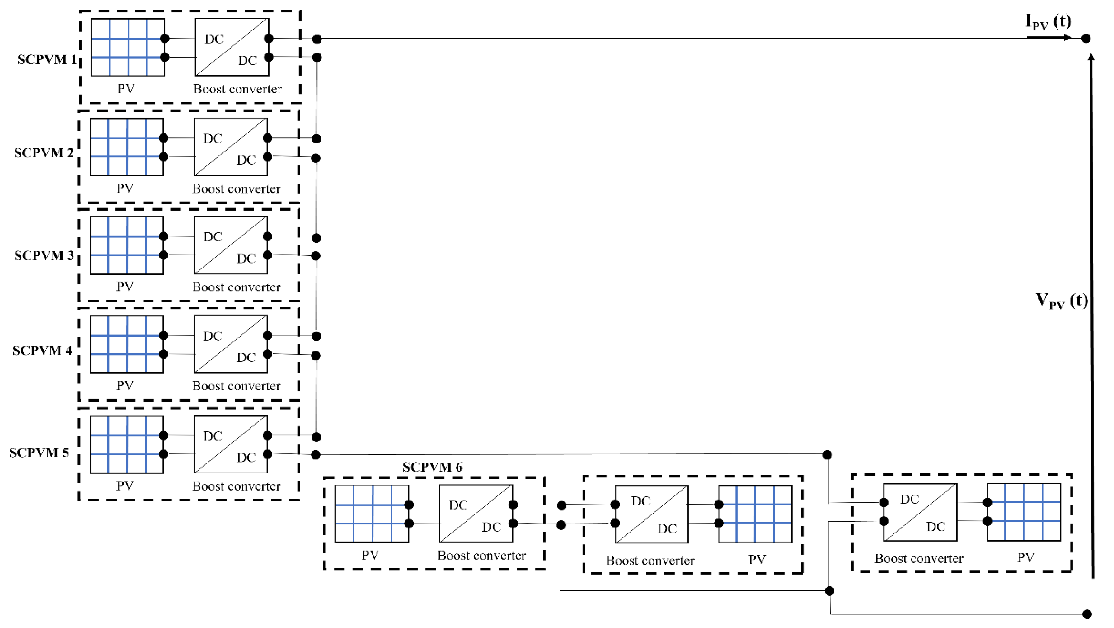
In the following, for the sake of simplicity, but without any loss of generality, a Boost-based DMPPT PV field made of N = 8 self-controlled PV modules will be considered. In Italy, most domestic PV plants are characterized by such architecture, with a power capability less than or equal to 3 kW. In addition, the monocrystalline solar panel capability of between 360 and 380 W represents, currently, an Italian market standard. As shown in Figure 6, the output of a proposed reconfiguration process, carried out with a proper controlled switch matrix, can be a Series-Parallel-Series (SPS) architecture in which several parallel clusters of SCPVMs are connected in series.
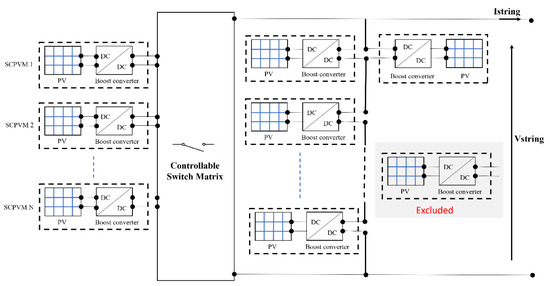
Figure 6.
Series-Parallel-Series reconfiguration DMPPT architecture.
In the considered network topology, in order to identify the configuration that represents the best compromise between efficiency and reliability, it will also be considered a possibility to exclude one or several SCPVMs; in particular, each SCPVM may belong to one of the identified series or parallel clusters or be disconnected. The only constraint, called string voltage constraint, is to ensure that the Optimal String Voltage Range (OSVR), which depends not only on the considered atmospheric conditions, in terms of irradiance and temperature values, but also on the topology [35], must exhibit an intersection (no-zero intersection) with the Optimal Working Range of the Inverter (OWRI). This means that the following condition must be satisfied:
where, OWRI is the voltage interval [Vmin, Vmax] between the minimum input voltage Vmin at which the inverter starts pulling power from the PV system and the maximum input voltage Vmax, that must never be exceeded to prevent damage to the inverter. Typical commercial values of, respectively, Vmin and Vmax are reported in Table 1.

Table 1.
Input voltage range of commercial PV inverters.
Based on the previous considerations, the proposed deterministic reconfiguration algorithm is made from the following three operating steps: (1) measurement; (2) identification of the optimal series configuration; (3) identification of the optimal SeriesPparallel-Series architecture.
Step 1 (Measurement step): The measurement step is voted to measure the short circuit current ISC,i of each SCPVM of the PV system. In fact, as shown in Appendix A, the knowledge of such current, together with the data obtained from the adopted PV module and Boost-based DC/DC converter’s datasheets, allows the determination of the approximate static I–V characteristic of the i-th SCPVM and, hence, the corresponding approximate Best Current (Voltage) Operating Range. In particular, once all the short circuit currents ISC,i (i = 1, 2, …, N) are known, the approximate i-th Best Operating Ranges are defined as follows:
where BCORi, and BVORi represent the i-th Best Current Operating Range and the i-th Best Voltage Operating Range, respectively. The meanings of β and VMPP_C are clarified in the Appendix section (Appendix A). Since the position and amplitude of such ranges are time-varying, depending on the atmospheric operating conditions, it is necessary to perform the measurement step periodically at fixed time intervals T∗. It is obvious that with higher f∗ = 1/T∗, there will also be a higher speed of variation in mismatching conditions which can be efficiently addressed by the proposed algorithm. On the other hand, the higher f∗ makes for a higher occurrence of short-circuit operating conditions in which the SCPVMs are not able to deliver power (higher waste of energy). In the following, for the sake of simplicity, the speed of tracking in the proposed algorithm will not be a subject of discussion. Our attention will be completely focused on the capability of the algorithm to identify the configuration that represents the best compromise between efficiency and reliability. In other words, an ideal lossless Boost DC/DC converter will be considered. Consequently, the efficiency of the Boost DC/DC converter will be assumed to be equal to one and the settling time will be argued as negligible (instantaneous system response). Step 1 ends with the creation of a list in which all SCPVMs are sorted in descending order, namely that the first SPCVM (SCPVM,1) has the highest irradiance value and, hence, the highest corresponding short-circuit current, while the N-th SCPVM (SCPVM,N) has the lowest short circuit current.
Step 2 (Identification of the optimal series configuration): The starting point of Step 2 is the construction of an intersection matrix (Im) that identifies the SCPVMs that can be connected in series to form efficient and reliable strings. The matrix Im is an [N × N] matrix, whose generic element Im(i,j) can take the value 0 or 1. The element Im(i,j) = 1 when i-th SCPVM and j-th SCPVM can be connected in series, that is, when the Best Current Operating Range of both SCPVMs have common values and Im(i,j) = 0 when the intersection between the Best Current Operating Range of both SCPVMs is an empty interval. The intersection matrix can, therefore, be defined as follows:
where i = 1, 2, …, N; and j = 1, 2, …, N.
Remembering that, after Step 1, all SCPVMs have been sorted in descending order, with decreasing irradiance values (ISC,i > ISC,j if (i > j)), the resulting matrix Im is an upper triangular sparse matrix, whose rows represent the set of all possible optimized series configuration clusters (CS,i with i = 1, 2, …, N). In particular, the generic i-th row of the intersection matrix identifies a reconfiguration architecture in which the maximum extractable power is equal to the sum of the maximum power that all the involved SCPVMs can provide in the considered atmospheric conditions (efficiency point of view). Of course, the identified series clusters are not exclusive because a single SCPVM may belong to one or more clusters. Then the generic i-th row identifies the number of SCPVMs that must be connected in series but also those who must be necessarily disconnected, to prevent one or more SCPVMs, belonging to i-th cluster (CS,i), from operating in the saturation state (reliability point of view). By denoting with jmax,i the maximum column index in which Im(i,jmax,i) = 1, the number of included (Nin,i) and excluded (Nex,i) SCPVMs for each CS,i are, respectively, as follows:
Once the N series configuration clusters have been identified, and the Maximum Series Cluster Extractable Power (MSCEPi) has been calculated for each of them, it is also necessary to evaluate the Optimal Series Cluster Voltage Range (OSCVRi) and the Optimal Series Cluster Current Range (OSCIRi), which are the optimal voltage (and current) range at which they have to operate in order to ensure optimal energetic performances. They can be calculated as [35] follows:
where i = 1, 2, …, N; and j = 1, 2, …, N.
In conclusion, the aim of Step 2 is to assemble a set of SCPVMs so that SCPVMs belonging to the same group, called a series configuration cluster, satisfy the first condition of Equation (4). In this way, N series configuration clusters can be identified, and the resulting matching strings are both efficient (the relative maximum extractable power is coincident with the relative maximum available power) and reliable (no SCPVM works in the saturation state). Another advantage of the above identification process is the low computational complexity since it is based on the definition of a triangular sparse matrix.
Step 3 (Identification of the optimal Series-Parallel-Series architecture): Step 3 is devoted to exploring, for all the N identified series configuration clusters, the possibility of also including the discarded Nex,i (with i = 1, 2,…, N) SCPVMs, while avoiding their operation in saturation state. Since the possibility of connecting each discarded panel in series with the selected cluster has already been evaluated and excluded from Step 2, a possible strategy involves the identification of the available Nex,i SCPVMs that can be connected in parallel with each other and then connected in series with the previous identified i-th series cluster. The obtained group of parallel panels is named parallel configuration cluster. To achieve this goal, Step 3 starts with the calculation of the total number NCP,i of parallel configuration clusters that can be associated to the i-th series configuration cluster:
Soon after, a cluster matrix (CLm,i) can be constructed, which identifies all the possible parallel clusters that can be associated with each series cluster. It is a [NCP, i × N] matrix defined as follows:
where k = 1, 2, …., NCl,i; and t = 1, 2, …, N.
The generic element is CLm,i(k,t) = 1 if the t-th SCPVM belongs to the k-th cluster, otherwise it is equal to zero. The cluster matrix is a sparse matrix since the number of non-zero elements for each row is between 2 and Nex,i, as the possibility of considering clusters with only one SCPVM has been already excluded in the previous steps (Steps 1 and 2) of the proposed algorithm. Moreover, for each row the minimum number of zero elements is Nin,i because they are related to the SCPVMs that belong to the i-th identified series configuration cluster that, obviously, cannot be included in the k-th parallel cluster. For the i-th series parallel cluster, it is definitely possible to determine Ncl,i parallel configuration clusters whose properties, in terms of Optimal Parallel Cluster Voltage Range (OPCVRi,k), Optimal Parallel Cluster Current Range (OPCIRi,k) and Maximum Parallel Cluster Extractable Power (MPCEPi,k), are obtained using the following equations:
At this point, the proposed algorithm is trained to restart Steps 1 and 2 by treating each identified parallel cluster as an equivalent SCPVM whose electrical characteristics are those obtained using Equations (12)–(14). Step 3 ends with the identification of the SPS configuration that exhibits the maximum extractable power included in the input inverter voltage range. In terms of computational complexity, the same considerations drawn for Step 2 also hold for Step 3. Both steps are based on the storage and manipulation of sparse matrices. Moreover, the ability to terminate the finding process in advance once the SPS architecture, in which all SCPVMs are electrically connected, has been identified, allows consideration of the proposed iterative algorithm, based on the binomial expansion, as a time-saving reconfiguration algorithm. The above statement is clearer if we compare the performance of the proposed algorithm with the commonly used stochastic reconfiguration algorithms, that, generally, employ a much higher number of trials to reach convergence.
4. Reconfigurable Series-Parallel-Series Emulator
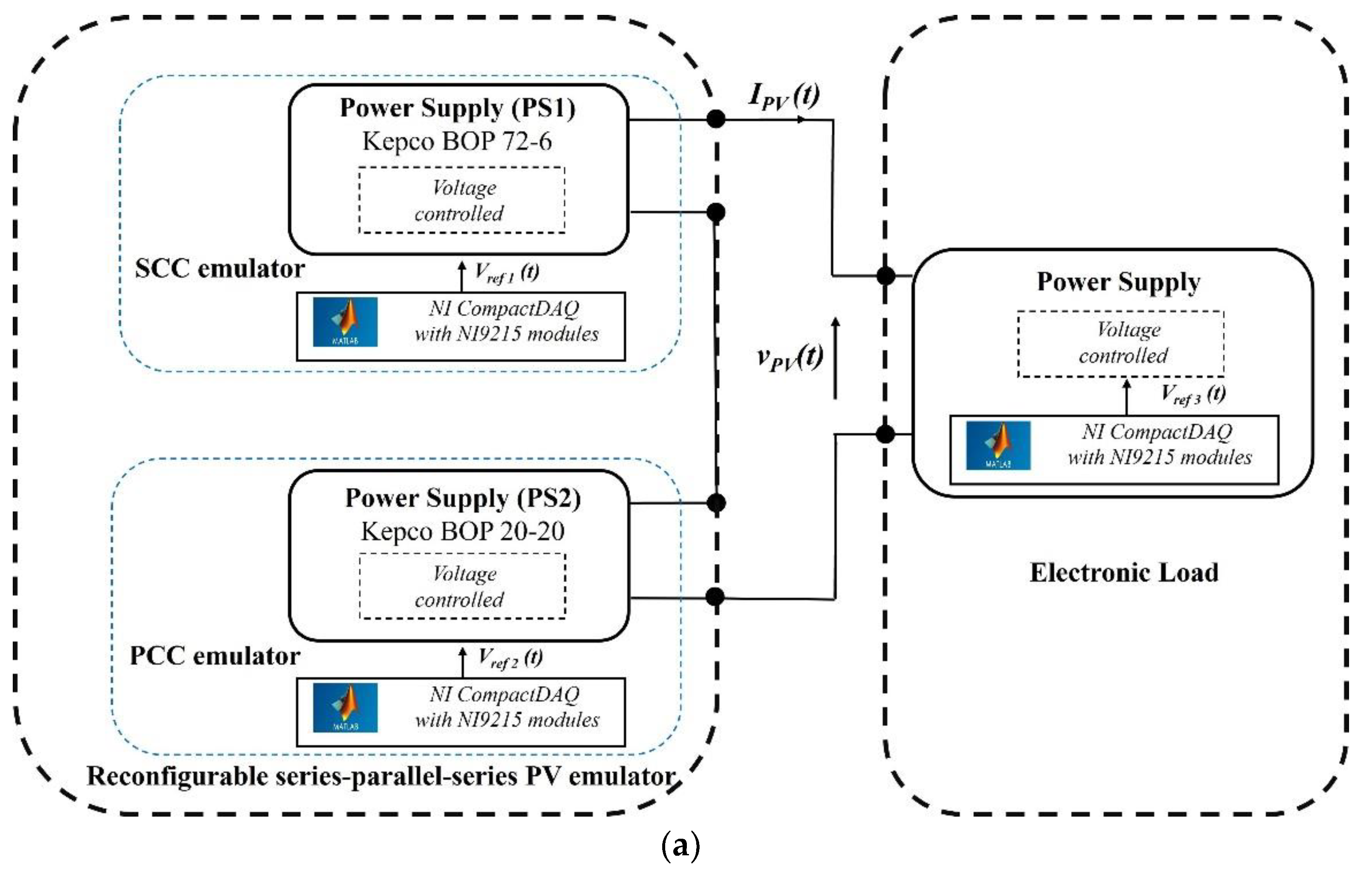
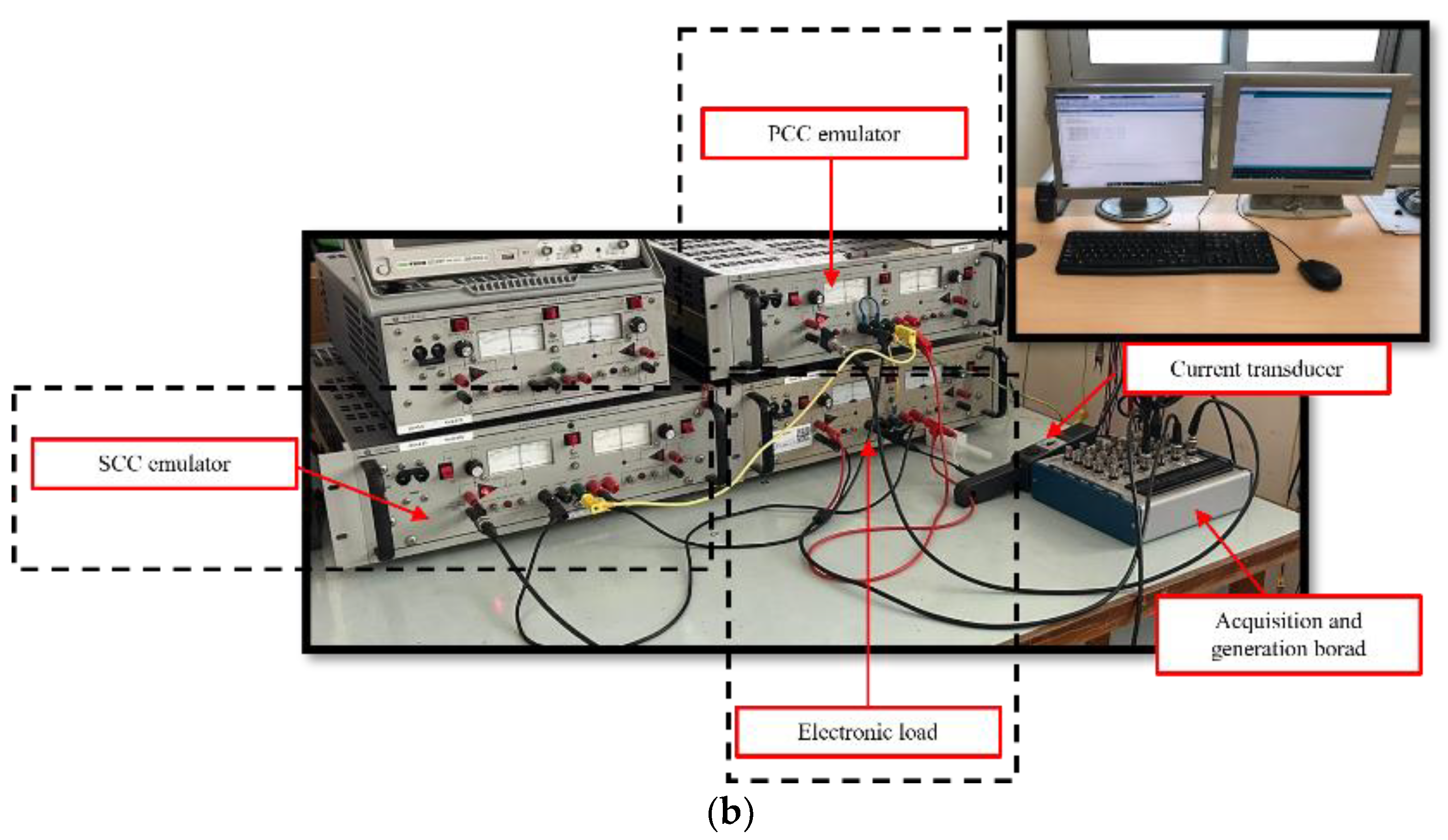
The proposed algorithm has been verified experimentally by the laboratory setup whose schematic and physical implementation are shown in Figure 7. The test bed consists of two fundamental blocks, i.e., the Emulation Block (EB) and the Acquisition and Generation Block (AGB). The emulation block is carried out by three commercial controlled power supplies (Kepco BOP). The first two (PS1 and PS2) being, respectively, the power stage of the Series Configuration Cluster (SCC) emulator and the Parallel Configuration Cluster (PCC) emulator. The third one is used as an “Electronic Load” to scan the I–V characteristics of the proposed Reconfigurable Series-Parallel-Series Emulator (RSPSE), featured by the series connection of the above two emulators (SCC emulator and PCC emulator). The three power supplies can work in all four quadrants of the current–voltage plane. They are linear power supplies with two bipolar control channels (voltage or current mode), selectable and individually controllable by either front panel controls or remote signals. The electrical characteristics of the overall system are reported in Table 2. It is evident that the proposed experimental setup is suitable for the emulation of reconfigurable domestic PV systems, characterized by severe mismatching scenarios.
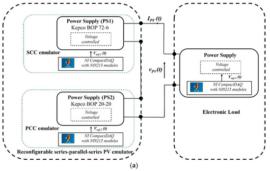

Figure 7.
Series-Parallel-Series reconfigurable domestic PV system setup: (a) block diagram; (b) experimental setup.
Table 2.
Electrical characteristics of the proposed RSPSE.
Moreover, the AGB consists of a modular National Instruments (Austin, TX, USA) USB system (NICompactDAQ 9174 with NI 9215 modules characterized by 16-bit resolution and a maximum sampling frequency of 100 kS/s) that allows backup and management of the experimental data in a MATLAB (R2022b) environment by MathWorks, Inc (Massachusetts, USA). Each input channel has its own analog to digital converter enabling the simultaneous recording of the PV voltage VPV(t) and the PV current IPV(t).
5. Experimental Results
In the following, the results obtained using the proposed algorithm will be considered with reference to two different mismatching scenarios: Case I and Case II. In both cases, the emulated PV system is characterized by the presence of N = 8 SCPVMs, whose electrical characteristics are listed in Table 3. As far as the electronic load is concerned, it will be assumed that it is characterized by an operating range whose values are shown in Table 4.
Table 3.
Electrical characteristics of the SCPVMs.
Table 4.
Input voltage range of the emulated inverter.
5.1. CASE I
Case I refers to the following ordered short circuit current vector, which can be obtained by applying Step 1 of the proposed algorithm: ISC_V = [2.04 1.13 0.92 0.82 0.7 0.7 0.7 0.7 0.5]A. The corresponding values of BCORs are listed in Table 5.
Table 5.
Best operating current ranges for Case I.
With reference to Case 1, the intersection matrix, obtained by applying the conditions expressed in (4), appears as follows:
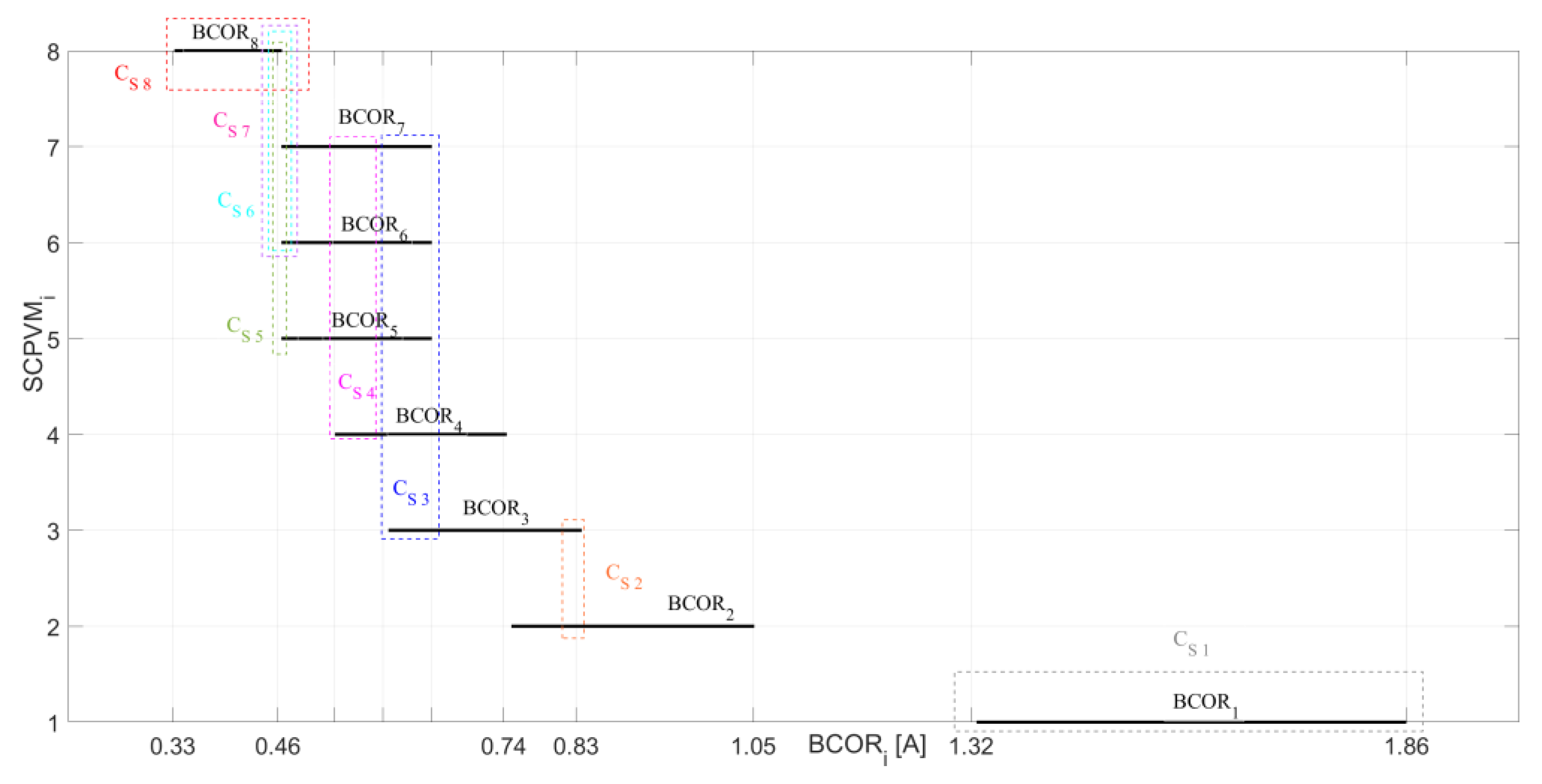
As shown before, each row of the identified intersection matrix represents a series configuration vector whose characteristics are reported in Table 6. As an example, cluster 6, represented at row 6 of the intersection matrix Im, is composed of panels SPVCM6, SPVCM7 and SPVCM8. The maximum extractable power from this cluster is MSCEP6 = 18.9069 W, the optimal series cluster voltage range is OSCVR6 = [40, 40-66, 714] V and the Nex,6 excluded panels are 5 and can be connected in NCP,6 = 26 possible parallel combinations. Figure 8 shows the obtained clusters and the corresponding optimal series voltage range.
Table 6.
Electrical characteristics of the identified CSs for Case I.
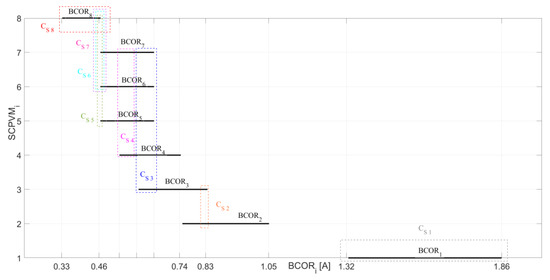
Figure 8.
BCORs and CSs of Case I.
Once the series configuration clusters are known, the proposed algorithm starts the identification of the corresponding parallel configuration clusters through a binomial expansion approach. The number of parallel configuration clusters that can be associated with the i-th series configuration is reported in the last column of Table 6. In the considered case, the investigation phase ends by analyzing the performances of SPS architectures built starting from the series configuration cluster C1, since the possibility of including all SCPVMs, as shown in Figure 9, belongs to the above group.
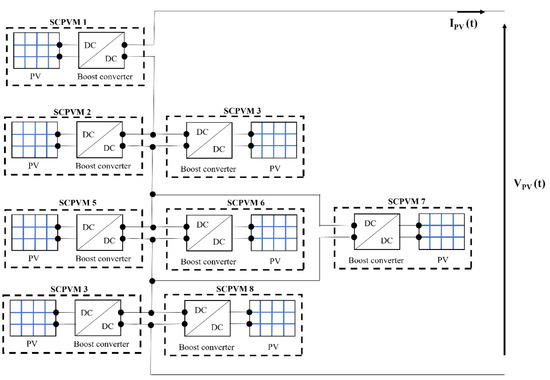
Figure 9.
The identified SPS architecture for Case I.
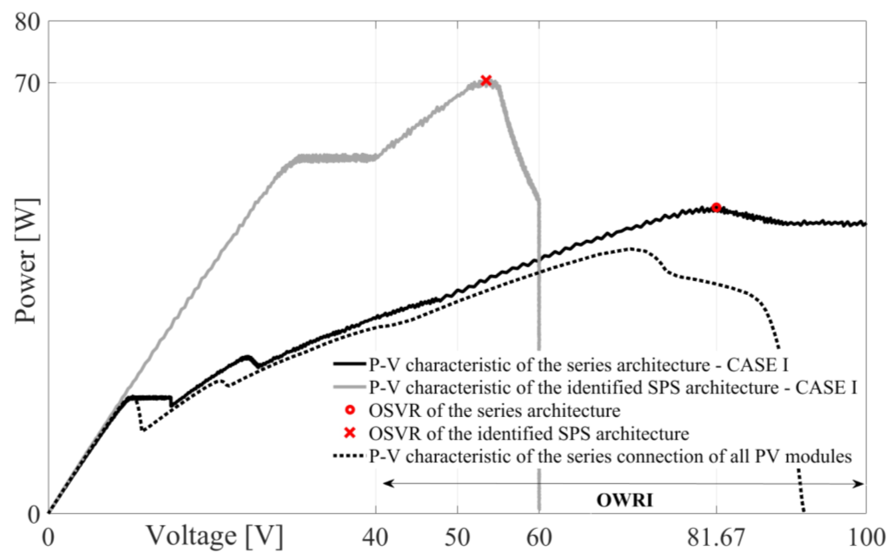
In conclusion, to further highlight the results obtained using the proposed algorithm, Figure 10 compares the P–V characteristics of the string just identified (grey line) with that obtained by using the “classical approach”, that is, connecting in series all the eight SCPVMs (black line).
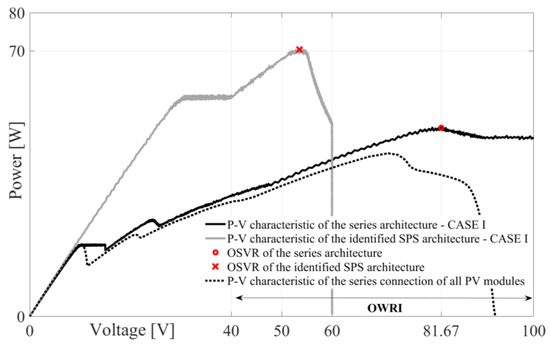
Figure 10.
P–V characteristics of the series and the identified SPS architectures (Case I).
From Figure 10 it is evident that there is a sensible increase in the extractable power in the operating range of the inverter, estimated as ~41%; a percentage that may exceed 60% in comparison with the performance of the CA architecture (dot curve of Figure 10), in which all PV modules are connected in series.
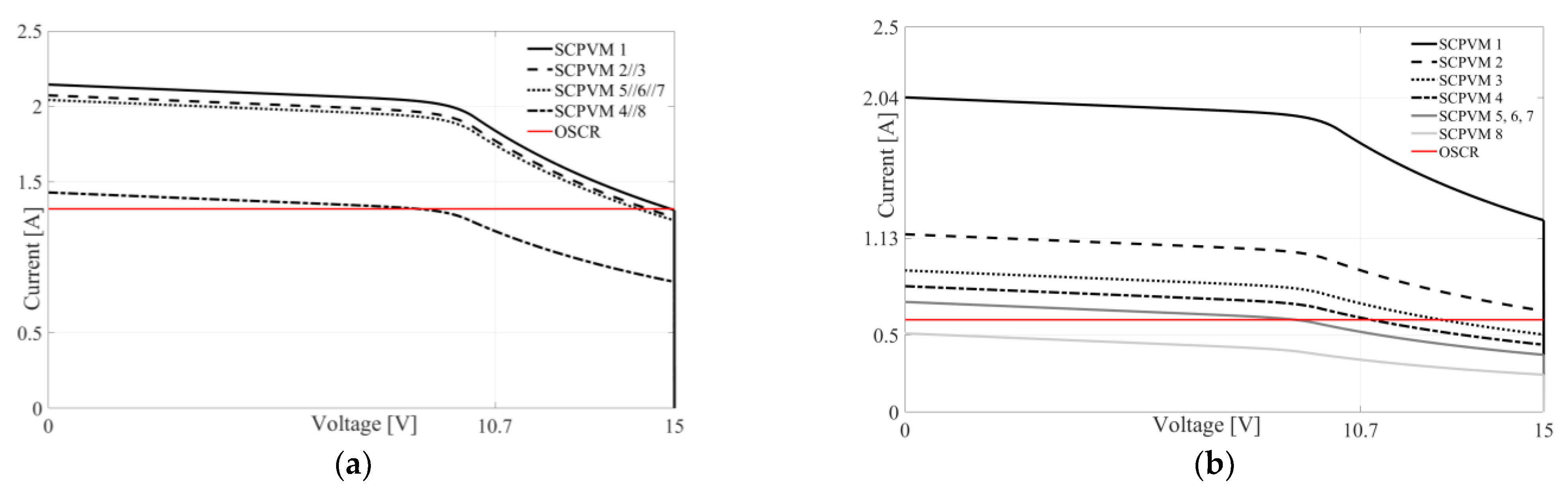
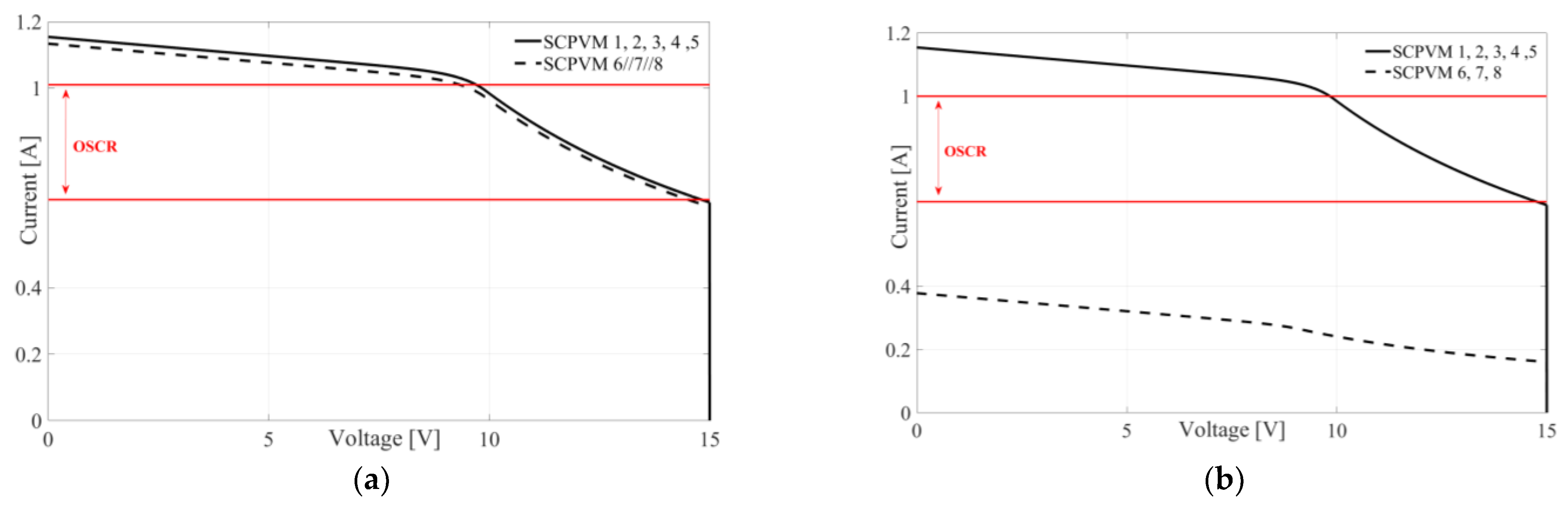
The increased extractable power is not the only advantage of using the proposed approach. Referring to the identified SPS architecture (Figure 11a), the saturation and reverse bias working conditions are completely avoided, since in the Optimal String Current Range (OSCR), that in this case collapses at one point, all SCPVMs can provide the maximum available power. The same considerations do not hold for the standard series architecture, since the OSCR (red curve of Figure 11b) does not intersect the branches of the hyperbole of all SCPVMs. The SCPVM1, SCPVM2 and SCPVM8 are excluded. In particular, the first two work in the saturation state, while SCPVM8 works in a reverse bias condition since the OSCR is higher than its short circuit current. In conclusion, in the identified SPS architecture, the negative effects of mismatching conditions are completely mitigated.
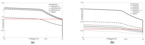
Figure 11.
I–V characteristics of each series and parallel configuration clusters (a) and each SCPVM (b) Case I.
5.2. CASE II
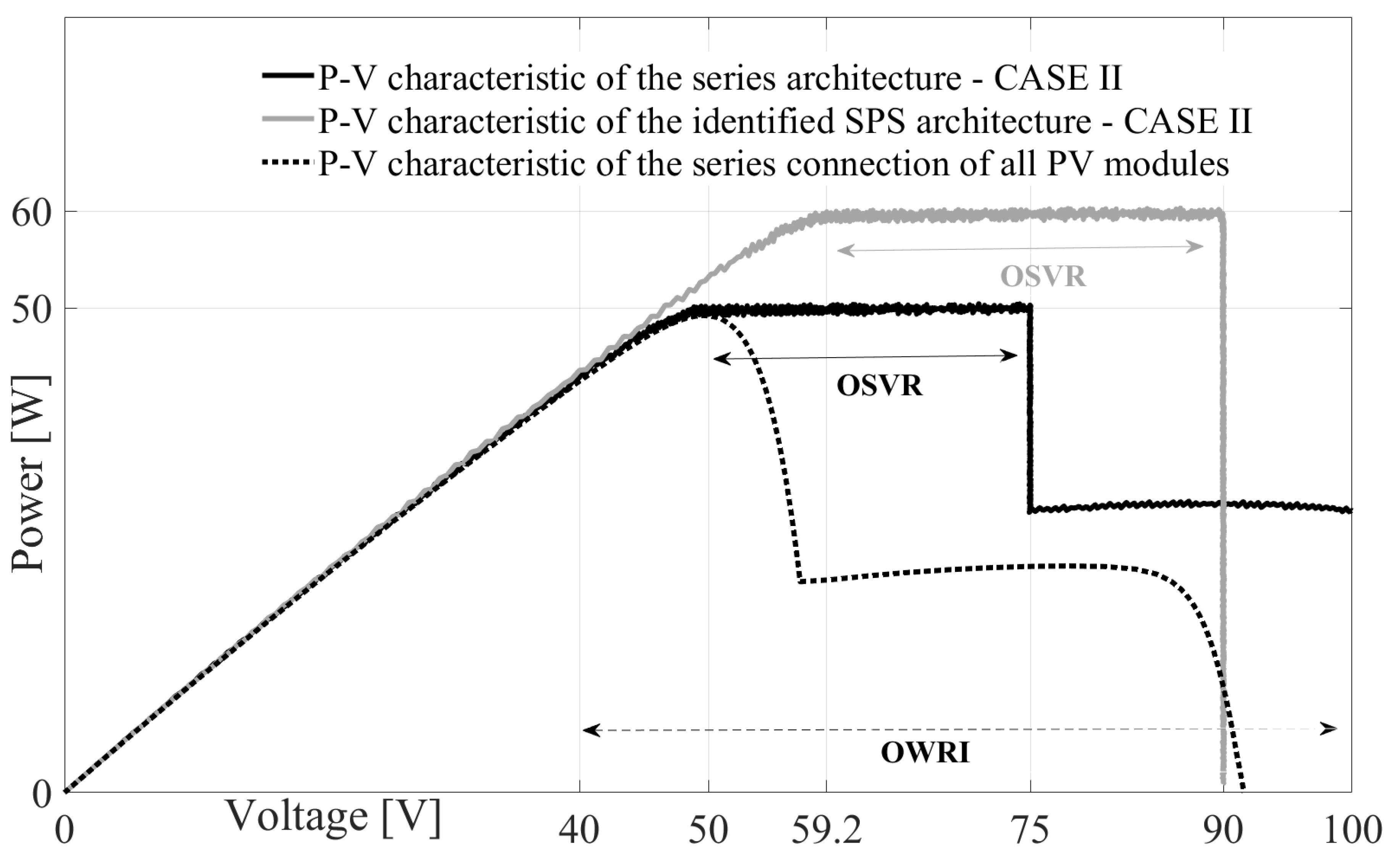
Case II refers to the following short circuit current vector: ISC_V = [1.13 1.13 1.13 1.13 1.13 0.37 0.37 0.37]A. Repeating the same steps previously illustrated led to the SPS architecture shown in Figure 12, and whose energetic performances are reported in Figure 13 and Figure 14. Even in this second considered case, the operating performance of the identified SPS architecture is higher than that obtained with the classical approaches, both in terms of efficiency (20% increase in extracted power) and reliability (no SCPVM works in the reverse and/or in the saturation state). On this last point, it is evident that, in the OSCR of the classical architecture (Figure 14b) the SCPVM6, SCPVM7 and SCPVM8 work in reverse bias conditions with consequent reduction of the reliability of the whole system. Even in this considered case, the proposed reconfiguration algorithm is able to face the efficiency and reliability reduction when mismatching conditions occur.

Figure 12.
The identified SPS architecture for Case II.
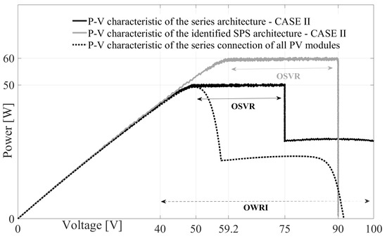
Figure 13.
P–V characteristics of the series and the identified SPS architectures (Case II).
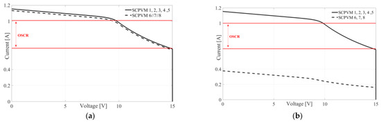
Figure 14.
I–V characteristics of each series and parallel configuration clusters (a) and each SCPVM (b) Case II.
6. Conclusions
The aim of this work is to prove that the combined action of DMPPT and reconfiguration approaches represents a promising solution to maximize the energetic performances of PV systems in any mismatching operating conditions. For this purpose, a new algorithm, based on the complementary action of the DMPPT and reconfiguration approaches, has been proposed. Such an algorithm is based on the periodic measurement of the short circuit currents of all PV modules. The considered topology is the reconfigurable Series-Parallel-Series that is suitable for domestic PV application. The experimental results fully confirm the effectiveness of the proposed technique and provide evidence of its major advantages: robustness, simplicity of implementation and time-saving. The main disadvantage of the proposed algorithm is the waste of energy during the measurement step in which the PV system works in the short circuit condition. Further work is in progress to extend the above approach, not only to more complex topologies, but also to more severe mismatching operating conditions in which the measurement time step negatively affects the performance of the whole PV system.
Author Contributions
Conceptualization, M.B. (Marco Balato) and C.P.; methodology, M.B. (Marco Balato) and C.P.; software, M.B. (Marco Balato), C.P. and A.L.; validation, M.B. (Marco Balato), C.P. and A.L.; formal analysis, M.B. (Marco Balato), C.P. and A.L.; investigation, M.B. (Marco Balato), C.P., A.L., M.B. (Martina Botti) and L.V.; resources, M.B. (Marco Balato), C.P. and A.L.; data curation, M.B. (Marco Balato), C.P. and A.L.; writing—original draft preparation, M.B. (Marco Balato) and C.P.; writing—review and editing, M.B. (Marco Balato), C.P., A.L., M.B. (Martina Botti) and L.V.; visualization, M.B. (Marco Balato), C.P. and A.L. All authors have read and agreed to the published version of the manuscript.
Funding
This research received no external funding.
Data Availability Statement
No new data were created or analyzed in this study. Data sharing is not applicable to this article.
Conflicts of Interest
The authors declare no conflict of interest.
Appendix A. The Exact and Approximate I–V and P–V Characteristics of a Single Boost-Based SCPVM
A few simple tools to obtain the current vs. voltage (I–VI–V) and the power vs. voltage output static characteristics of a lossless Boost-based SCPVM are provided. The knowledge of such properties represents the starting point to the development of the I–V and P–V characteristics of an SPS architecture, in which several PCs of SCPVMs are connected in series. To this aim, the system shown in Figure A1, which consists of a PV module equipped with its own Boost DC/DC converter, implementing the DMPPT function, will be considered and analyzed.
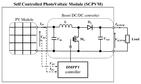
Figure A1.
Circuit model of Boost-based SCPVM.
Figure A1.
Circuit model of Boost-based SCPVM.
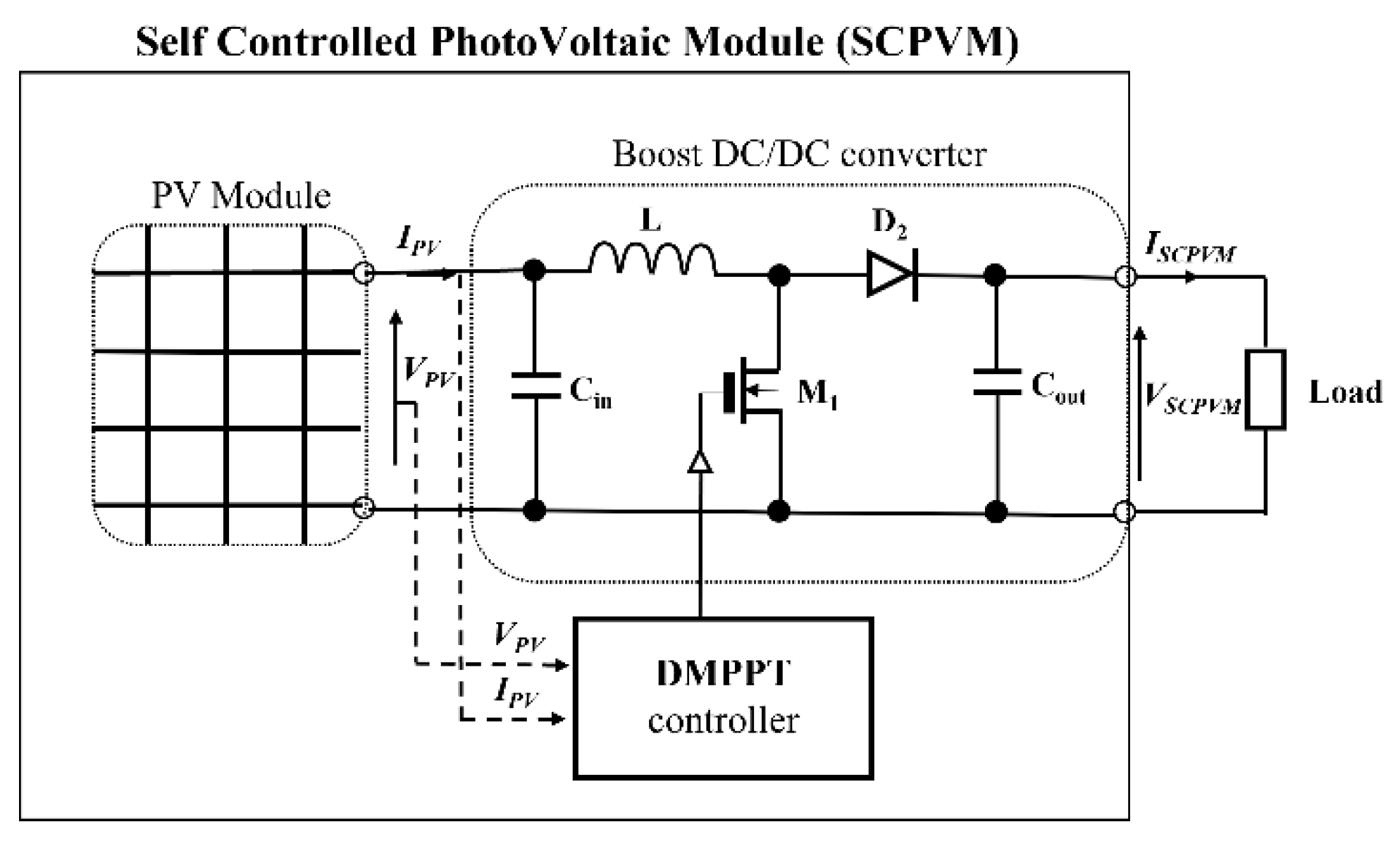
In the above figure, IPV (VPV) and ISCPVM (VSCPVM) denote currents (voltages) at the input and output ports of the Boost DC/DC converter, respectively. Moreover, the symbol PPV (PSCPVM) indicates the power extracted from the PV module (SCPVM). In Figure A2, the typical output static I–V characteristics of a PV module (black line) and of a SCPVM (dashed line) are reported, at constant irradiance (S) and temperature (T) values. It is assumed that the losses occurring in the power stage of the Boost converter (switching, conduction and iron losses) and the settling time of the step response of a closed or open loop SCPVM are neglected. In addition, the MPPT efficiency of the DMPPT controller is assumed equal to one (ηDMPPT = 1). In this scenario, the output I–V characteristic of a single SCPVM is characterized by the presence of a Best Operating Region (BOR) bounded by two ranges: voltage (BVOR) and current (BCOR) ranges [35]. The above ranges are set out as follows:
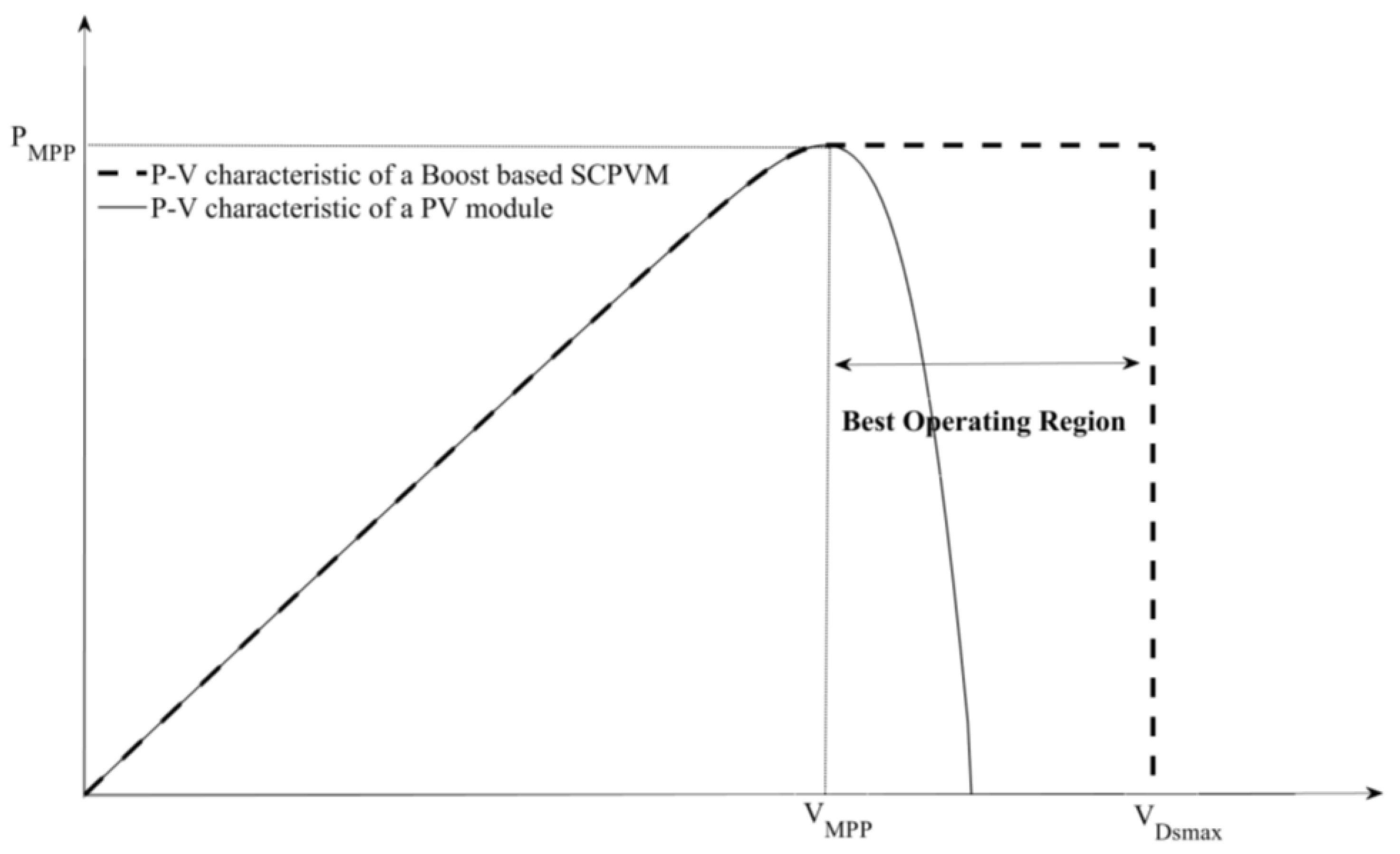
where VDSmax is the maximal allowed voltage provided by the utilized silicon devices and PMPP (VMPP) is the maximum power (voltage) that can be provided by the adopted PV module under the considered atmospheric conditions (irradiance and ambient temperature) [35]. From the I–V characteristic, it is then easy to obtain the corresponding power vs. voltage (P–V) characteristic. An example of P–V characteristic of a single Boost-based SCPVM is shown in Figure A3.
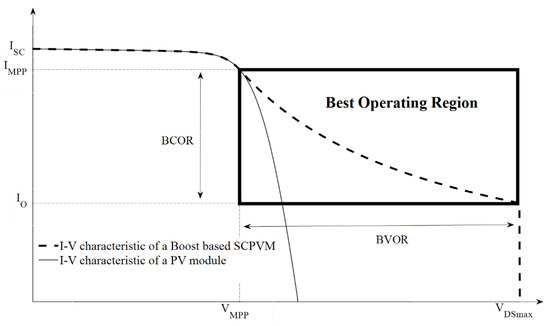
Figure A2.
PV module and Boost-based SCPVM I–V characteristics.
Figure A2.
PV module and Boost-based SCPVM I–V characteristics.
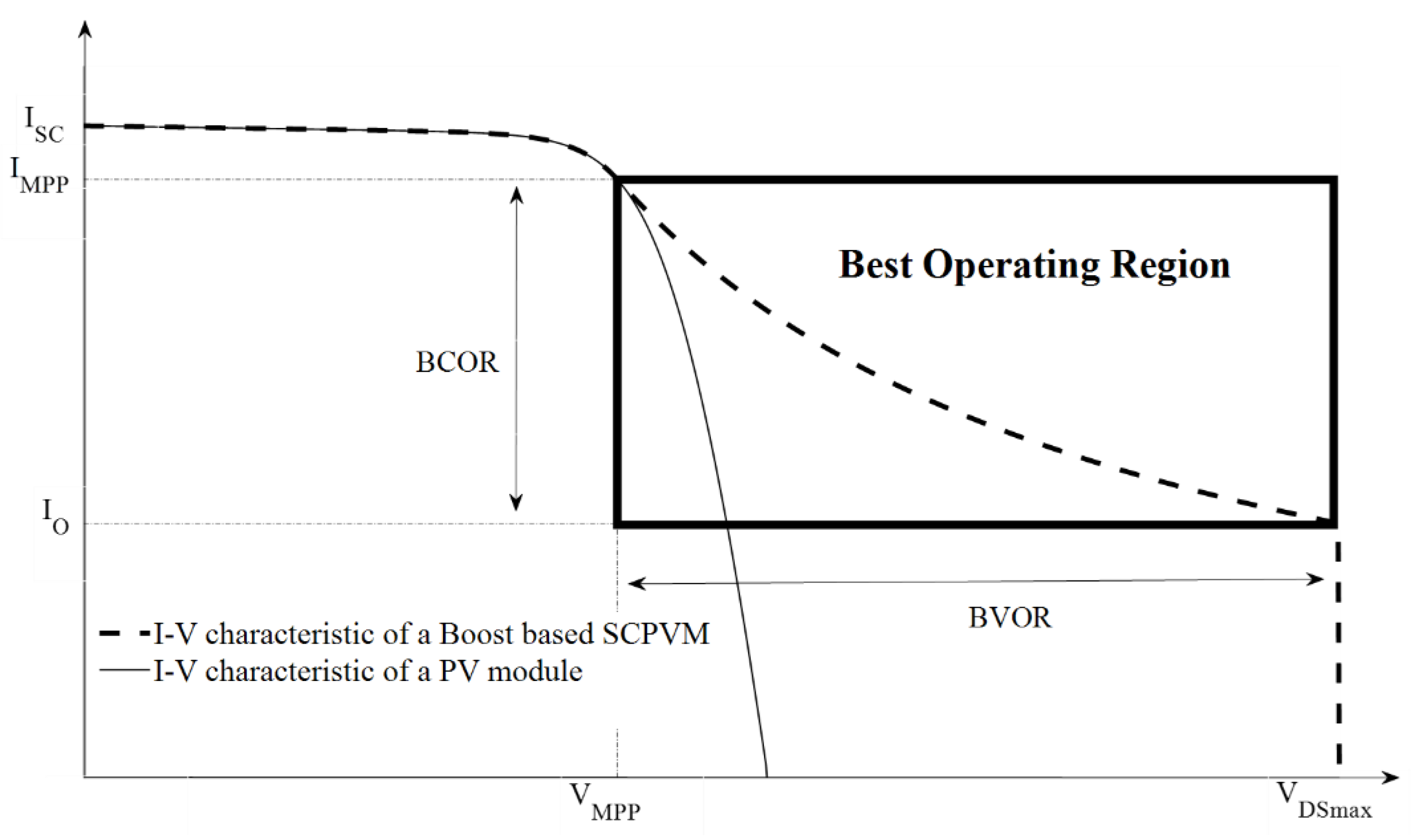

Figure A3.
PV module and Boost-based SCPVM P–V characteristics.
Figure A3.
PV module and Boost-based SCPVM P–V characteristics.
To get enough accurate information concerning BOR, it is not necessary to deal with the exact I–V characteristic of a single Boost-based SCPVM, but a proper approximate version of such a characteristic is enough. The approximated I–V SCPVM characteristic is obtained by considering two hypotheses. The first one is to consider the Maximum Power Point Voltage (VMPP) constant (VMPP_C) instead of varying with time. In particular, the following will be imposed:
where VMPP_C represents the VMPP in Standard Operating Conditions (STC). The easy availability of VMPP_C on the manufacturers’ datasheets is the main advantage of this approach. The second hypothesis is based on the substitution of that part of the I–V characteristic for VSCPVM ≤ VMPP, which cannot be expressed in an easy explicit form I = f(V) [35], with a simpler constant characteristic:
where β is the ratio between IMPP_STC (MPP current in STC) and IMPP_STC (short circuit current in STC). Typically, it is β = 0.93, a value that will be used in the following discussion. This approximation can be justified by considering that the exact I–V characteristic is more or less flat, for VSCPVM ≤ VMPP. The hyperbolic equation that characterizes the approximate BOR is, of course, PSCPVM = VMPP_C β ISC. It is worth noting that other, more accurate, forms of approximation of the curve for VSCPVM ≤ VMPP might be, in principle, used; for example, a piece-wise linear approximation. But, as it has been shown in [35], it is not necessary at all. In fact, the use of the simple approximation ISCPVM = β ISC for VSCPVM ≤ VMPP and PSCPVM = VMPP_C β ISC for VMPP ≤ VSCPVM ≤ VDSmax, allows the calculations needed by the proposed technique for a proper reconfiguration of all SCPVMs to be easily carried out in closed form, with enough accuracy. The above discussion is summarized in Figure A4, in which the comparison between the exact (solid line) and approximate (dashed line) versions of the I–V characteristic of a single Boost-based DC/DC converter are reported.
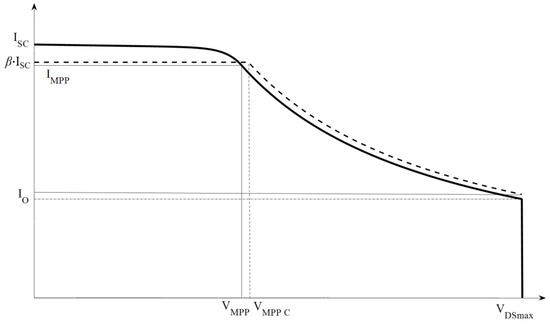
Figure A4.
Exact (solid line) and approximate (dashed line) I–V characteristics of a single Boost-based SCPVM.
Figure A4.
Exact (solid line) and approximate (dashed line) I–V characteristics of a single Boost-based SCPVM.

References
- Renewables. Analysis and Forecast to 2022; Technical Report; International Energy Agency: Paris, France, 2023.
- Femia, N.; Petrone, G.; Spagnuolo, G.; Vitelli, M. Power Electronics and Control Techniques for Maximum Energy Harvesting in Photovoltaic Systems; CRC Press, Taylor and Francis Group: Boca Raton, FL, USA, 2012. [Google Scholar]
- Eltamaly, A.M.; Abdelaziz, A.Y. Modern Maximum Power Point Tracking Techniques for Photovoltaic Energy Systems; Springer: Berlin/Heidelberg, Germany, 2020. [Google Scholar]
- Liu, H.; Khan, M.Y.A.; Yuan, X. Hybrid Maximum Power Extraction Methods for Photovoltaic Systems: A Comprehensive Review. Energies 2023, 16, 5665. [Google Scholar] [CrossRef]
- Pikovsky, A.; Rosenblum, M.; Kurths, J. Synchronization. In A Universal Concept in Nonlinear Sciences; Cambridge University Press: Cambridge, UK, 2001. [Google Scholar]
- Burbano-L, D.A.; Yaghouti, S.; Petrarca, C.; de Magistris, M.; di Bernardo, M. Synchronization in Multiplex Networks of Chua’s Circuits: Theory and Experiments. IEEE Trans. Circuits Syst. I Regul. Pap. 2020, 67, 927–938. [Google Scholar] [CrossRef]
- Sarvi, M.; Azadian, A. A comprehensive review and classified comparison of MPPT algorithms in PV systems. Energy Syst. 2022, 13, 281–320. [Google Scholar] [CrossRef]
- Derbeli, M.; Napole, C.; Barambones, O.; Sanchez, J.; Calvo, I.; Fernández-Bustamante, P. Maximum Power Point Tracking Techniques for Photovoltaic Panel: A Review and Experimental Applications. Energies 2021, 14, 7806. [Google Scholar] [CrossRef]
- Yap, K.Y.; Sarimuthu, C.R.; Lim, J.M.Y. Artificial Intelligence Based MPPT Techniques for Solar Power System: A review. J. Mod. Power Syst. Clean Energy 2020, 8, 1043–1059. [Google Scholar] [CrossRef]
- Motahhir, S.; El Hammoumi, A.; Ghzizal, A. The most used MPPT algorithms: Review and the suitable low-cost embedded board for each algorithm. J. Clean. Prod. 2020, 246, 118983. [Google Scholar] [CrossRef]
- Kabalci, E. Maximum Power Point Tracking (MPPT) Algorithms for Photovoltaic Systems. In Energy Harvesting and Energy Efficiency; Lecture Notes in Energy; Springer: Berlin/Heidelberg, Germany, 2017. [Google Scholar]
- Kottas, T.; Boutalis, Y.; Karlis, A. New maximum power point tracker for PV arrays using fuzzy controller in close cooperation with fuzzy cognitive networks. IEEE Trans. Energy Convers. 2006, 21, 793–803. [Google Scholar] [CrossRef]
- Daraban, S.; Petreus, D.; Morel, C. A novel MPPT (maximum power point tracking) algorithm based on a modified genetic algorithm specialized on tracking the global maximum power point in photovoltaic systems affected by partial shading. Energy 2014, 74, 374–388. [Google Scholar] [CrossRef]
- Bahgat, A.; Helwa, N.; Ahmad, G.; El Shenawy, E. Maximum power point traking controller for PV systems using neural networks. Renew. Energy 2005, 30, 1257–1268. [Google Scholar] [CrossRef]
- Al-hasan, A.; Ghoneim, A. A new correlation between photovoltaic panel’s efficiency and amount of sand dust accumulated on their surface. Int. J. Sustain. Energy 2005, 24, 187–197. [Google Scholar] [CrossRef]
- Silvestre, S.; Chouder, A. Effects of shadowing on photovoltaic module performance. Prog. Photovolt. 2008, 16, 141–149. [Google Scholar] [CrossRef]
- Adinoyi, M.J.; Said, S. Effect of dust accumulation on the power outputs of solar photovoltaic modules. Renew. Energy 2013, 60, 633–636. [Google Scholar] [CrossRef]
- Hussein, H.; Ahmad, G.; El-Ghetany, H. Performance evaluation of photovoltaic modules at different tilt angles and orientations. Energy Convers. Manag. 2004, 45, 2441–2452. [Google Scholar] [CrossRef]
- Romero-Cadaval, E.; Spagnuolo, G.; Franquelo, L.G.; Ramos-Paja, C.A.; Suntio, T.; Xiao, W.M. Grid-connected photovoltaic generation plants: Components and operation. IEEE Ind. Electron. Mag. 2013, 7, 6–20. [Google Scholar] [CrossRef]
- Ishaque, K.; Salam, Z.; Lauss, G. The performance of perturb and observe and incremental conductance maximum power point tracking method under dynamic weather conditions. Appl. Energy 2014, 119, 228–236. [Google Scholar] [CrossRef]
- Sai Krishna, G.; Moger, T. Reconfiguration strategies for reducing partial shading effects in photovoltaic arrays: State of the art. Sol. Energy 2019, 182, 429–452. [Google Scholar] [CrossRef]
- Ram, J.P.; Pillai, D.S.; Jang, Y.-E.; Kim, Y.-J. Reconfigured Photovoltaic Model to Facilitate Maximum Power Point Tracking for Micro and Nano-Grid Systems. Energies 2022, 15, 8860. [Google Scholar] [CrossRef]
- Bonthagorla, P.; Mikkili, S. Performance analysis of PV array configurations (SP, BL, HC and TT) to enhance maximum power under non-uniform shading conditions. Eng. Rep. 2020, 2, e12214. [Google Scholar] [CrossRef]
- de Magistris, M.; di Bernardo, M.; Manfredi, S.; Petrarca, C.; Yaghouti, S. Modular experimental setup for real-time analysis of emergent behavior in networks of Chua’s circuits. Int. J. Circuit Theory Appl. 2016, 44, 1551–1571. [Google Scholar] [CrossRef]
- Prince Winston, D.; Kumaravel, S.; Praveen Kumar, B.; Devakirubakaran, S. Performance improvement of solar PV array topologies during various partial shading conditions. Sol. Energy 2020, 196, 228–242. [Google Scholar] [CrossRef]
- Graditi, G.; Adinolfi, G. Energy performances and reliability evaluation of an optimized DMPPT boost converter. In Proceedings of the 2011 International Conference on Clean Electrical Power (ICCEP), Ischia, Italy, 14–17 June 2011; pp. 69–72. [Google Scholar] [CrossRef]
- Balato, M.; Costanzo, L.; Vitelli, M. Multi-objective optimization of PV arrays performances by means of the dynamical reconfigu ration of PV modules connections. In Proceedings of the 2015 International Conference on Renewable Energy Research and Applications (ICRERA), Palermo, Italy, 22–25 November 2015; pp. 1646–1650. [Google Scholar] [CrossRef]
- Shimizu, T.; Hirakata, M.; Kamezawa, T.; Watanabe, H. Generation control circuit for photovoltaic modules. IEEE Trans. Power Electron. 2001, 16, 293–300. [Google Scholar] [CrossRef]
- Bergveld, H.; Büthker, D.; Castello, C.; Doorn, T.; de Jong, A.; van Otten, R.; de Waal, K. Module-Level DC/DC Conversion for Photovoltaic Systems: The Delta-Conversion Concept. IEEE Trans. Power Electron. 2013, 28, 2005–2013. [Google Scholar] [CrossRef]
- Shmilovitz, D.; Levron, Y. Distributed Maximum Power Point Tracking in Photovoltaic Systems—Emerging Architectures and Control Methods. Automatika 2012, 53, 142–155. [Google Scholar] [CrossRef]
- Femia, N.; Lisi, G.; Petrone, G.; Spagnuolo, G.; Vitelli, M. Distributed maximum power point tracking of photovoltaic arrays: Novel approach and system analysis. IEEE Trans. Ind. Electron. 2008, 55, 2610–2621. [Google Scholar] [CrossRef]
- Román, E.; Martinez, V.; Jimeno, J.; Alonso, R.; Ibañez, P.; Elorduizapatarietxe, S. Experimental results of controlled PV module for building integrated PV systems. Sol. Energy 2008, 82, 471–480. [Google Scholar] [CrossRef]
- Balato, M.; Vitelli, M. A hybrid MPPT technique based on the fast estimate of the Maximum Power voltages in PV applications. In Proceedings of the 2013 8th International Conference and Exhibition on Ecological Vehicles and Renewable Energies (EVER), Monte Carlo, Monaco, 15 May 2013. [Google Scholar] [CrossRef]
- Balato, M.; Petrarca, C. The Impact of Reconfiguration on the Energy Performance of the Distributed Maximum Power Point Tracking Approach in PV Plants. Energies 2020, 13, 1511. [Google Scholar] [CrossRef]
- Balato, M.; Liccardo, A.; Petrarca, C. Dynamic Boost Based DMPPT Emulator. Energies 2020, 13, 2921. [Google Scholar] [CrossRef]
Disclaimer/Publisher’s Note: The statements, opinions and data contained in all publications are solely those of the individual author(s) and contributor(s) and not of MDPI and/or the editor(s). MDPI and/or the editor(s) disclaim responsibility for any injury to people or property resulting from any ideas, methods, instructions or products referred to in the content. |
© 2023 by the authors. Licensee MDPI, Basel, Switzerland. This article is an open access article distributed under the terms and conditions of the Creative Commons Attribution (CC BY) license (https://creativecommons.org/licenses/by/4.0/).