Calorific Value Prediction Model Using Structure Composition of Heat-Treated Lignocellulosic Biomass

Abstract

This study aims to identify an equation for predicting the calorific value for heat-treated biomass using structural analysis. Different models were constructed using 129 samples of cellulose, hemicellulose, and lignin, and calorific values obtained from previous studies. These models were validated using 41 additional datasets, and an optimal model was identified using its results and following performance metrics: the coefficient of determination (R²), mean absolute error (MAE), root-mean-squared error (RMSE), average absolute error (AAE), and average bias error (ABE). Finally, the model was verified using 25 additional data points. For the overall dataset, R² was ~0.52, and the RMSE range was 1.46–1.77. For woody biomass, the R² range was 0.78–0.83, and the RMSE range was 0.9626–1.2810. For herbaceous biomass, the R² range was 0.5251–0.6001, and the RMSE range was 1.1822–1.3957. The validation results showed similar or slightly poorer performances. The optimal model was then tested using the test data. For overall biomass and woody biomass, the performance metrics of the obtained model were superior to those in previous studies, whereas for herbaceous biomass, lower performance metrics were observed. The identified model demonstrated equal or superior performance compared to linear models. Further improvements are required based on a wider range of structural biomass data.

1. Introduction

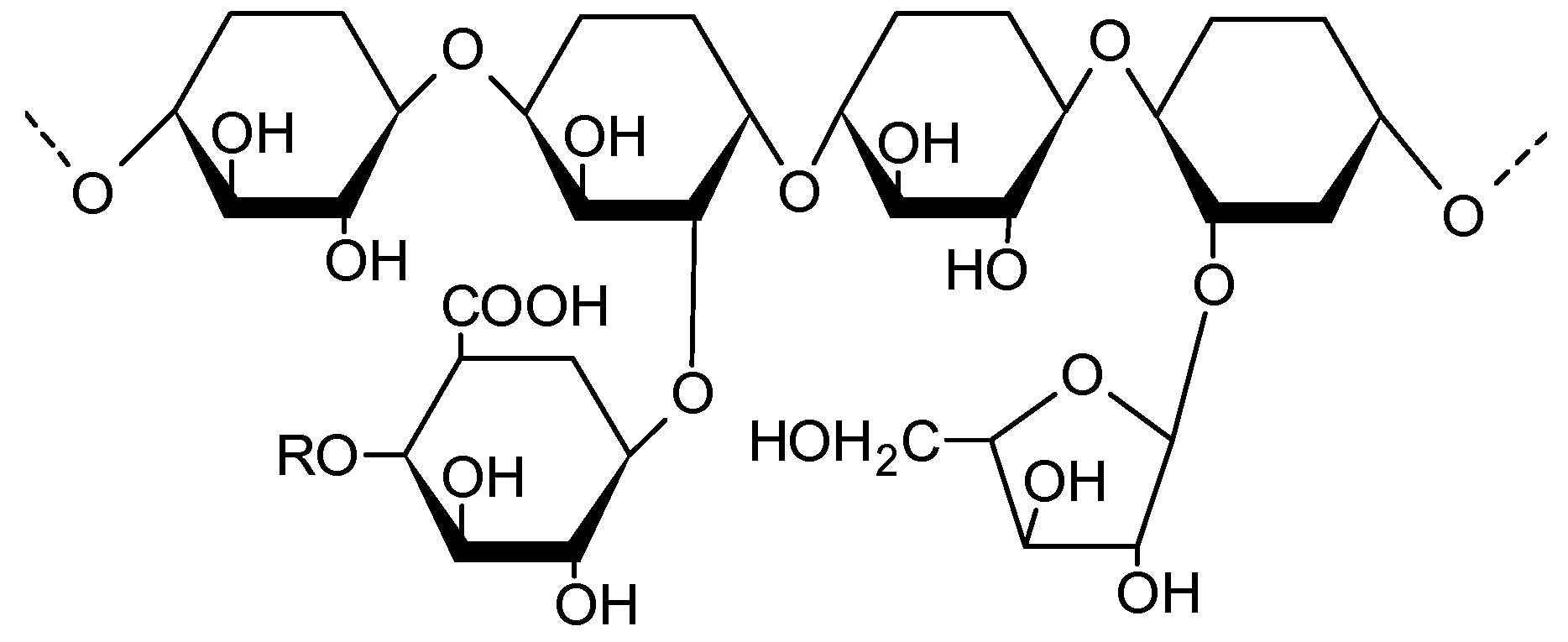
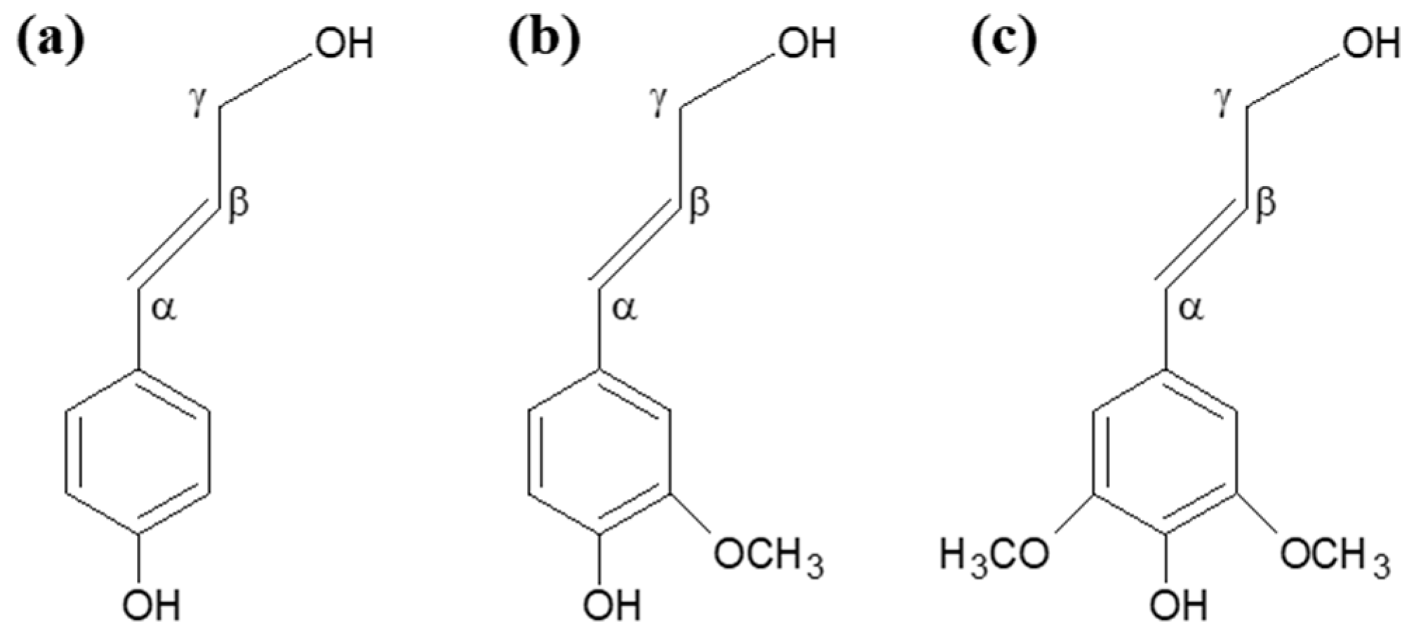
Biomass is used as a countermeasure against environmental pollution. Research has been conducted to use biomass as fuel [1], remove environmental pollution [2], or use it as an environmental improvement agent [3]. These biomass can be analysed using various methods, including elemental, proximate, and structural analyses. In the context of biomass composition, structural analysis refers to the method of analysing the contents of cellulose, hemicellulose, and lignin, which make up the biomass [4,5,6]. Cellulose is represented as [C₆H₁₀O₅]_n and consists of linear chains composed of hundreds to thousands of D-glucose units connected by beta (1→4) glycosidic bonds, as shown in Figure 1. Hemicellulose is composed of hexose sugars, such as glucose, mannose, galactose, and rhamnose, and pentose sugars, such as arabinose and xylose. They are classified based on the main sugar residues in their backbones, which can be xylan, mannan, or glucan, as shown in Figure 2. Lignin refers to hydrophobic phenolic molecules found in various components of woody plants, such as conifers and hardwoods. Precursor molecules like p-coumaryl alcohol (H), coniferyl alcohol (G), and sinapyl alcohol (S) (Figure 3) form complex three-dimensional polymer structures via β-O-4 or carbon-carbon linkages [7,8].

Previous studies have predicted calorific values of different biomass considering based on their structural characteristics. Howard [9] investigated the variation in calorific values based on different parts of pinewood and highlighted the correlation between extractives and calorific values. Tillman [10] utilised a single variable in a model to estimate the higher heating value (HHV) of wood, which was expressed as dry weight as well as on a dry ash-free basis. White [11] introduced four equations, one of which calculated the calorific value of wood-containing extractives, whereas the other three calculated the calorific values of woods without extractives. Additionally, White proposed a fifth equation inspired by Tillman’s work. Callejón-Ferre et al. [12] predicted a correlation between the structural analysis and calorific values of plant residues within greenhouses in Almería, Spain. Subsequently, predictive equations for the heating value based on structural analysis were also proposed for various biomass and thermally treated biomass.

Table 1. Models used in previous studies to predict a higher heating value (HHV) using structure analysis.

Model	Biomass	Reference
$HHV=19.307+0.118\left[E\right]$	Pine	[9]
$HHV=0.17389\left[Ho\right]+0.26629(100-\left[Ho\right])$	Extractive-free wood	[10]
$HH{V}^B=17.9017+0.0744\left[L\right]+0.0661\left[E\right]$	Unextracted wood, four softwoods and four hardwoods	[11]
$HH{V}^B=17.7481+0.0800\left[L^{\ast }\right]\left(100-\left[E\right]\right)+0.0886\left[E\right]$
$HH{V}^B=17.6132+0.0853\left[L^{\ast }\right]$	Extractive-free wood
$HH{V}^B=17.4458+0.0907\left[L^{\ast }\right]$	Extractive-free softwood
$HH{V}^B=18.0831+0.0637\left[L^{\ast }\right]$	Extractive-free hardwood
$HH{V}^B=0.0889\left[L\right]+16.8218$	Extractive-free wood and non-wood	[13]
$HH{V}^B=0.0893\left[L\right]+16.9742$	Extractive-free lignocellulosic materials
$HH{V}^B=0.0877\left[L\right]+16.4951$	Extractive-free non-wood
$HH{V}^B=0.0864\left[L\right]+16.6922$	Extractive-free sunflower shells, almond shells, hazelnut shells, wood bark, olive husks, hazelnut kernel husks, and walnut shells	[14]
$HHV=0.0979\left[L\right]+16.292$	Corn stover, corn cobs, sunflower shells, beech wood, Ailanthus wood, hazelnut shells, wood bark, olive husks, and walnut shells	[15]
$HHV=10.955+0.692\left[L\right]$	Greenhouse crops	[12]
$HHV=8.211+0.150\left[H\right]+0.767\left[L\right]$
$HHV=7.405+0.163\left[H\right]+0.065\left[C\right]+0.682\left[L\right]$
$HHV=16.1964+0.0555\left[L\right]$	Twenty biomass samples of agro-forestry wastes and industrial wastes	[16]
$HHV=17.0704-0.0202\left[H\right]+0.0449\left[L\right]$
$HHV=19.393+0.039\left[E\right]$	Tree species from Oaxaca, Mexico	[17]
$HHV=23.527-0.059\left[C\right]$
$HHV=22.582-0.051\left[C\right]+0.032\left[E\right]$
$HHV=17.893+0.068\left[L\right]$	Mixture of eight untreated and heat-treated woods	[18]

^B converted from Btu/lb; * extractive free; [C] cellulose; [H] hemicellulose; [L] lignin; [E] extractive.

summarizes some of the previous studies that predicted HHV by analysing the structure.

Equations for predicting the calorific value of heat-treated biomass have been proposed for elemental and proximate analyses [19,20]. However, few equations are available to predict the calorific value of heat-treated biomass based on structural analyses. Therefore, in this study, we aimed to present an equation for predicting the calorific value of heat-treated biomass based on structural analysis.

2. Materials and Methods

2.1. Collection of Data

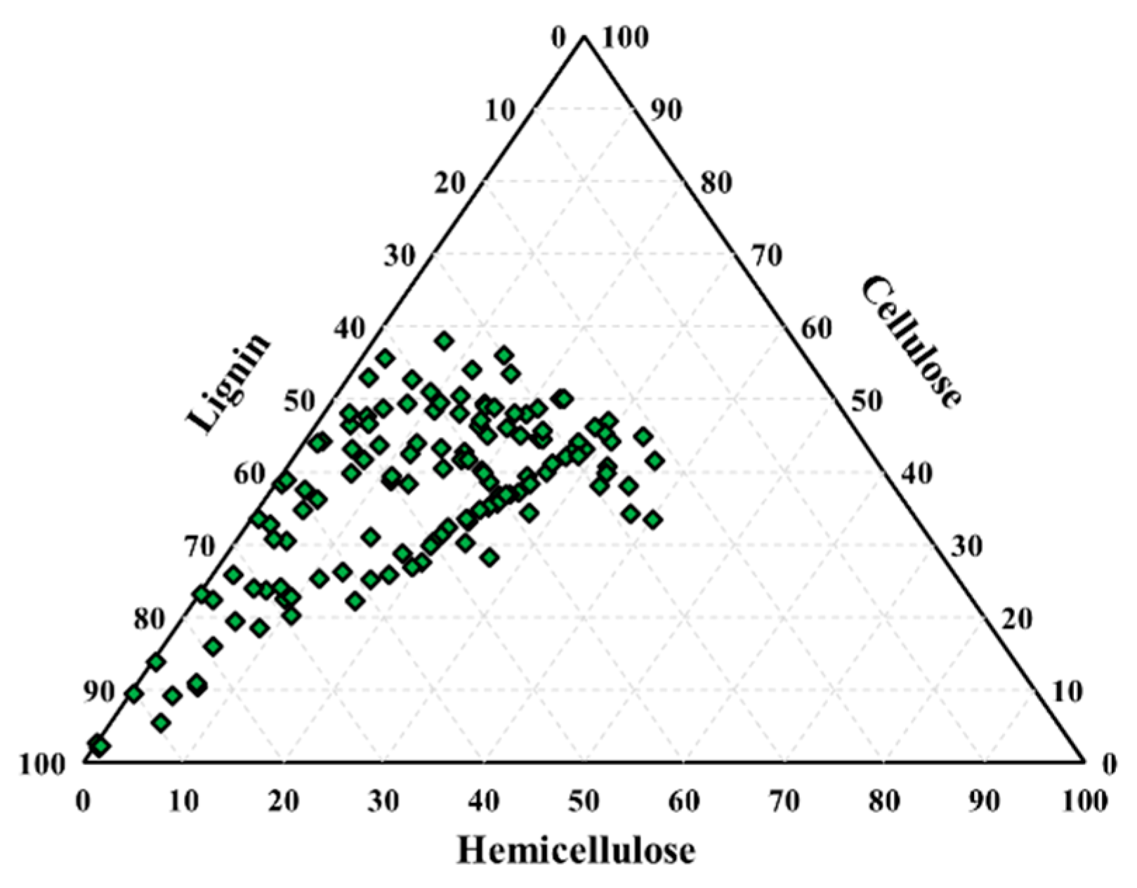
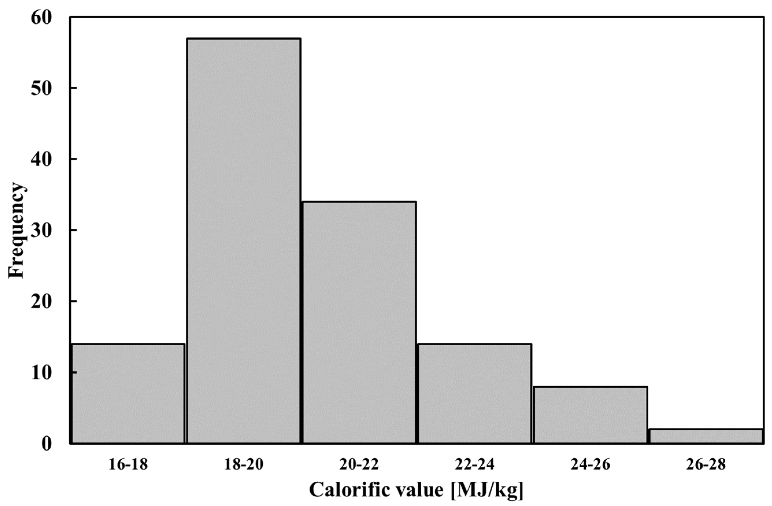
From previous studies, 111 structural analyses and calorific value data were collated for 59 woody and herbaceous biomass samples of 52 herbaceous plants [21,22,23,24,25,26,27,28,29,30,31,32,33,34,35]. All data are summarised in Table S1. The distributions of the structural composition and calorific value of the biomass are shown in Figure 4 and Figure 5.

2.2. Pearson Correlation Coefficient

The study employed the Pearson correlation coefficient (Equation (1)) to assess the relationships compositional (Cell, Hemi, and Lig) analyses and calorific value. This coefficient, as defined in Equation (1), was employed to evaluate the extent of correlation between two sets of data. It ranges from −1 to 1, where positive and negative values indicate a direct and inverse relationship, respectively. Values closer to −1 or 1 signify a stronger linear correlation, while those closer to 0 suggest a weaker correlation [36]. The analysis involved deriving correlation equations with varying goodness-of-fit values through linear and non-linear regressions applied to the final analysis data using IBM SPSS version 22.0. However, for exponential and logarithmic regression models, they were not applied due to the possibility of certain structural components becoming zero during thermal treatment. The data analysis in this study employed a combination of the “stepwise” and “enter” methods within the SPSS software. The input variables included C, H, L, squared (C², H², and L²), and squared roots (C^0.5, H^0.5, and L^0.5).

$$R=\frac{\left({\sum }_{i=1}^n\left(X_i-\overline{X}\right)\left(Y_i-\overline{Y}\right)\right)}{\sqrt{{\sum }_{i=1}^n{\left(X_i-\overline{X}\right)}^2}\sqrt{{\sum }_{i=1}^n{\left(Y_i-\overline{Y}\right)}^2}}$$

(1)

2.2.1. Linear Regression

Linear regression is a statistical approach frequently employed to ascertain the value of a dependent variable using an independent variable [37]. This method relies on a mathematical equation that yields a single value by considering a combination of input characteristics. The linear regression equation is represented as follows [38]:

$$\widehat{y}={\beta }_O+x_1{\beta }_1+x_2{\beta }_2+x_3{\beta }_3+\dots +x_n{\beta }_n$$

(2)

2.2.2. Polynomial Regression

Polynomial regression is a statistical technique in which data are approximated using a polynomial function [39]. It entails the incorporation of higher-order terms of variables to estimate the polynomial regression and construct a curved response surface [40]. As there is no universally applicable polynomial equation, the equation should be derived based on the specific problem under consideration. The general expression for a polynomial function is as follows [38]:

$$f\left(x\right)=c_o+c_{1}x+c_2{x}^2+\dots +c_n{x}^n$$

(3)

2.3. Model Evaluation

The suitability of the model was assessed using different performance metrics. Four performance metrics were used, namely the coefficient of determination (R²), mean absolute error (MAE), root-mean-squared error (RMSE), average absolute error (AAE), and average bias error (ABE). R² was employed because of its advantage in facilitating relative performance comparisons using Equation (4). This quantifies the proportion of variance in the dependent variable that is predictable from the independent variables [39]. MAE was used because it measures the absolute difference between the observed and predicted values in the same units (Equation (5)), which makes it intuitive and straightforward to interpret. RMSE has the advantage of reducing the distortion in the values resulting from squaring the errors (Equation (6)). However, its drawback is that errors < 1 become even smaller owing to squaring, whereas errors > 1 become larger. AAE and ABE represent the average errors in the correlation equation (Equations (7) and (8)). ABE is evaluated such that positive values are rated higher, indicating a better fit, whereas negative values suggest a somewhat lower fit [37,38]. These metrics provide a comprehensive evaluation of the performance of a model by considering different aspects of its accuracy and fit.

$${\mathrm{R}}^2=1-\frac{{\sum }_{\mathrm{i}=1}^{\mathrm{n}}\mathrm{V}\mathrm{a}\mathrm{l}\mathrm{u}{\mathrm{e}}_{\mathrm{M}}-\mathrm{V}\mathrm{a}\mathrm{l}\mathrm{u}{\mathrm{e}}_{\mathrm{P}}}{{\sum }_{\mathrm{i}=1}^{\mathrm{n}}\mathrm{V}\mathrm{a}\mathrm{l}\mathrm{u}{\mathrm{e}}_{\mathrm{M}}-\overline{\mathrm{V}\mathrm{a}\mathrm{l}\mathrm{u}{\mathrm{e}}_{\mathrm{P}}}},$$

(4)

$$\mathrm{M}\mathrm{A}\mathrm{E}=\frac{{\sum }_{\mathrm{i}=1}^{\mathrm{n}}\left(\mathrm{V}\mathrm{a}\mathrm{l}\mathrm{u}\mathrm{l}{\mathrm{e}}_{\mathrm{M}}-\mathrm{V}\mathrm{a}\mathrm{l}\mathrm{u}{\mathrm{e}}_{\mathrm{P}}\right)}{\mathrm{n}},$$

(5)

$$\mathrm{R}\mathrm{M}\mathrm{S}\mathrm{E}=\sqrt{\left(\frac{1}{\mathrm{n}}\right){\sum }_{\mathrm{i}=1}^{\mathrm{n}}{\left(\mathrm{V}\mathrm{a}\mathrm{l}\mathrm{u}{\mathrm{e}}_{\mathrm{M}}-\mathrm{V}\mathrm{a}\mathrm{l}\mathrm{u}{\mathrm{e}}_{\mathrm{P}}\right)}^2}$$

(6)

$$\mathrm{A}\mathrm{A}\mathrm{E}=\frac{1}{\mathrm{n}}{\sum }_{\mathrm{i}=1}^{\mathrm{n}}\left|\frac{\mathrm{V}\mathrm{a}\mathrm{l}\mathrm{u}{\mathrm{e}}_{\mathrm{P}}-\mathrm{V}\mathrm{a}\mathrm{l}\mathrm{u}{\mathrm{e}}_{\mathrm{M}}}{\mathrm{V}\mathrm{a}\mathrm{l}\mathrm{u}{\mathrm{e}}_{\mathrm{M}}}\right|,$$

(7)

$$\mathrm{A}\mathrm{B}\mathrm{E}=\frac{1}{\mathrm{n}}{\sum }_{\mathrm{i}=1}^{\mathrm{n}}\left[\frac{\mathrm{V}\mathrm{a}\mathrm{l}\mathrm{u}{\mathrm{e}}_{\mathrm{P}}-\mathrm{V}\mathrm{a}\mathrm{l}\mathrm{u}{\mathrm{e}}_{\mathrm{M}}}{\mathrm{V}\mathrm{a}\mathrm{l}\mathrm{u}{\mathrm{e}}_{\mathrm{M}}}\right],$$

(8)

Validation of the optimal conditions was conducted based on the performance metrics mentioned above, using the data listed in

Table 2. Validation data for suggested model.

Biomass	Type	Cell [%]	Hemi [%]	Lig [%]	HHV [MJ/kg]	Ref.
Mixed waste wood	Woody	38.30	25.50	22.00	17.50	[27]
Torrefied mixed waste wood (200 °C)	Woody	41.10	26.30	26.50	19.20
Torrefied mixed waste wood (250 °C)	Woody	43.70	7.70	31.40	19.90
Torrefied mixed waste wood (300 °C)	Woody	36.20	5.30	43.70	20.80
Oak waste wood	Woody	38.30	25.50	22.00	18.60
Torrefied Oak waste wood (200 °C)	Woody	41.10	26.30	26.50	19.10
Torrefied Oak waste wood (250 °C)	Woody	43.70	7.70	31.40	21.20
Torrefied Oak waste wood (300 °C)	Woody	36.20	5.30	43.70	22.50
Miscanthus	Herbaceous	41.40	19.70	22.60	16.41
Torrefied miscanthus (200 °C)	Herbaceous	41.90	21.20	23.10	19.15
Torrefied miscanthus (250 °C)	Herbaceous	44.10	8.40	41.60	21.10
Torrefied miscanthus (300 °C)	Herbaceous	35.00	3.20	52.30	21.28
Hops	Herbaceous	42.2	0	26.20	16.59
Torrefied hops (200 °C)	Herbaceous	42.9	0	26.80	18.80
Torrefied hops (250 °C)	Herbaceous	47.00	0	35.10	18.90
Torrefied hops (300 °C)	Herbaceous	39.90	0	38.70	20.70
Torrefied pine chip (225 °C)	Woody	41.23	12.87	38.42	19.48	[41]
Torrefied pine chip (250 °C)	Woody	41.90	6.93	45.70	20.08
Torrefied pine chip (275 °C)	Woody	39.54	0.99	53.30	21.82
Torrefied pine chip (300 °C)	Woody	12.84	0.56	79.99	25.38
Logging residue chip	Woody	37.49	13.26	26.15	18.79
Torrefied logging residue chip (225 °C)	Woody	41.04	14.77	33.20	19.79
Torrefied logging residue chip (250 °C)	Woody	38.57	5.87	42.49	21.21
Torrefied logging residue chip (275 °C)	Woody	34.08	5.23	52.80	22.03
Torrefied logging residue chip (300 °C)	Woody	6.10	1.04	85.06	26.41
Torrefied Cotton Balls	Herbaceous	29.44	24.22	34.20	18.73	[42]
Torrefied Sunflower	Herbaceous	31.00	29.35	24.73	19.65
Wet torrefied bamboo (180 °C 30 min 0 M HCl)	Herbaceous	42.61	25	23.18	17.79	[43]
Wet torrefied bamboo (180 °C 15 min 0.2 M HCl)	Herbaceous	34.97	0	33.94	24.19
Wet torrefied bamboo (180 °C 30 min 0.2 M HCl)	Herbaceous	13.96	0	36.98	24.86
Corn straw	Herbaceous	39.12	30.95	10.73	18.61	[44]
Torrefied corn straw (160 °C)	Herbaceous	38.03	28.86	10.12	19.17
Torrefied corn straw (180 °C)	Herbaceous	37.11	28.12	9.87	19.79
Torrefied oat hull (285 °C)	Herbaceous	33.52	0.72	45.65	22.45	[29]
Torrefied bamboo (280 °C 10 min)	Herbaceous	49.76	8.60	39.79	19.88	[45]
Torrefied bamboo (280 °C 30 min)	Herbaceous	49.40	5.56	43.12	20.11
Torrefied bamboo (280 °C 60 min)	Herbaceous	47.40	2.03	50.40	20.42
Sweet sorghum bagasse	Herbaceous	29.80	24.40	5.24	17.30	[46]
Torrefaction sweet sorghum bagasse	Herbaceous	19.90	4.80	16	23

.

To compare the optimal model selected based on the validation data with those of previous studies, we used the test dataset provided in

Table 3. Verification test dataset for comparison validation model and previous studies.

Biomass	Type	Cell [%]	Hemi [%]	Lig [%]	HHV [MJ/kg]	Ref.
Softwood	Woody	47.40	13.80	23.50	18.00	[47]
Torrefied softwood	Woody	36.60	2.65	23.20	22.30
Torrefied hardwood	Woody	46.70	1.20	15.70	22.40
Norway spruce	Woody	41.70	26.00	30.90	20.37	[46]
Torrefied Norway spruce (260 °C 8 min)	Woody	42.30	23.20	30.40	20.65
Torrefied Norway spruce (260 °C 25 min)	Woody	40.10	13.50	33.90	21.51
Corn straw	Herbaceous	39.12	30.95	10.73	18.61	[44]
Torrefied corn straw (160 °C)	Herbaceous	38.03	28.86	10.12	19.17
Torrefied miscanthus (230 °C 15 min)	Herbaceous	44.50	18.50	26.80	19.30	[48]
Torrefied miscanthus (250 °C 15 min)	Herbaceous	44.90	12.20	32.80	19.70
Torrefied miscanthus (250 °C 30 min)	Herbaceous	43.30	9.90	36.20	19.90
Torrefied willow (230 °C 15 min)	Woody	39.70	18.10	28.70	19.60
Torrefied willow (250 °C 15 min)	Woody	40.50	15.30	30.30	19.90
Torrefied willow (270 °C 15 min)	Woody	41.10	12.90	33.40	20.20
Torrefied willow (230 °C 30 min)	Woody	39.30	16.80	29.60	19.60
Torrefied willow (250 °C 30 min)	Woody	40.30	14.70	31.40	19.80
Torrefied willow (270 °C 30 min)	Woody	41.60	14.20	32.90	20.50
Bamboo	Herbaceous	48.03	24.13	27.83	19.00	[49]
Wet torrefied bamboo (200 °C)	Herbaceous	50.22	22.68	27.10	19.40
Wet torrefied bamboo (220 °C)	Herbaceous	49.88	25.09	25.03	19.60
Dry torrefied bamboo (180 °C)	Herbaceous	43.13	25.04	31.84	19.10
Dry torrefied bamboo (200 °C)	Herbaceous	36.78	27.96	35.25	19.40

for verification.

3. Results and Discussion

3.1. Result of Pearson Correlation Coefficient

The results of the Pearson’s correlation coefficient are summarized in Figure 6. In the case of cellulose, a positive correlation was observed with hemicellulose, while a negative correlation was found with calorific value. The reason for the positive correlation between hemicellulose and cellulose is likely because they share precursor structures composed of pentose or hexose sugar monomers. For hemicellulose, there was a negative correlation with calorific value and lignin. Particularly, the strong negative correlation of −0.7668 with lignin suggests that in heat-treated samples, the presence of hemicellulose decreases while the lignin content increases due to the decomposition of hemicellulose. In the case of cellulose, it decomposes at high temperatures and decreases like hemicellulose, which is inversely proportional to the increase in HHV. However, due to lower decomposition rate compared with hemicellulose, it has a negative correlation, but it appears to be a weaker correlation than the correlation between hemicellulose and HHV. Lignin, on the other hand, exhibited a strong positive correlation of 0.6518 with the calorific value. This can be attributed to the fact that lignin is a polymer with a high carbon content, and in heat-treated samples, the lignin content tends to be higher, leading to an increase in calorific value.

3.2. Prediction Model Using Total Biomass

The equations for predicting the calorific value of the overall biomass are summarised in

Table 4. Calorific value prediction model using overall lignocellulosic biomass.

No.	Equation	R2P [-] 1	RMSEP [-] 2	MAEP [%] 3	AAEP [%] 4	ABEP [%] 5
T1	$HHV=22.011-0.649H^{0.5}+0.0000424L^2$	0.5423	1.3858	1.1006	5.3455	0.4302
T2	$\begin{array}{ll}HHV=-4.205-& 0.003C^2+0.576C-1.931C^{0.5}\\ & +0.003H^2-0.589H+7.491H^{0.5}\\ & +0.007L^2-1.337L+10.134L^{0.5}\\ & +0.013CH-1.313C{H}^{0.5}\end{array}$	0.5719	1.5215	1.1764	5. 7280	2.1895
T3	$\begin{array}{ll}HHV=-2.918+& 0.228C-0.269H+5.553H^{0.5}\\ & -1.115L+0.006L^2+8.469L^{0.5}\\ & +0.01CH-1.138C{H}^{0.5}\end{array}$	0.5814	1.5455	1.1924	5.8641	2.9964

¹ coefficient of determination, ² root mean square error, ³ mean absolute error, ⁴ average absolute error, ⁵ average bias error.

. Given the diverse characteristics of the various biomass samples, they exhibited substantial variations, which likely contributed to the lower R² values. Various input variables were applied, and the highest R²_P value of 0.5814 was obtained for T3.

T1 and T2 had an R²_P value of 0.5423 and 0.5719, respectively. T3 had the highest value of RMSE_P at 1.5455, whereas T1 had the lowest RMSE_P of 1.3858. AAE_P for T1 was calculated as 5.3455%. However, T2 and T3 exhibited an error rate of 5.7280% and 5.8641%, respectively. Furthermore, among the prediction models that used the overall biomass, the predicted values were higher, resulting in positive ABE_P values. T1 exhibited the lowest ABE_P of 0.4302%. Hence, T2 predicted more accurately than the ABE_P of T2 and T3, which were 2.1895% and 2.9964%, respectively. Given that the performance metrics did not meet the desired level of accuracy, a decision was made to enhance the model’s performance by separating the predictions for woody and herbaceous biomass. This separation was undertaken as the simultaneous prediction of both hardwoods and softwoods may have contributed to the reduced accuracy observed in the model.

3.3. Prediction Model Using Woody Biomass

Three prediction models for woody biomass are presented in

Table 5. Calorific value prediction model using woody biomass.

No.	Equation	R2P [-]	RMSEP [-]	MAEP [%]	AAEP [%]	ABEP [%]
W1	$\begin{array}{ll}HHV=31.257-& 0.039C+0.001C^2-0.88C^{0.5}\\ & +0.074H-0.001H^2-1.738H^{0.5}\\ & -0.001L^2+0.463L^{0.5}\end{array}$	0.7811	1.2810	1.0860	5.3534	2.8879
W2	$\begin{array}{ll}HHV=31.027+& 0.000316C^2-1.118C^{0.5}-1.398H^{0.5}\\ & -0.001L^2+0.462L^{0.5}\end{array}$	0.8222	1.1888	0.8724	4.0008	−1.7930
W3	$HHV=27.567-0.28C^{0.5}-1.333H^{0.5}$	0.8392	0.9626	0.7238	3.5106	0.2286

. When compared to the previous prediction models for lignocellulosic biomass, the R²_P values for woody biomass were notably higher, ranging from 0.82 to 0.83. Similarly, the RMSE_P values for these models fell within the range of 0.96 to 1.18.

Interestingly, in most cases, an increase in the number of input variables tended to result in higher R²_P values, which could indicate a risk of overfitting. However, it is worth noting that for the prediction models of woody biomass, the model with the highest number of input variables, W1, exhibited the lowest R²_P value and the highest RMSE_P. On the contrary, the model with the fewest input variables, W3, demonstrated reasonable performance, boasting an R²_P of 0.8392 and an RMSE_P of 0.9626.

3.4. Prediction Model for Herbaceous Biomass

The prediction models for herbaceous biomass are outlined in

Table 6. Calorific value prediction model using herbaceous biomass.

No.	Equation	R2P [-]	RMSEP [-]	MAEP [%]	AAEP [%]	ABEP [%]
H1	$\begin{array}{ll}HHV=24.918+& 0.002H{o}^2-1.36H{o}^{0.5}+2.813H^{0.5}\\ & -0.003L^2+0.165L-0.67C{H}^{0.5}\end{array}$	0.8256	1.2958	1.1723	5.9563	−5.8252
H2	$\begin{array}{ll}HHV=15.513+& 0.002C^2-1.283C^{0.5}-0.297H\\ & +0.007H^2+2.688H^{0.5}-0.388L\\ & +4.23L^{0.5}+0.003CH-0.504C{H}^{0.5}\end{array}$	0.8561	0.6294	0.5243	2.7030	1.8674
H3	$\begin{array}{ll}HHV=14.738+& 0.002C^2-1.246C^{0.5}+0.007H^2\\ & -0.31H+2.8H^{0.5}-0.429L\\ & +4.524L^{0.5}+0.003CH-0.521C{H}^{0.5}\end{array}$	0.8739	0.4836	0.3698	1.8929	−0.2333

. The R²_P values for these models varied in the range of 0.82 to 0.87. Interestingly, the model with the fewest input variables, H1, had the lowest R²_P, whereas the model with the most input variables, H3, had the highest R²_P. However, when considering the RMSE_P, H1 had the highest value at 1.2958. In terms of ABE_P, only H2 had a positive value, while H1 and H3 had negative values, indicating an underestimation in the latter cases. The reason for the low accuracy of herbaceous biomass was due to be extractive and non-uniformity compared with woody biomass. In general, it is known that the extractive and ash content of herbaceous biomass is higher than that of woody biomass [50,51]. Because this was not considered in this study, it was determined to be low.

3.5. Validation of Calorific Value Prediction Models

A validation process was carried out to determine the most suitable model among the presented models.

Table 7. Validation of the results obtained from the model using overall lignocellulosic biomass.

	R2CV [-]	RMSECV [-]	MAECV [%]	AAECV [%]	ABECV [%]
T1	0.4920	1.9178	1.3871	6.6409	0.3278
T2	0.7870	1.1258	0.9180	4.3728	0.3878
T3	0.4902	1.9198	1.4490	7.0107	1.2695

displays the validation outcomes for overall lignocellulosic biomass. The validation results reveal that T2 achieved the highest R²_CV, standing at 0.7870. However, it also displayed the lowest RMSE_CV, which was 1.1258. Both T1 and T3 demonstrated R²_CV values of approximately 0.4920. Comparing MAE_CV and AAE_CV, T2 demonstrated satisfactory performances. In conclusion, based on the validation results, T2 emerged as the optimal model.

Regarding woody biomass (

Table 8. Validation of the results obtained from the model using woody biomass.

	R2CV [-]	RMSECV [-]	MAECV [%]	AAECV [%]	ABECV [%]
W1	0.6217	2.0387	1.8632	9.1077	7.6093
W2	0.6933	1.4568	1.2382	5.9518	3.7659
W3	0.8108	1.4423	1.2070	5.9422	5.2810

), most models displayed R²_CV values within the range of 0.60 to 0.69. However, W3 stood out with the highest R²_CV value of 0.8108. The RMSE_CV values generally fell between 1.44 and 1.45 for most models, although W1 had a slightly higher RMSE_CV at 2.0387. When considering ABE_CV, W3 had the highest value, reaching 5.2810, compared to W1 and W2 with values of 3.7659. Despite its higher ABE_CV, W3 was deemed the optimal choice due to its combination of a high R²_CV, low RMSE_CV, and a reduced number of input variables.

In the case of herbaceous biomass (

Table 9. Validation of the results obtained from the model using woody biomass.

	R2CV [-]	RMSECV [-]	MAECV [%]	AAECV [%]	ABECV [%]
H1	0.8959	2.1312	1.9740	9.4032	−9.3217
H2	0.8528	1.3266	1.0707	5.0002	−3.5535
H3	0.8672	1.5457	1.3415	6.2997	−5.3494

), the R²_CV values were notably higher, increasing within the range of 0.528 to 0.8959. Additionally, their RMSE_CV values ranged from 1.3266 to 2.1312, respectively. The R²_cv of H1 was the highest at 0.8959, but RMSE_CV was 2.1312, higher than H2’s 1.3266. H2 and H3 showed better performance in RMSE_CV, MAE_CV, AAE_CV, and ABE_CV. Despite a lower R²_cv, H2 was determined to be optimal.

3.6. Comparison of the Model with Previous Models

Using a verification dataset, we conducted a comparison between the calorific value prediction model developed in our study and models from previous research. For this study, we chose the model by Demirbaş [13], which was based on non-wood biomass, and the model by Domingos et al. [18], which utilized equations formulated using heat-treated biomass.

The biomass test results are outlined in

Table 10. Validation of the results obtained from the model using overall biomass.

	Equation	R2	RMSE	MAE	AAE	ABE
T2	$\begin{array}{ll}HHV=-4.205-& 0.003C^2+0.576C-1.931C^{0.5}\\ & +0.003H^2-0.589H+7.491H^{0.5}\\ & +0.007L^2-1.337L+10.134L^{0.5}\\ & +0.013CH-1.313C{H}^{0.5}\end{array}$	0.5171	0.7702	0.5768	2.9346	−0.2742
Demirbaş [13]	$HH{V}^B=0.0877\left[L\right]+16.4951$	0.0058	1.3534	0.8719	4.2037	−3.1029
Domingos et al. [18]	$HHV=17.893+0.068\left[L\right]$	0.0058	1.1299	0.7384	3.5927	−0.4441

. The RMSE values for T2, Demirbaş [13], and Domingos et al. [18] were recorded as 0.7702, 1.3534, and 1.1298, respectively. The T2 model proposed in our study exhibited the lowest RMSE. In the case of torrefied biomass, Domingos et al. [18] displayed a lower RMSE compared to Demirbaş [13]. The R² values were relatively low due to the variations in biomass properties, with a notably low R² value of 0.0059 observed in previous studies. Since both previous studies predicted only lignin as a variable, R² was observed to have the same value. In the case of previous studies, it was predicted based on lignin alone, but other studies indicate that there are other properties that have significant weight in changes in HHV in addition to lignin [50,52]. Through actual analysis, it was confirmed that cellulose and hemicellulose affected HHV. In all model, a negative ABE was noted, indicating an underestimation, as depicted in Figure 7a.

In the case of woody biomass (

Table 11. Comparison of the model with those defined in previous studies by using woody biomass test dataset.

	Equation	R2	RMSE	MAE	AAE	ABE
W3	$HHV=27.567-0.28C^{0.5}-1.333H^{0.5}$	0.4152	1.2668	1.0902	5.3992	2.7024
Demirbaş [13]	$HH{V}^B=0.0877\left[L\right]+16.4951$	0.0894	1.7427	1.2145	5.7017	−4.8843
Domingos et al. [18]	$HHV=17.893+0.068\left[L\right]$	0.0894	1.4359	0.9479	4.4850	−2.3996

), the W3 model proposed in our study displayed the lowest RMSE. Conversely, the Demirbaş equation had a higher RMSE of 1.7427 compared to the other two equations. Also, the R² value was higher for W3, measuring 0.4152. When considering ABE, W3 was the only equation with a positive value, while that of Demirbaş exhibited a significantly negative value of −4.8843%, indicating an underestimation. Consequently, as depicted in Figure 7b, W3 is represented by a positive trendline, whereas the two equations from previous studies exhibit negative trends.

For herbaceous biomass (

Table 12. Comparison of the model with those defined in previous studies by using herbaceous biomass test dataset.

	Equation	R2	RMSE	MAE	AAE	ABE
H1	$\begin{array}{ll}HHV=15.513+& 0.002C^2-1.283C^{0.5}-0.297H\\ & +0.007H^2+2.688H^{0.5}\\ & -0.388L+4.23L^{0.5}+0.003CH\\ & -0.504C{H}^{0.5}\end{array}$	0.0830	0.5176	0.4677	2.4114	−0.8891
Demirbaş [13]	$HH{V}^B=0.0877\left[L\right]+16.4951$	0.4382	0.6208	0.4608	2.4060	−0.9652
Domingos et al. [18]	$HHV=17.893+0.068\left[L\right]$	0.4382	0.5784	0.4869	2.5220	1.9026

), H1 showed an RMSE of 0.5176, whereas Domingos et al. [18] reported an RMSE of 0.5784. The Demirbaş equation exhibited the highest RMSE among the three at 0.6208. However, the R² value for the Demirbaş and Domingos et al. equation was the highest. Regarding the ABE, only the H1 and Demirbaş equation showed negative values, whereas the Domingos et al. equation had positive values. This is illustrated in Figure 7c. The trend line of Domingos et al. exhibited an upward positive trend, suggesting that predictions from the equations tended to overestimate the values. In contrast, the Demirbaş equation and H1 resulted in an underestimation.

4. Conclusions

In this study, the calorific value of lignocellulose using structural analyses was predicted. Building on previous research, we predicted the calorific value by classifying biomass as overall lignocellulose biomass, woody biomass, and herbaceous biomass. When using the overall biomass dataset, the presented models yielded relatively low R²_P values, ranging from 0.5423 to 0.5814. However, when analysing the models separately for woody and herbaceous biomass, R² values of woody biomass ranged from 0.7811 to 0.8392, and those of herbaceous biomass ranged from 0.8256 to 0.8739.

The optimal model was identified after validation. Equations (9)–(11) were identified as the optimal model equations.

$$\begin{array}{ll}HHV=-4.205-& 0.003C^2+0.576C-1.931C^{0.5}+0.003H^2-0.589H\\ & +7.491H^{0.5}+0.007L^2-1.337L+10.134L^{0.5}+0.013CH\\ & -1.313C{H}^{0.5}\end{array}$$

(9)

$$HHV=27.567-0.28C^{0.5}-1.333H^{0.5}$$

(10)

$$\begin{array}{ll}HHV=24.918+& 0.002H{o}^2-1.36H{o}^{0.5}+2.813H^{0.5}-0.003L^2+0.165L\\ & -0.67C{H}^{0.5}\end{array}$$

(11)

Furthermore, the chosen equations were assessed using a test dataset, revealing that T1 and W3 exhibited improved performance compared to previous studies, while H1 showed lower performance compared to prior research. Although the R² of H1 was low, the RMSE was low compared to previous studies, so it is seemed to be sufficiently usable. In the case of other studies, they were conducted in an extractive-free biomass, but it is important to note that this study presented a calorific value prediction model that did not consider extractive-free biomass. Also, the accuracy of the model using cellulose, hemicellulose, and lignin was confirmed to be higher than that of the conventional lignin-based calorific value prediction model.

This study aimed to encompass various biomass types but was based on a dataset of 111 biomass samples for model construction. However, the prediction rates for calorific values were relatively low for herbaceous and lignocellulosic biomass datasets. Future research should prioritize the development of models capable of predicting cellulose, hemicellulose, lignin, and calorific values across various biomass types and a wide range of heat treatment conditions.

References

1. Park, S.; Kim, S.J.; Oh, K.C.; Jeon, Y.K.; Kim, Y.; Cho, A.Y.; Lee, D.; Jang, C.S.; Kim, D.H. Biochar from Agro-Byproducts for Use as a Soil Amendment and Solid Biofuel. J. Biosyst. Eng. 2023, 48, 93–103. [Google Scholar] [CrossRef]
2. Jia, L.; Cheng, P.; Yu, Y.; Chen, S.-H.; Wang, C.-X.; He, L.; Nie, H.-T.; Wang, J.-C.; Zhang, J.-C.; Fan, B.-G.; et al. Regeneration Mechanism of a Novel High-Performance Biochar Mercury Adsorbent Directionally Modified by Multimetal Multilayer Loading. J. Environ. Manag. 2023, 326, 116790. [Google Scholar] [CrossRef]
3. Park, S.; Kim, S.J.; Cho, A.Y.; Kim, Y.; Lee, D.H.; Oh, K.C.; Jang, C.S.; Kim, D.H. Effect of Agro-byproduct Biochar Fertilization on Cherry Tomato Growth and Carbon Sequestration. J. Agric. Life Environ. Sci. 2022, 34, 229–237. [Google Scholar] [CrossRef]
4. Motta, I.L.; Miranda, N.T.; Maciel Filho, R.; Wolf Maciel, M.R. Biomass Gasification in Fluidized Beds: A Review of Biomass Moisture Content and Operating Pressure Effects. Renew. Sustain. Energy Rev. 2018, 94, 998–1023. [Google Scholar] [CrossRef]
5. Gardner, K.H.; Blackwell, J. The Structure of Native Cellulose. Biopolymers 1974, 13, 1975–2001. [Google Scholar] [CrossRef]
6. Yeo, J.Y.; Chin, B.L.F.; Tan, J.K.; Loh, Y.S. Comparative Studies on the Pyrolysis of Cellulose, Hemicellulose, and Lignin Based on Combined Kinetics. J. Energy Inst. 2019, 92, 27–37. [Google Scholar] [CrossRef]
7. Ralph, J.; Lapierre, C.; Boerjan, W. Lignin Engineering-Special Issue for Lignin Structure and Its Engineering. Curr. Opin. Biotechnol. 2019, 56, 240–249. [Google Scholar] [CrossRef]
8. Vanholme, R.; Morreel, K.; Ralph, J.; Boerjan, W. Lignin Engineering. Curr. Opin. Plant Biol. 2008, 11, 278–285. [Google Scholar] [CrossRef]
9. Howard, E.T. Heat of Combustion of Various Southern Pine Materials. Wood Sci. 1973, 5, 194–197. [Google Scholar]
10. Tillman, D.A. Wood as an Energy Resource; Academic Press: New York, NY, USA, 1978. [Google Scholar]
11. White, R.H. Effect of lignin content and extractives on the higher heating value of wood. Wood Fiber. Sci. 1987, 19, 446–452. [Google Scholar]
12. Callejón-Ferre, A.J.; Carreño-Sánchez, J.; Suárez-Medina, F.J.; Pérez-Alonso, J.; Velázquez-Martí, B. Prediction Models for Higher Heating Value Based on the Structural Analysis of the Biomass of Plant Remains from the Greenhouses of Almería (Spain). Fuel 2014, 116, 377–387. [Google Scholar] [CrossRef]
13. Demirbas, A. Relationships between Lignin Contents and Heating Values of Biomass. Energy Convers. Manag. 2001, 42, 183–188. [Google Scholar] [CrossRef]
14. Demirbaş, A. Biodiesel Fuels from Vegetable Oils via Catalytic and Non-Catalytic Supercritical Alcohol Transesterifications and Other Methods: A Survey. Energy Convers. Manag. 2003, 44, 2093–2109. [Google Scholar] [CrossRef]
15. Acar, S.; Ayanoglu, A. Determination of Higher Heating Values (HHVs) of Biomass Fuels. Energy Educ. Sci. Technol. Part A Energy Sci. Res. 2012, 28, 749–758. [Google Scholar]
16. Álvarez, A.; Pizarro, C.; García, R.; Bueno, J.L. Spanish Biofuels Heating Value Estimation Based on Structural Analysis. Ind. Crops Prod. 2015, 77, 983–991. [Google Scholar] [CrossRef]
17. Ruiz-Aquino, F.; Ruiz-Ángel, S.; Feria-Reyes, R.; Santiago-García, W.; Suárez-Mota, M.E.; Rutiaga-Quiñones, J.G. Wood Chemical Composition of Five Tree Species from Oaxaca, Mexico. Bioresources 2019, 14, 9826–9839. [Google Scholar] [CrossRef]
18. Domingos, I.; Ayata, U.; Ferreira, J.; Cruz-Lopes, L.; Sen, A.; Sahin, S.; Esteves, B. Calorific Power Improvement of Wood by Heat Treatment and Its Relation to Chemical Composition. Energies 2020, 13, 5322. [Google Scholar] [CrossRef]
19. Qian, C.; Li, Q.; Zhang, Z.; Wang, X.; Hu, J.; Cao, W. Prediction of Higher Heating Values of Biochar from Proximate and Ultimate Analysis. Fuel 2020, 265, 116925. [Google Scholar] [CrossRef]
20. Oh, K.C.; Kim, J.; Park, S.Y.; Kim, S.J.; Cho, L.H.; Lee, C.G.; Roh, J.; Kim, D.H. Development and Validation of Torrefaction Optimization Model Applied Element Content Prediction of Biomass. Energy 2021, 214, 119027. [Google Scholar] [CrossRef]
21. Ben, H.; Ragauskas, A.J. Torrefaction of Loblolly Pine. Green Chem. 2012, 14, 72–76. [Google Scholar] [CrossRef]
22. Cahyanti, M.N.; Doddapaneni, T.R.K.C.; Madissoo, M.; Pärn, L.; Virro, I.; Kikas, T. Torrefaction of Agricultural and Wood Waste: Comparative Analysis of Selected Fuel Characteristics. Energies 2021, 14, 2774. [Google Scholar] [CrossRef]
23. Lin, Y.Y.; Chen, W.H.; Colin, B.; Pétrissans, A.; Lopes Quirino, R.; Pétrissans, M. Thermodegradation Characterization of Hardwoods and Softwoods in Torrefaction and Transition Zone between Torrefaction and Pyrolysis. Fuel 2022, 310, 122281. [Google Scholar] [CrossRef]
24. Reza, M.T.; Uddin, M.H.; Lynam, J.G.; Coronella, C.J. Engineered Pellets from Dry Torrefied and HTC Biochar Blends. Biomass Bioenergy 2014, 63, 229–238. [Google Scholar] [CrossRef]
25. Arous, S.; Koubaa, A.; Bouafif, H.; Bouslimi, B.; Braghiroli, F.L.; Bradai, C. Effect of Pyrolysis Temperature and Wood Species on the Properties of Biochar Pellets. Energies 2021, 14, 6529. [Google Scholar] [CrossRef]
26. Chin, K.L.; H’ng, P.S.; Go, W.Z.; Wong, W.Z.; Lim, T.W.; Maminski, M.; Paridah, M.T.; Luqman, A.C. Optimization of Torrefaction Conditions for High Energy Density Solid Biofuel from Oil Palm Biomass and Fast Growing Species Available in Malaysia. Ind. Crops Prod. 2013, 49, 768–774. [Google Scholar] [CrossRef]
27. Ivanovski, M.; Goricanec, D.; Krope, J.; Urbancl, D. Torrefaction Pretreatment of Lignocellulosic Biomass for Sustainable Solid Biofuel Production. Energy 2022, 240, 122483. [Google Scholar] [CrossRef]
28. Chen, W.H.; Hsu, H.C.; Lu, K.M.; Lee, W.J.; Lin, T.C. Thermal Pretreatment of Wood (Lauan) Block by Torrefaction and Its Influence on the Properties of the Biomass. Energy 2011, 36, 3012–3021. [Google Scholar] [CrossRef]
29. Valdez, E.; Tabil, L.G.; Mupondwa, E.; Cree, D.; Moazed, H. Microwave Torrefaction of Oat Hull: Effect of Temperature and Residence Time. Energies 2021, 14, 4298. [Google Scholar] [CrossRef]
30. Granados, D.A.; Ruiz, R.A.; Vega, L.Y.; Chejne, F. Study of Reactivity Reduction in Sugarcane Bagasse as Consequence of a Torrefaction Process. Energy 2017, 139, 818–827. [Google Scholar] [CrossRef]
31. Ma, Z.; Zhang, Y.; Shen, Y.; Wang, J.; Yang, Y.; Zhang, W.; Wang, S. Oxygen Migration Characteristics during Bamboo Torrefaction Process Based on the Properties of Torrefied Solid, Gaseous, and Liquid Products. Biomass Bioenergy 2019, 128, 105300. [Google Scholar] [CrossRef]
32. Kanwal, S.; Chaudhry, N.; Munir, S.; Sana, H. Effect of Torrefaction Conditions on the Physicochemical Characterization of Agricultural Waste (Sugarcane Bagasse). Waste Manag. 2019, 88, 280–290. [Google Scholar] [CrossRef]
33. Xu, F.; Linnebur, K.; Wang, D. Torrefaction of Conservation Reserve Program Biomass: A Techno-Economic Evaluation. Ind. Crops Prod. 2014, 61, 382–387. [Google Scholar] [CrossRef]
34. Joshi, Y.; Di Marcello, M.; De Jong, W. Torrefaction: Mechanistic Study of Constituent Transformations in Herbaceous Biomass. J. Anal. Appl. Pyrolysis 2015, 115, 353–361. [Google Scholar] [CrossRef]
35. Chen, C.; Qu, B.; Wang, W.; Wang, W.; Ji, G.; Li, A. Rice Husk and Rice Straw Torrefaction: Properties and Pyrolysis Kinetics of Raw and Torrefied Biomass. Environ. Technol. Innov. 2021, 24, 101872. [Google Scholar] [CrossRef]
36. Chicco, D.; Warrens, M.J.; Jurman, G. The Coefficient of Determination R-Squared Is More Informative than SMAPE, MAE, MAPE, MSE and RMSE in Regression Analysis Evaluation. PeerJ Comput. Sci. 2021, 7, e623. [Google Scholar] [CrossRef]
37. Majumder, A.K.; Jain, R.; Banerjee, P.; Barnwal, J.P. Development of a New Proximate Analysis Based Correlation to Predict Calorific Value of Coal. Fuel 2008, 87, 3077–3081. [Google Scholar] [CrossRef]
38. Elmaz, F.; Yücel, Ö.; Mutlu, A.Y. Makine Öğrenmesi Ile Kısa ve Elemental Analiz Kullanarak Katı Yakıtların Üst Isı Değerinin Tahmin Edilmesi. Int. J. Adv. Eng. Pure Sci. 2020, 32, 145–151. [Google Scholar] [CrossRef]
39. Zhang, T.; Zhang, Q.; Wang, Q. Model Detection for Functional Polynomial Regression. Comput. Stat. Data Anal. 2014, 70, 183–197. [Google Scholar] [CrossRef]
40. Gendy, T.S.; El-Shiekh, T.M.; Zakhary, A.S. A Polynomial Regression Model for Stabilized Turbulent Confined Jet Diffusion Flames Using Bluff Body Burners. Egypt. J. Pet. 2015, 24, 445–453. [Google Scholar] [CrossRef]
41. Phanphanich, M.; Mani, S. Impact of Torrefaction on the Grindability and Fuel Characteristics of Forest Biomass. Bioresour. Technol. 2011, 102, 1246–1253. [Google Scholar] [CrossRef]
42. Akhtar, J.; Imran, M.; Ali, A.M.; Nawaz, Z.; Muhammad, A.; Butt, R.K.; Jillani, M.S.; Naeem, H.A. Torrefaction and Thermochemical Properties of Agriculture Residues. Energies 2021, 14, 4218. [Google Scholar] [CrossRef]
43. Li, M.F.; Shen, Y.; Sun, J.K.; Bian, J.; Chen, C.Z.; Sun, R.C. Wet Torrefaction of Bamboo in Hydrochloric Acid Solution by Microwave Heating. ACS Sustain. Chem. Eng. 2015, 3, 2022–2029. [Google Scholar] [CrossRef]
44. Li, Y.; Fan, X.; Zhang, H.; Ai, F.; Jiao, Y.; Zhang, Q.; Zhang, Z. Pretreatment of Corn Stover by Torrefaction for Improving Reducing Sugar and Biohydrogen Production. Bioresour. Technol. 2022, 351, 126905. [Google Scholar] [CrossRef] [PubMed]
45. Li, M.F.; Chen, C.Z.; Li, X.; Shen, Y.; Bian, J.; Sun, R.C. Torrefaction of Bamboo under Nitrogen Atmosphere: Influence of Temperature and Time on the Structure and Properties of the Solid Product. Fuel 2015, 161, 193–196. [Google Scholar] [CrossRef]
46. Strandberg, M.; Olofsson, I.; Pommer, L.; Wiklund-Lindström, S.; Åberg, K.; Nordin, A. Effects of Temperature and Residence Time on Continuous Torrefaction of Spruce Wood. Fuel Process. Technol. 2015, 134, 387–398. [Google Scholar] [CrossRef]
47. Mafu, L.D.; Neomagus, H.W.J.P.; Everson, R.C.; Carrier, M.; Strydom, C.A.; Bunt, J.R. Structural and Chemical Modifications of Typical South African Biomasses during Torrefaction. Bioresour. Technol. 2016, 202, 192–197. [Google Scholar] [CrossRef] [PubMed]
48. Grams, J.; Kwapińska, M.; Jędrzejczyk, M.; Rzeźnicka, I.; Leahy, J.J.; Ruppert, A.M. Surface Characterization of Miscanthus × Giganteus and Willow Subjected to Torrefaction. J. Anal. Appl. Pyrolysis 2019, 138, 231–241. [Google Scholar] [CrossRef]
49. Yang, W.; Wu, S.; Wang, H.; Ma, P.; Shimanouchi, T.; Kimura, Y.; Zhou, J. Effect of Wet and Dry Torrefaction Process on Fuel Properties of Solid Fuels Derived from Bamboo and Japanese Cedar. Bioresources 2017, 12, 8629–8640. [Google Scholar] [CrossRef]
50. Smit, A.; Huijgen, W. Effective Fractionation of Lignocellulose in Herbaceous Biomass and Hardwood Using a Mild Acetone Organosolv Process. Green Chem. 2017, 19, 5505–5514. [Google Scholar] [CrossRef]
51. Thammasouk, K.; Tandjo, D.; Penner, M.H. Influence of Extractives on the Analysis of Herbaceous Biomass†. J. Agric. Food Chem. 1997, 45, 437–443. [Google Scholar] [CrossRef]
52. Enes, T.; Aranha, J.; Fonseca, T.; Lopes, D.; Alves, A.; Lousada, J. Thermal Properties of Residual Agroforestry Biomass of Northern Portugal. Energies 2019, 12, 1418. [Google Scholar] [CrossRef]
Figure 1. Structure of cellulose.
Energies 16 07896 g001
Figure 2. Structure of hemicellulose (arabinoglucuronoxylans).
Energies 16 07896 g002
Figure 3. Structure of (a) p-coumaryl alcohol; (b) coniferyl alcohol; and (c) sinapyl alcohol.
Energies 16 07896 g003
Figure 4. Scatter plot of structural composition of biomass.
Energies 16 07896 g004
Figure 5. Histogram of calorific value.
Energies 16 07896 g005
Figure 6. Result of Pearson correlation coefficient.
Energies 16 07896 g006
Figure 7. Scatter plot for predicted and observed calorific values when different biomass types were used: (a) overall lignocellulosic biomass, (b) woody biomass, (c) herbaceous biomass [13,18].
Energies 16 07896 g007