Article

Experimental and Numerical Evaluation of Solar Receiver Heat Losses of a Commercial 9 MWe Linear Fresnel Power Plant

1
Processes, Materials and Solar Energy Laboratory, PROMES-CNRS, 7 Rue du Four Solaire, 66120 Font Romeu, France
2
eLLO Solar Power Plant, Port de Llo, 66800 Llo, France
*
Author to whom correspondence should be addressed.
Energies 2023, 16(23), 7912; https://doi.org/10.3390/en16237912
Submission received: 10 October 2023 / Revised: 10 November 2023 / Accepted: 27 November 2023 / Published: 4 December 2023
(This article belongs to the Special Issue Advanced Solar Thermal Technology)

Abstract

:
Evaluating the heat losses of linear Fresnel concentrator (LFC) receivers is crucial for determining plant efficiency and managing the flow rate in solar lines. This becomes particularly significant when operating in direct steam generation to manage the steam quality at the line outlet. In general, the LFC receiver heat losses are determined experimentally on prototype systems to control the inlet condition or numerically using 3D computational fluid dynamics models or 1D mathematical models. The originality of this work is in reporting the study of heat losses of a commercial 9 MWe solar Fresnel power plant without impacting its electricity production. The experimentally measured receiver’s linear heat losses were found to be well represented by a second-degree polynomial function of the difference between the inlet/outlet fluid temperature average and the ambient temperature. Finally, to express the strong influence of wind speed on the receiver heat losses, a 1D single-phase model was developed and adapted to include the current receiver degradation. To conclude, the model was validated by comparing the experimental and theoretical results. Based on this comparison, it can be concluded that the model accurately predicts experimental heat losses with an acceptable uncertainty of ±30%, regardless of the wind velocity.

1. Introduction

Decarbonizing the electricity sector by developing CO2 emission-free production systems is becoming a major challenge in climate protection strategies [1]. Concentrating solar power (CSP) technologies are one of the most promising solutions to reduce greenhouse gas emissions in the energy sector [2] and have important advantages when compared to other renewable energies in terms of grid stability due to thermal energy storage capabilities. Another application for CSP technologies would be the production of process heat close to industrial sites. Thanks to its low cost [3] and adaptability [4,5,6], one good candidate is the linear Fresnel collector (LFC) technology.
The LFC design optimization studies have focused on several design elements to achieve optimal performance, including the primary concentrator architecture, the receiver technology and its positioning [7,8,9]. Solar receiver designs for the LFC technology has been widely studied, either numerically or experimentally, with the common objective of optimizing optical performance and mitigating heat losses [6,10,11,12,13,14,15,16,17,18]. Various solar receiver designs have been developed, of which two main families can be distinguished. On the one hand, there are multitubular trapezoidal cavity receivers [14,15,19], and on the other hand, the monotubular receivers often equipped with a secondary reflector of compound parabolic concentrator (CPC) type [4,6,13].
Optical performance is studied using either simple geometric approaches or Monte Carlo ray-tracing codes. On the one hand, Abbas et al. [20] applied analytic approaches to design an optimal Fresnel linear collector by varying the width of the mirrors and the distance between them. Babu et al. [21] focused on the angular error and performance optimization as a function of the mirror width, and Zhu [22] developed an analytical optical approach, named FirstOPTICS, which allows for the evaluation of the optical performance of linear Fresnel collectors. On the other hand, Chaitanya et al. [23] used a Monte Carlo ray-tracing method for the optimization of a solar linear Fresnel reflector and in particular the secondary reflector to achieve uniform flux distribution over the absorber tube. Balaji et al. [6] applied the Monte Carlo ray-tracing method to evaluate the optical performance of a linear Fresnel prototype in India. In the case of the eLLO power plant, the optical performance of the module was characterized using the Monte Carlo ray-tracing method in [4].
From a thermal perspective, the thermohydraulic behavior of these receivers was frequently characterized by the 3D modeling using the CFD software as well as 1D mathematical models. Facão et al. [11] presented a thermal study of a trapezoidal cavity receiver using a CFD simulation, as well as, the CFD simulation, developed by Beltagy et al. [24], of the linear Fresnel prototype built by CNIM to asses daily thermal performance. Furthermore, 1D mathematical models were used to determine the heat losses and the thermal performance of linear Fresnel facilities such as Montes et al. [25] who determined experimentally and theoretically the heat losses and thermal performance of the Fresdemo facility. Also, a 1D heat transfer model was developed by Montenon et al. [26]. For the eLLO receiver, the 1D mathematical model needs to be adapted to consider the reality on the ground such as the condition and slope of the receiver.
Generally, the heat losses of such systems are usually evaluated numerically during the design of the technology and then validated experimentally once the system is implemented [24,27]. Experimental studies are often carried out on prototype systems, to be able to precisely control input conditions (flow rate and inlet temperature). The evaluation of heat losses on large scale solar plants is scarcely reported.
This paper presents the results of an experimental investigation conducted to assess the heat losses of the eLLO receiver while ensuring that it does not impact the electricity production of the 9 MWe operating power plant. As far as we know, this type of investigation has not been previously documented in a commercial linear Fresnel power plant. Section 2 describes the solar field and the available instrumentation to highlight the technical limitations. Section 3 defines the calculation method and the experimental protocols. Then, Section 4 presents the empirical heat loss correlation of the eLLO receiver. Finally, Section 5 proposes a numerical approach accounting for the solar receiver degradation as well as the wind speed influence on heat losses using a 1D single-phase thermohydraulic model.

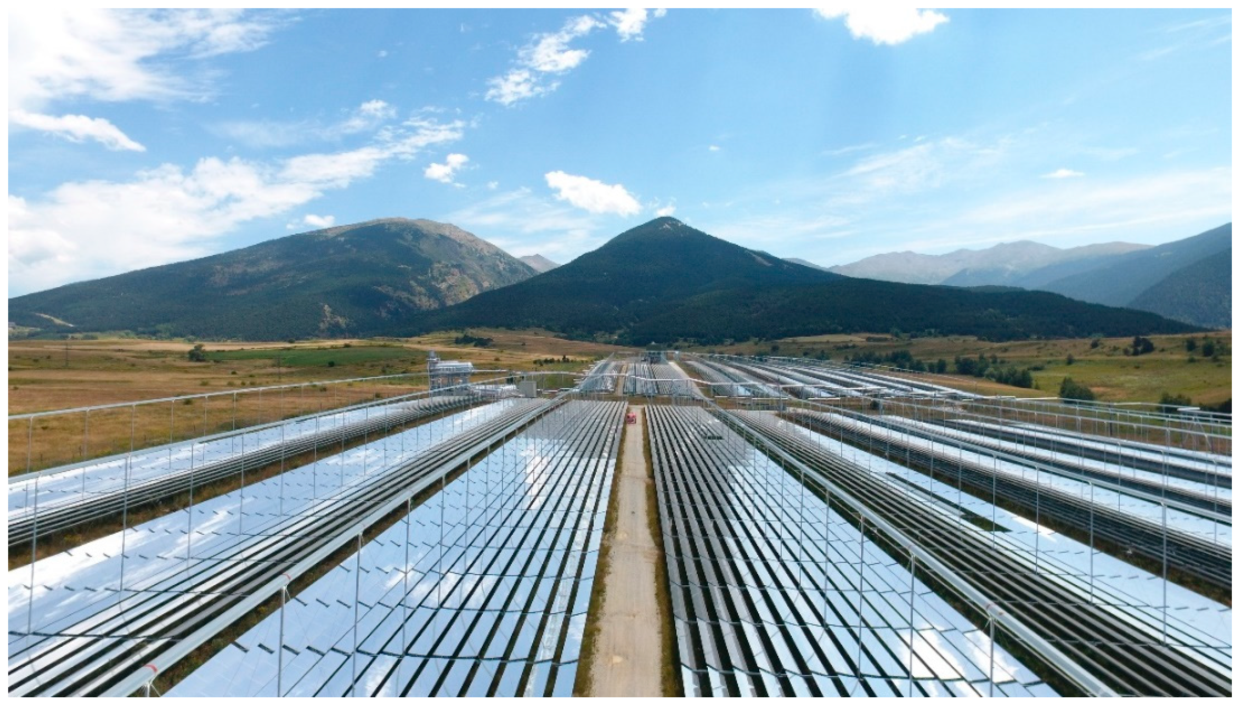
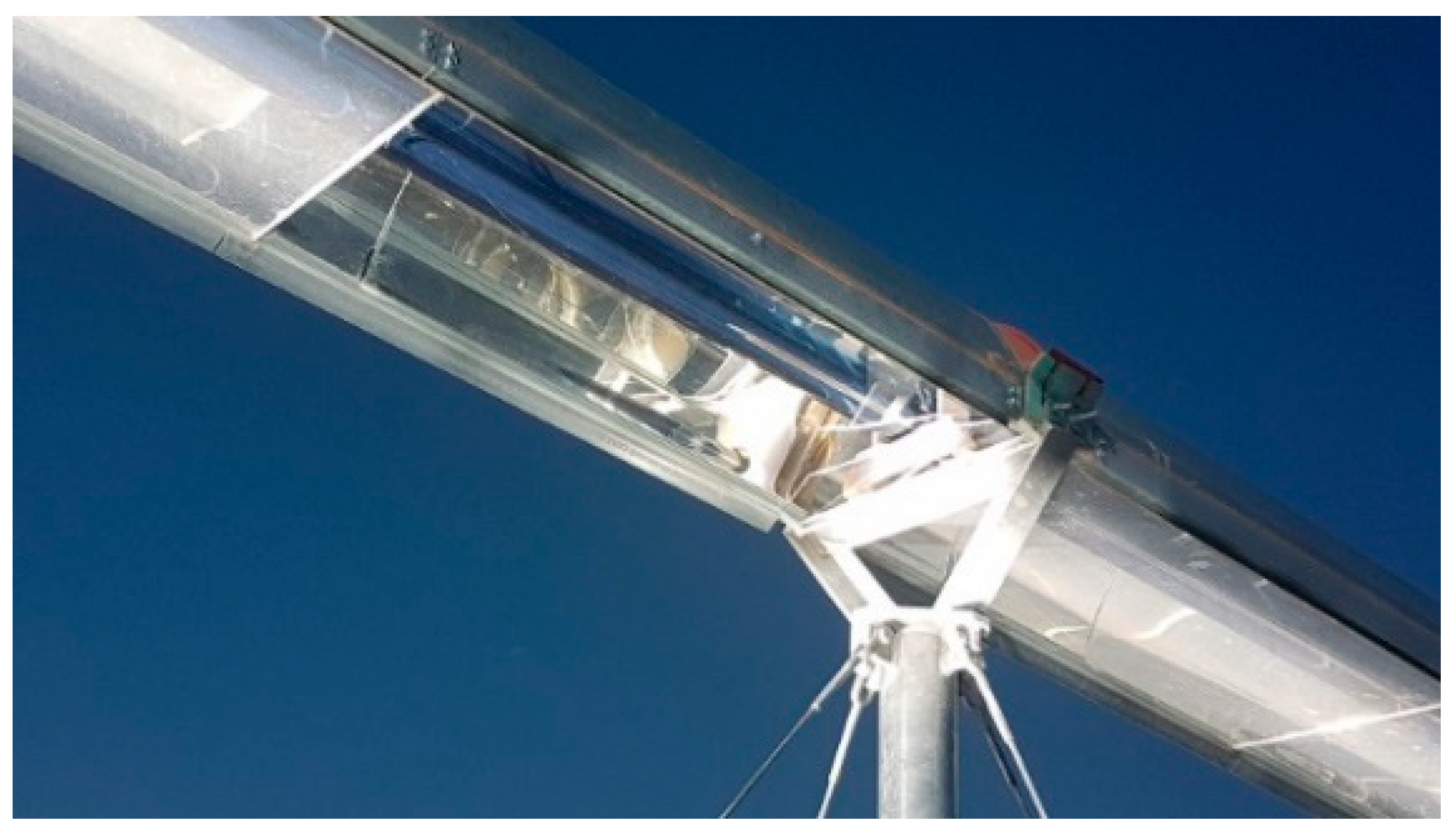
2. eLLO Solar Field Presentation

The eLLO solar power plant, developed by SUNCNIM and operated by eLLO, is located in a hilly terrain in the south of France (42.4662° N; 2.0705° E). It was officially launched in 2019 and is shown in Figure 1. This plant is based on a modular LFC technology, i.e., several modules in series form a solar line and several solar lines in parallel form a solar field. These 67 m long and 18 m wide solar modules are operated for direct steam generation and composed of 27 eLLO solar lines (four- to eight-module long). These lines are oriented with an offset of 50.9° from the NS axis, and the modules are arranged to follow the tilted topography of the site. The eLLO module is equipped with 140 curved primary reflectors (902.2 m2) and a tracking system for both sides of the module that targets the aperture of the solar receiver. This corresponds to a geometric concentration of 48. The solar receiver is installed at 8.5 m above the axes of the mirrors by several guyed masts. The optical efficiency of this system is described in a dedicated article [4] and is equal to 69.5%. Then, separator tanks are used to separate the liquid–steam mixture produced in each solar line; the liquid phase recirculates in the field, and the steam is sent either to the power block or to the storage unit.
Finally, this facility presents specific characteristics considering thermodynamics and optics as the steam storage system, the simplification of the solar tracking system, and the unique solar module configuration adapted to the topographical constraints of the location [4].
The eLLO solar receiver, shown in Figure 2, consists of the following:
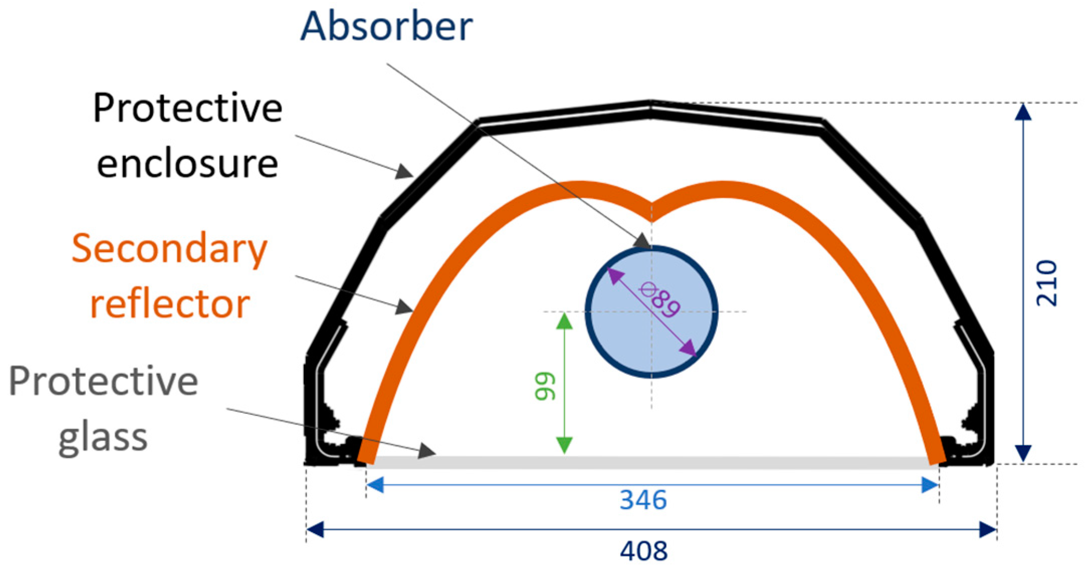
  • A steel absorber tube (1.4301 steel) with a selective coating to enhance the thermo-optical properties;
  • A secondary reflector type compound parabolic concentrator (CPC) made of aluminum, allowing for the reflection of the part of the radiation that does not directly impact the absorber tube;
  • A protective enclosure made of galvanized steel and a specific protective glass to limit convection losses.
Note that the absorber tube is not placed in a vacuum glass envelope, and the cavity between the secondary reflector and the protective enclosure is not insulated.
Table 1 shows the physical and optical properties of the receiver subassemblies.
Each of the solar lines is equipped with a control valve and a Venturi meter at the inlet of each line to regulate and monitor the flow rate through the absorber tube. The water recirculation is ensured by one pump located downstream of the separator tank. This pump has a minimum flow rate of 12 t/h, corresponding to three times the maximum flow rate in a line. Thus, the experimental measurements of heat losses were carried out for a recirculation in three lines minimum to match the pump specifications.
Out of the 27 lines of the power plant, only lines L1, L2 and L3 were fully equipped with PT100 temperature probes at the inlet and outlet of the solar line. This heat loss study is thus carried out on these three instrumented lines, each composed of four modules. The heliostats of these lines were defocused when heat loss experiments were carried out (no solar power input), and the flow rate in each line was between 4 and 5 t/h.

3. Materials and Methods

3.1. Calculation Methods to Evaluate Heat Losses

The heat loss studies of a solar line are evaluated during the water circulation in the absorber in the absence of solar concentration (Figure 3). Thus, the heat balance of the system “absorber tube and fluid” is written as follows:
m a b s × d h a b s d t + m f × d h f d t = m ˙ f × h i n t m ˙ f × h o u t t P l o s s t P s u n e ( t ) ,
where m ˙ f , h i n and h o u t are the flow rate and the inlet/outlet fluid enthalpy, respectively, P l o s s t is the solar receiver heat losses,   m d h d t is the thermal inertia of the absorber tube (abs) and the fluid (f), and P s u n e ( t ) is the incident solar power on the protective enclosure.
When neglecting the solar power on the protective enclosure and considering a steady state, i.e., when the inlet and outlet fluid temperatures are constant, the accumulation terms are null, and Equation (2) simplifies it as follows:
P l o s s , s t e a d y s t a t e t = m ˙ f C p f T i n t T o u t t ,
where T i n ( t ) and T o u t ( t ) are the temperatures at the inlet and outlet of the solar line, and C p f is the fluid heat capacity at the inlet/outlet fluid temperature average.
For the transient state, the calculation method consists in integrating all the terms of the solar receiver heat balance (Equation (1)).
t i t f m a b s × C a b s × d T a b s + t i t f m f × C p f × d T f = t i t f m ˙ f × C p f × T i n t × d t t i t f m ˙ f × C p f × T o u t t × d t t i t f P l o s s t × d t
The absorber tube temperature is assumed to be equal to the inlet/outlet fluid temperature average, and the properties of the fluid are determined for the inlet/outlet fluid temperature average as well.
The main concern of this study is to determine experimentally the heat losses of the receiver without impacting the electricity production of eLLO solar power plant. For this purpose, two protocols were defined depending on the average fluid temperature targeted: the low-temperature protocol for temperature between 50 °C and 150 °C and the high-temperature protocol for temperature between 150 °C and 290 °C.

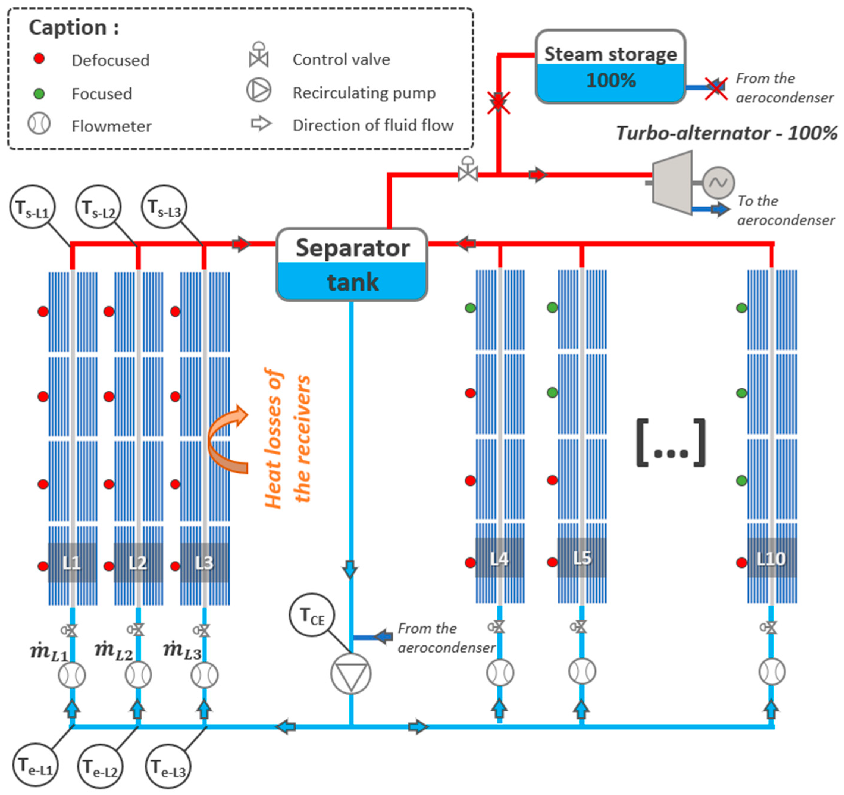
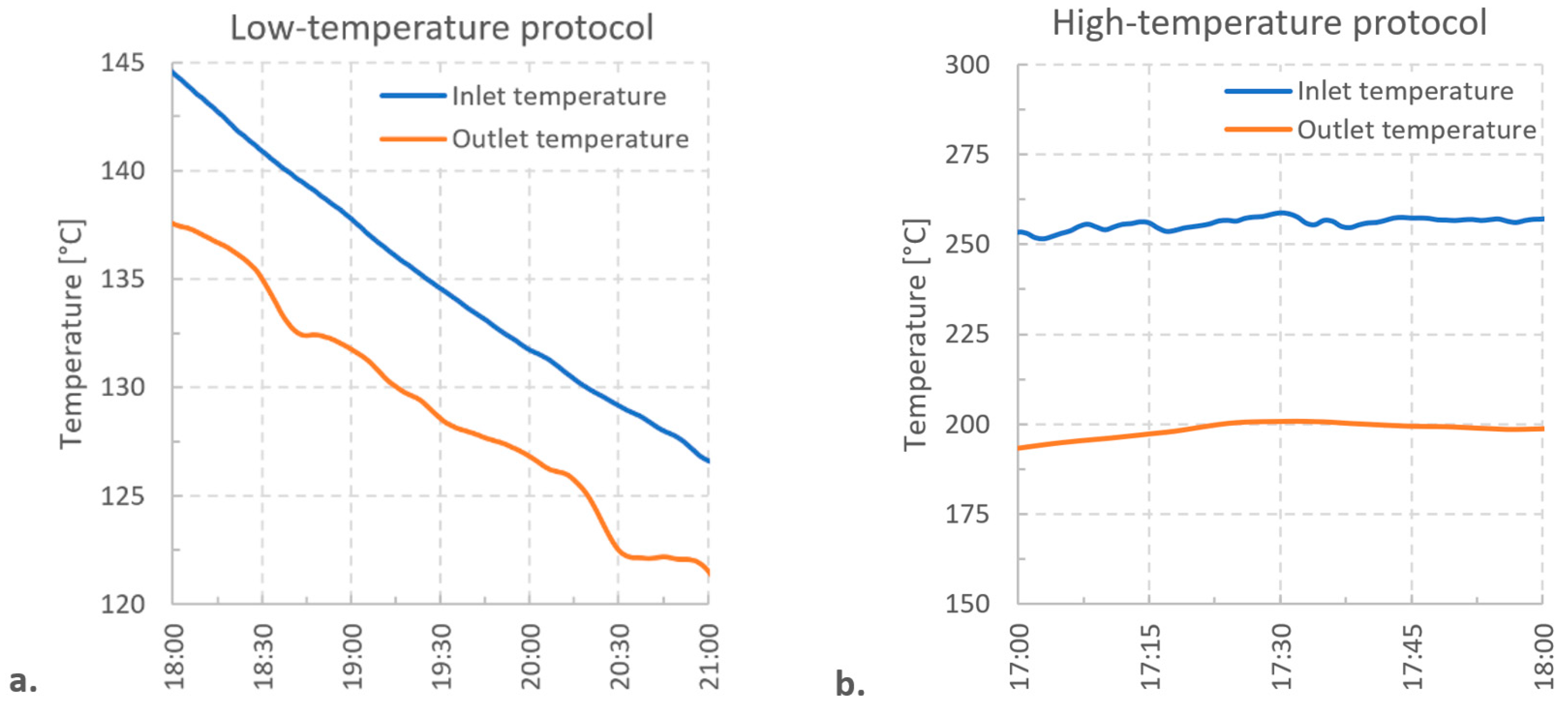
3.2. Low and High-Temperature Protocols

The low-temperature (LT) protocol was operated during the nightly recirculation of the liquid phase from the separator tank to the absorber tubes of the solar field. This operating strategy was implemented after the turbine had stopped, in order to achieve the following:
  • To homogenize the temperatures of the fluid between the solar field and the separator tank and thus limit the water hammer during the restart in summer;
  • To prevent the risk of freezing in winter.
The pressure in the separator tanks was close to the turbine shutdown pressure (7 bars), which corresponds to a saturation temperature of 150 °C. This justifies why this protocol was not suitable for higher fluid temperatures. For the heat loss experiments, the recirculation was restricted to the 3 instrumented lines, as shown in Figure 4, to avoid excessive heat losses from the rest of the solar field and limit the energy loss in the separator tank.
To evaluate the solar receiver heat losses for a fluid temperature higher than 150 °C, the experiments were carried out when the power plant was in operation. To avoid any impact on the production of electrical energy, the high-temperature (HT) protocol studies at high temperature were performed when the turbine was at its nominal operation and the storage system was full. This means a period with excess energy. In this situation, the automation unit controlled the heliostats position to maintain a pressure of 71.5 bar (287.3 °C) in the separator tank by defocusing part of the heliostats so that the solar energy captured compensates the steam extraction to the turbine and the solar field heat losses. Thus, in this case, the heliostats of the 3 instrumented lines were defocused without affecting power generation.
Figure 5 schematizes the control for the high-temperature protocol. Contrary to the low-temperature protocol, the heliostats lines 4 to 10 were partially focused, and the recirculation ensured the extraction of the solar power.

3.3. Temperature Evolution of the Solar Lines

The low and high-temperature protocols are implemented, and the results are presented in Figure 6. Note that in the following section, the measurements correspond to the average of the measurements on lines L1, L2 and L3. The graphs as a function of time are expressed as Universal Coordinated Time UTC+1 in winter and UTC+2 in summer.
In the case of the low-temperature protocol (winter), the inlet temperature decreases linearly as well as the outlet temperature. For the high-temperature protocol (summer), the inlet temperature admits a maximum variation of 7.2 °C for this case. Thus, for the two cases, the steady state was not exactly reached.

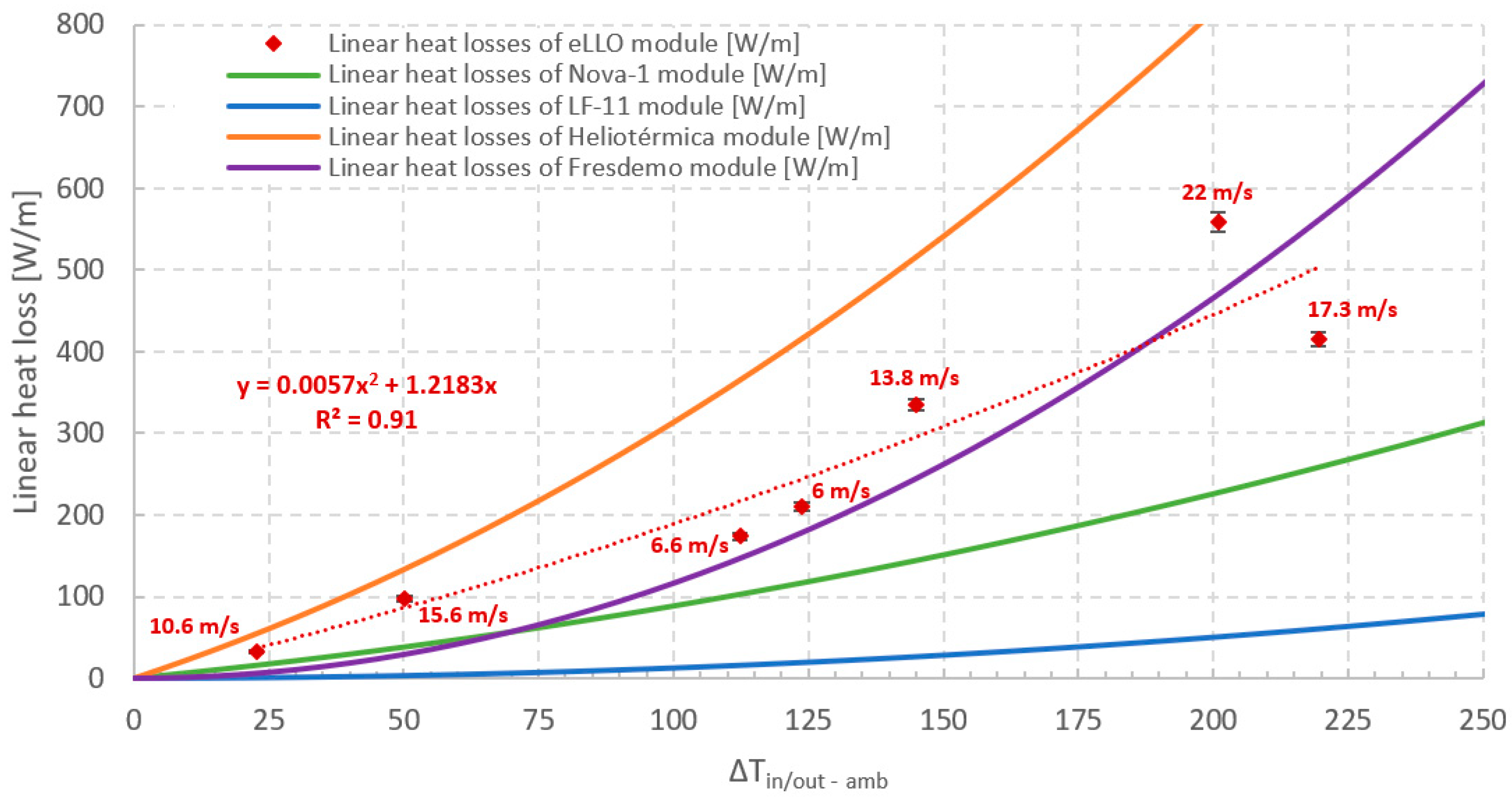
4. Empirical Heat Loss Correlation of the eLLO Receiver

The two protocols were implemented multiple times to determine the receiver heat losses for the seven cases shown in Table 2. The maximum inlet temperature variation is the difference between the maximum and minimum inlet temperatures in the study interval.
The difference between the inlet/outlet fluid temperature average and the ambient temperature are in the ranges of the low-temperature and high-temperature protocol. For the LT protocol, the 1.1 kg/s flow rate in the three lines corresponds to the pump minimum flow rate. As shown in the previous paragraph, the variation in the inlet temperature does not allow achieving an exact steady state. For the LT protocol, the maximum variations in the inlet temperature are higher than 9 °C, except for 13/01/2023. For the HT protocol, the maximum variation in the inlet temperature is lower than the maximum variation for the LT protocol but still too large to be considered as a steady state.
Figure 7 presents the experimental heat loss correlation as a function of the difference between the inlet/outlet fluid temperature average and the ambient temperature. Then, this correlation is compared to the heat loss correlation described by other solar modules’ manufacturers, Frenell, Industrial Solar, LEPTEN laboratory and Ciemat named Nova-1, LF-11, Heliotérmica and Fresdemo, respectively. Table 3 shows some of the geometric specifications of the compared modules. The experimental heat losses as well as the heat losses evaluated using the manufacturers’ data are expressed in terms of heat loss divided by the length of the studied system. They refer to linear heat losses that enable direct comparisons between the different Fresnel manufacturing designs [25,27,31,32].
The calculation uncertainty is evaluated based on the measurement uncertainties of the PT100 probes and flowmeters. The measurement uncertainty of the orifice meter is considered to be equal to 0.5% [33], and the measurement uncertainty of the PT100 probes is equal to ±0.2 °C [34].
The experimental heat losses are obtained for different wind conditions as shown in the Figure 7. The cases with low wind speeds are close to Fresdemo’s heat losses, while the cases with higher wind speeds generally have heat losses between the linear heat losses of the Heliotérmica receiver and the Fresdemo receiver.
The heat loss of the eLLO module is equal to 311 W/m under the following reference conditions: 175 °C inlet/outlet fluid temperature average, 25 °C ambient temperature. For the same condition, the heat loss of the Fresdemo facility is equal to 262 W/m. As the receiver architecture is almost identical, the higher heat losses of the eLLO module can be explained by the presence of insulation behind the secondary reflector in the Fresdemo receiver but also by the missing glasses and the tilted receiver in the eLLO plant.
Note that the very low linear heat losses of the LF-11 module are due to the vacuum tube surrounding the absorber tube, limiting the convective heat losses of the system.
Indeed, the eLLO receiver conditions and, in particular, when some of the protective glasses were missing (Figure 8), led to a strong dependence of heat losses on wind condition. Table 4 presents the number of missing glasses and the ratio between the number of missing glasses and the total number of glasses of the receiver (320 glasses for a 268 m long receiver) of the three instrumented lines visually recorded on 08/07/2022.
Thus, the disparity in the results expressed by the R2 = 0.91 shows the strong dependence of heat losses on wind conditions. However, due to the few experimental points and because the local wind conditions are not precisely monitored along the entire lines (a single weather station for the entire site), it is difficult to define an empirical functional relation with wind conditions. Thus, a 1D single-phase thermohydraulic model based on MATLAB is developed to express theoretical heat loss correlations, however, limiting it to the influence of the wind speed for the sake of simplicity.
Finally, an empirical correlation of the linear heat losses of the eLLO receiver is expressed in Equation (4) as a second-degree polynomial according to the difference between the inlet/outlet fluid temperature average and the ambient temperature.
P l o s s e L L O = 5.7 10 3 T m e a n T a m b 2 + 1.2193   T m e a n T a m b
This correlation is compared in the following section with the numerical correlation expressed using the 1D single-phase thermohydraulic model.

5. Single-Phase Thermohydraulic Model

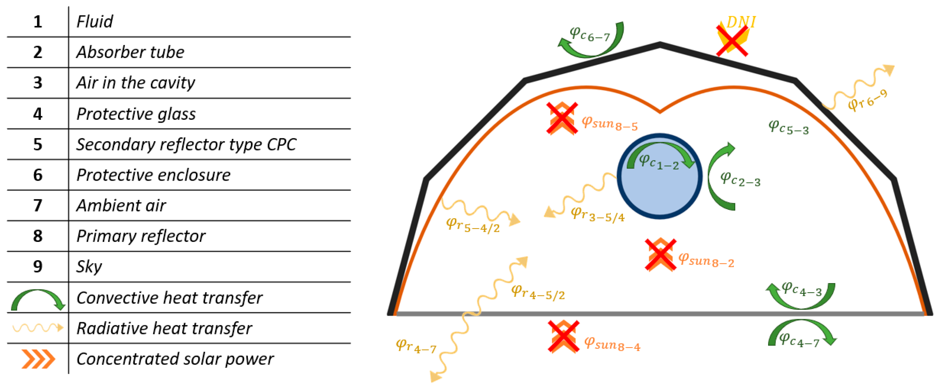
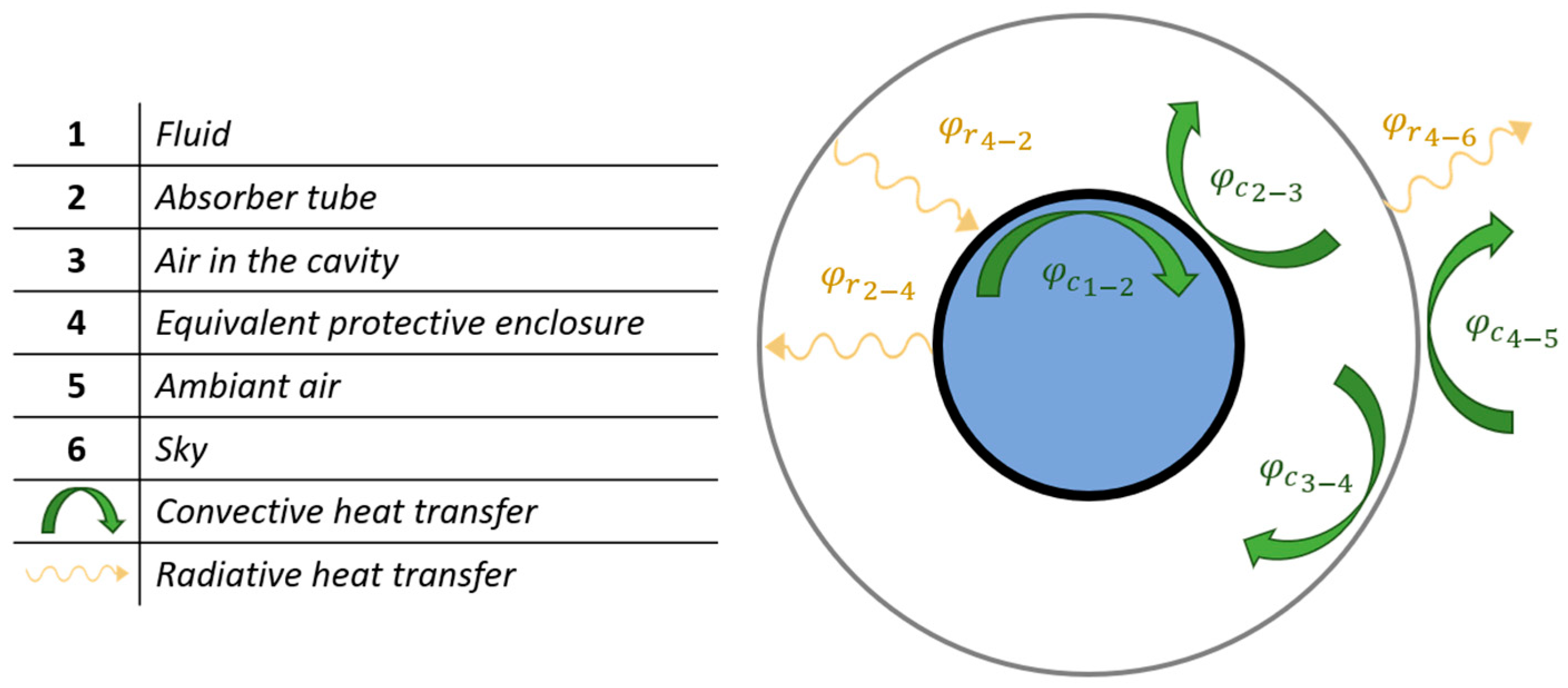
5.1. Model Hypothesis and Physical Equations

The 1D single-phase thermohydraulic model is adapted from the work of Fasquelle et al. [35] describing the thermo-optical performance of a parabolic trough concentrator equipped with a vacuum absorber tube. In our case, the objective is to simulate the single-phase flow in the absorber tube as well as the thermal exchange involved in the receiver.
Figure 9 shows the eLLO solar receiver architecture composed of an absorber tube, a secondary reflector type CPC and the protective enclosure. The subassemblies of the receiver are numbered to express the radiative and convective transfers between the elements of the eLLO solar receiver. For example, the protective glass (4) exchanges radiative heat with both the absorber tube (2) and the CPC (5) expressed as φ_(4 − 5/2). Finally, conduction heat transfer in the thickness of materials and in air as well as solar power directly impacting the receiver are neglected. At last, the protocols is designed to ensure that there is no concentrated solar flux at the receiver during measurements.
The complex geometry of the receiver is simplified and approximated by two coaxial tubes, one representing the absorber tube and the other the equivalent protective enclosure (enclosure + protective glass) (Figure 10). Equation (5) is used to evaluate the diameter of this equivalent protective enclosure so that its surface is equivalent to the surface of the enclosure and the protective glass of the eLLO receiver.
D e q o u t = π D e n o u t 2 + l v × L c π × L c = 0.334   m
where D e n is the protective enclosure diameter, l v is the width of the receiver aperture, and L c is the length of the collector.
Figure 10 shows the simplified geometry and the heat transfers involved.
The following assumptions are made to simplify the resolution of the calculations:
  • The glass, the secondary reflector and the protective enclosure are considered as a single body exchanging heat with the absorber tube and the environment. The physical and optical properties of the equivalent protective enclosure are approximated by the average of the properties shown in Table 1.
  • The thermal properties of the absorber and the envelope are constant for the considered temperatures.
  • The radiation between the absorber tube and the protective enclosure is considered between two concentric semi-infinite tubes.
  • The protective enclosure radiates towards a virtual environment at a sky temperature assumed to be 8 °C lower than the ambient temperature [36].
  • The velocity of the heat transfer fluid and the temperature are considered uniform over the tube section.
  • The thermal diffusion along the tube axis is considered.
  • Only the continuity equation is solved to conserve mass as the fluid heats up. Other fluid mechanics considerations are not considered.
  • The absorber tube is supported on the guyed masts by a plastic pulley, the conductive heat loss through this support is neglected.
  • The heat loss on short pipe runs at the inlet and outlet solar line is neglected.
The simulations are performed for a 268 m long receiver, corresponding to the length of each of the three instrumented lines. The temperature and pressure along the absorber tube are initialized by considering a linear evolution of the temperature and pressure between the inlet and the outlet. The initial temperature of the absorber is determined as being equal to the fluid temperature, and the initial temperature of the protective enclosure is imposed as being equal to the outside temperature.
The energy conservation equations applied to each subset are as follows:
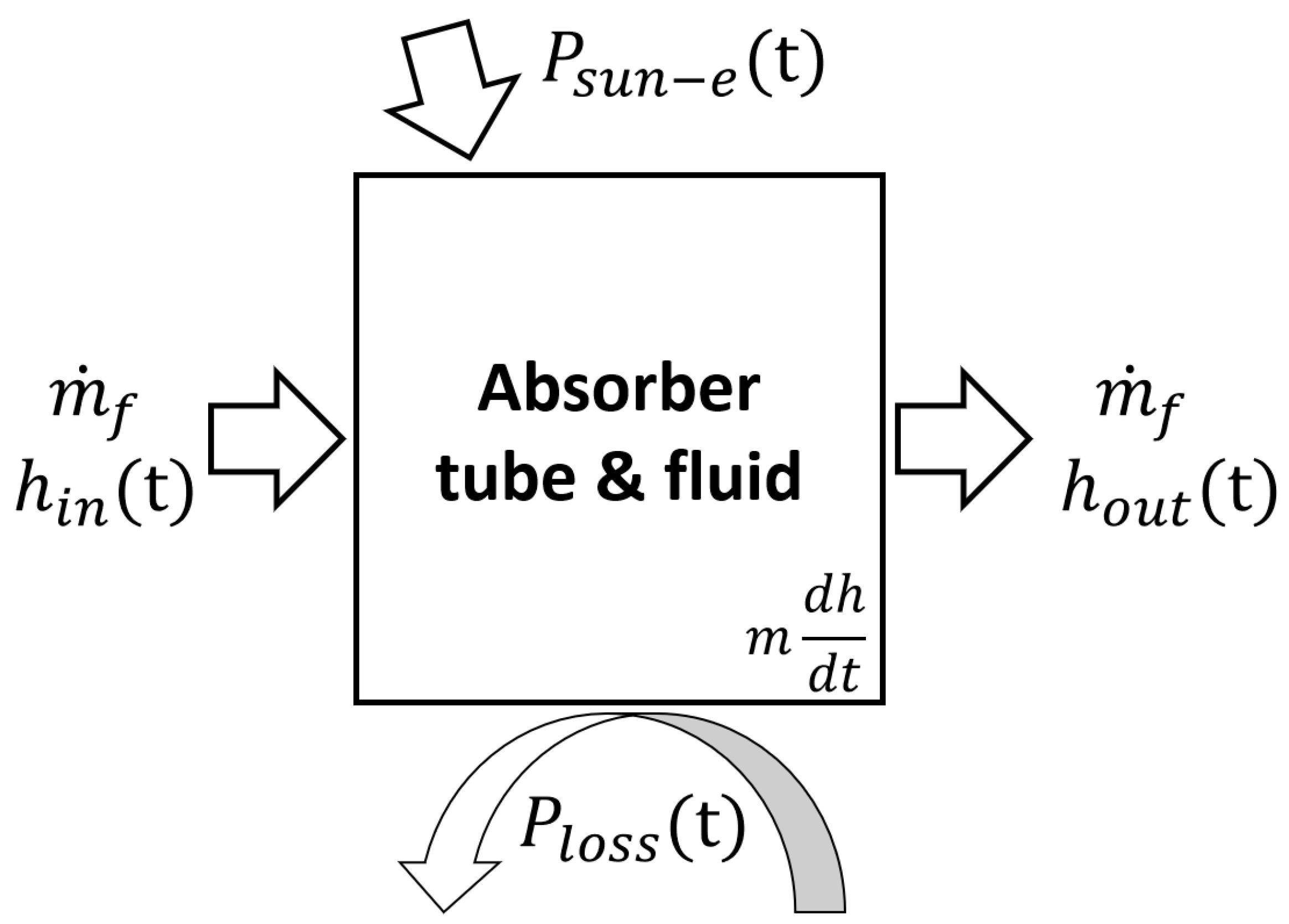
  • The energy conservation equation of the heat transfer fluid contains an accumulation term, an axial diffusion term, an advective term and a convective exchange term with the absorber tube (Equation (6)):
h f t = Γ f ρ f × 2 h f x 2 U f × h f x + D a b s i n ρ f × A   a b s i n × φ c o n v
where Γ f , ρ f and h f are the thermal diffusivity, the density and the enthalpy of the fluid, respectively, U f is the velocity of the fluid in the absorber tube, and φ c o n v is the heat flux density exchanged between the fluid and the wall.
  • The energy conservation equation of the absorber tube contains an accumulation term, an axial diffusion term, two convective exchange terms, one with the transfer fluid and the other with the air in the cavity and a radiation term with the protective enclosure:
T a b s t = λ a b s ρ C a b s × 2 T a b s x 2 h c a v × D a b s o u t ρ C a b s × A a b s o u t × T a b s T c a v i t y h f × D a b s i n ρ C a b s × A a b s i n × T a b s T f + B e n a b s × D a b s o u t ρ C a b s × A a b s o u t × σ × T a b s 4 T e n 4
where   B e n a b s = 1 ε a b s + 1 ε e n ε e n × D a b s o u t D e q i n 1
where λ a b s is the thermal conductivity of the absorber steel, T c a v i t y is the temperature of the air in the cavity equal to the average temperature of the absorber and the protective enclosure, h c a v is the convective heat transfer coefficient in the cavity, and, finally, ε a b s and ε e n are the emissivity of the absorber tube and of the equivalent protective enclosure, respectively.
  • The energy conservation equation of the protective enclosure contains an accumulation term, an axial diffusion term, two convection terms, one with the cavity air and the other with the outside and two radiation terms, one with the absorber tube and the other with the sky:
T e n t = λ e n ρ C e n × 2 T e n x 2 h o u t × D e q o u t ρ C e n × A e q o u t × T e n T a m b h c a v × D e q i n ρ C e n × A e q i n × T e n T c a v i t y ε e n × σ × D e q o u t ρ C e n × A e q o u t × T e n 4 T s k y 4 B e n v a b s × D e q i n ρ C e n × A e q i n × σ × T e n 4 T a b s 4
where h o u t is the convective heat transfer coefficient at the outside of the equivalent protective enclosure, and T a m b is the ambient temperature.
  • The convective exchanges are determined using correlations constraining convective heat transfer coefficient. The Nusselt number, Equation (10), reflects the quality of the heat exchange and allows finding the convective exchange coefficients. Each correlation was found in [37], and the condition of application was verified.
N u = h L c λ f
  • The convective heat transfer within the absorber tube is described by the correlation of Dittus and Boelter. Equation (11) introduces the Dittus and Boelter correlation in the case where the wall temperature is colder than the fluid temperature:
N u D = 0.0265   R e D 0.8 P r 0.3  
where R e L is the Reynolds number, and P r is the Prandtl number.
  • The convective heat transfer within the cavity is assumed to be a natural convective exchange, described by the Mac Adams correlation (Equation (12)):
N u D = 0.13   R a D 1 / 3
where R a L = g × c o s θ × β × ( T a b s T c a v ) × D e q o u t 3 α   v ,   g is the gravitation constant, β is the coefficient of expansion of the fluid, θ is the slope of the system in the longitudinal plane, α is the thermal diffusivity of the fluid, and v is the dynamic viscosity of the fluid.
  • The convective heat transfer between the enclosure and the environment differs according to the wind speed. If the wind speed is less than 1 m/s, then a natural convective heat transfer correlation around a horizontal cylinder is chosen (Equation (13)). Otherwise, the heat transfer coefficient is determined using the Hilpert correlation describing convective heat transfer for flows around a cylinder (Equation (14)). The characteristic length corresponds to the external diameter of the protective enclosure.
  • If V w i n d < 1   m / s ,
    N u D = 0.53   R a D 1 / 4                         i f   R a D 10 3 ; 10 9 N u D = 0.10   R a D 1 / 3                         i f   R a D 10 9 ; 10 13
  • In addition,
N u D = 0.43 + 0.53   R e D 0.5   P r 0.31 i f   R e D 1 ;   4000 N u D = 0.43 + 0.193   R e D 0.618   P r 0.31 i f   R e D 4000 ;   40000 N u D = 0.43 + 0.0265   R e D 0.805   P r 0.31 i f   R e D 40000 ;   400000
The single-phase model is fed by experimental measurements of the temperature and pressure at the line inlet, the mass flow rate, the average outdoor temperature over the study interval as well as the wind speed at the receiver. The equations are solved using the finite difference method with an implicit temporal discretization and a spatial discretization along the receiver. The time step is equal to 1 s, and the spatial discretization is 1 m. The fluid enthalpy vector, the absorber tube temperature vector and the equivalent protective enclosure temperature vector are found iteratively, with a convergence criterion of 10−4, for each time step using the MATLAB software (R2020a version).

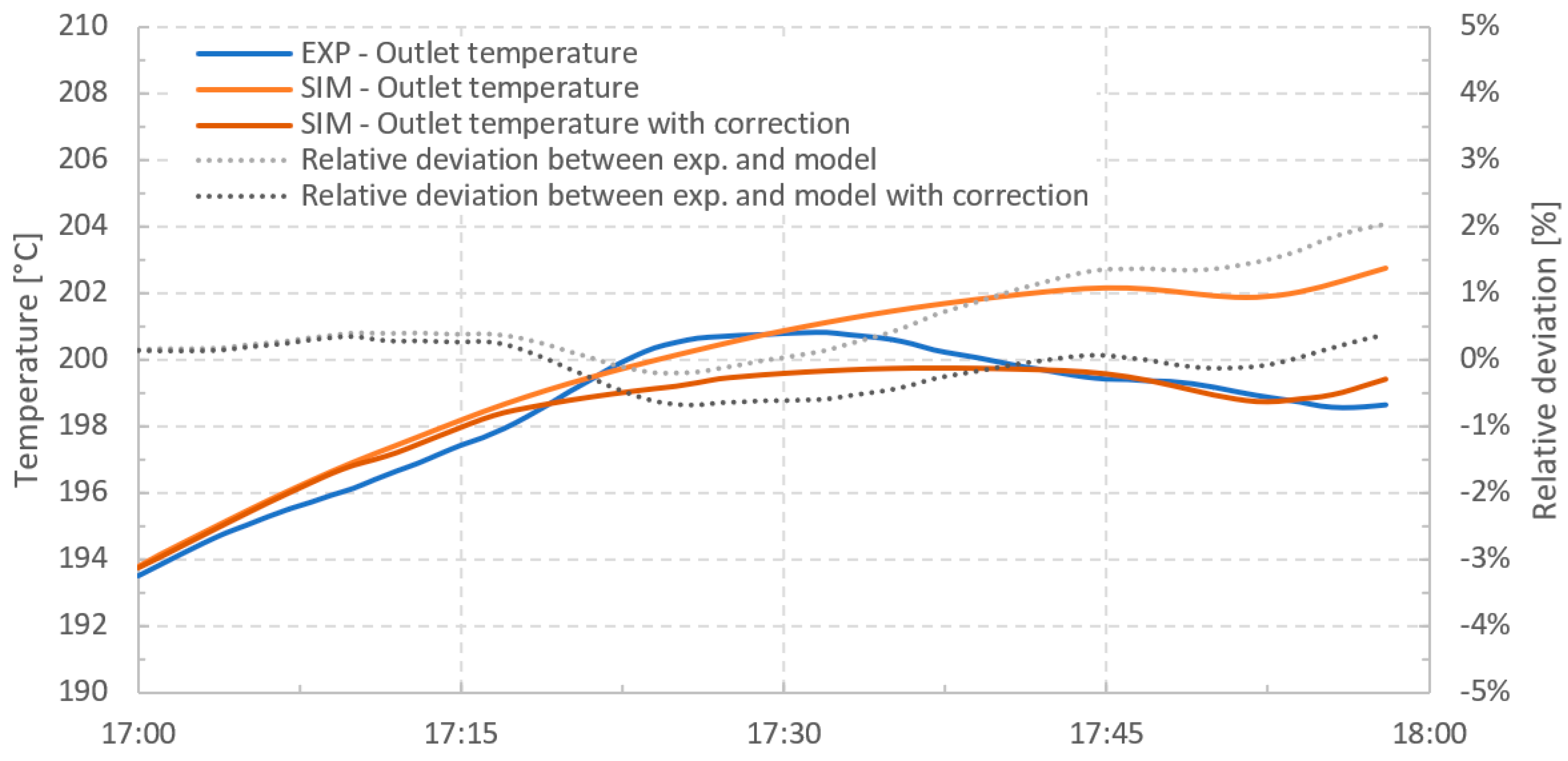
5.2. Validation and Improvement of the Single-Phase Model

The validation of the single-phase thermohydraulic model is realized by comparing the theoretical and experimental outlet temperatures. The experimental data, expressed in Table 2, are used as model input data. Figure 11 shows the experimental outlet temperature and the theoretical outlet temperature of the single-phase thermohydraulic model for 01/07/2022.
The output temperature of the single-phase model followed the evolution of the experimental temperature with a relative deviation lower than 1% before 17:20, and then the relative deviation increased to reach 2.1% at 18:00. At first glance, the disparity between the experimental results and the model seems to be related to the increase in the wind speed at 17:20. Thus, the model underestimated the heat losses for the wind speed higher than 15 m/s.
As shown in Section 4, the solar receiver partially degraded conditions led to an increase in the receiver heat losses with the wind conditions. To account for the protective glass missing, the assumption of natural convective heat transfer in the cavity was modified. The complex geometry coupled with the uneven condition of the receivers make the use of forced convection correlations from the literature inadequate. Instead, a correction was applied for the natural convective heat transfer in the cavity according to the wind speed for each step, such that:
h c a v = N u L × λ c a v L c ,           i f   V w i n d < 15   m / s h c a v = 1.15 × N u L × λ c a v L c ,           i f   V w i n d > 15   m / s
The correction coefficient of Equation (15) is chosen such as to minimize the relative difference between the experimental and theoretical outlet temperature for the data of 01/07/2022. Figure 12 shows the evolution of the experimental and simulated outlet temperature with and without the correction coefficient for the natural convective heat transfer in the cavity.
With the correction, the maximum absolute relative deviation between the experimental data and the simulated results is equal to 0.7%, by comparison without the correction, the maximum relative deviation is equal to 2.1%. Thus, the correction for the heat exchange coefficient in the cavity allows improving the results of the model by reducing the relative deviation between the outlet temperatures.
Table 5 presents the influence of the correction on the maximum relative deviation between the experimental and theoretical outlet temperatures for the 7 experimental days.
For all cases, the correction allows decreasing the maximum relative deviation between the experimental and simulated output temperatures except for the cases where wind speeds do not exceed 15 m/s over the study interval (14/06/2022 and 06/09/2022) since in this case, the calculation is not modified. Note that the wind speed is averaged over the study interval, and the effect of the correction is visible in the case of 13/01/2023, since the wind speed occasionally exceeds 15 m/s.
To assess the model accuracy, the theoretical results, obtained with the same initial condition and input data as in the experimental study (Table 2), are expressed as a function of the experimental results in a parity plot on Figure 13 (including a 10%, 20% and 30% deviation).
The resulting points are almost exclusively included in the ±30% deviation domain, except for 27/09/2022 with a low-temperature study and high wind speed condition with a deviation slightly higher than −30%.
Thus, the single-phase thermohydraulic model allows the experimental heat losses to be evaluated within a reasonable uncertainty of ±30% regardless of the wind velocity. Henceforth, the model is used to express the receiver heat losses for different inlet fluid temperatures and wind speeds.

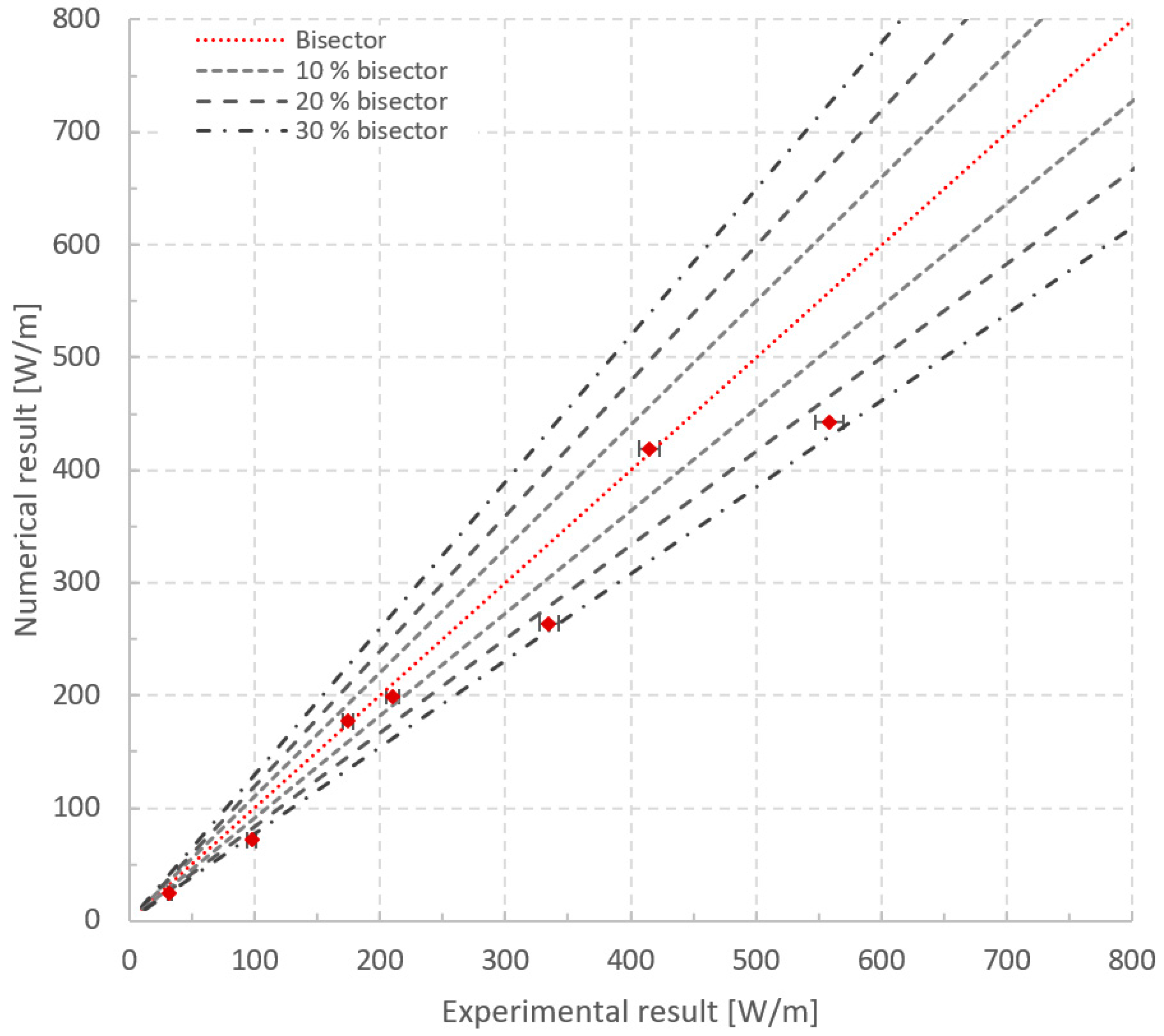
5.3. Numerical Heat Loss Correlation Depending on Wind Speed

To express the receiver heat losses according to the wind speed, the single-phase thermohydraulic model is used to determine heat loss correlation for the wind speed equal to 0 m/s, 10 m/s and 20 m/s and the inlet temperature from 50 °C to 250 °C with 50 °C steps.
Figure 14 shows the experimental linear heat losses and the theoretical linear heat losses as a function of the difference between the average inlet/outlet fluid temperature and the ambient temperature. The experimental points are labeled with the average wind speed and expressed with the measurement uncertainty.
First, the single-phase thermohydraulic model is compared to the thermal model, presented by Mertins [38], for the thermal losses from a receiver as a function of the outer absorber diameter and the absorber emittance. The difference between the Mertins model and the eLLO theoretical heat losses for a 0 m/s wind speed is explain by the high heat transfer coefficient in the cavity in the case of the tilted and somehow degraded (missing glasses) eLLO receiver.
As for the experimental heat loss correlation, the three theoretical linear heat loss correlations are expressed as second-degree polynomials in (Equations (16)–(18)):
P l o s s 0   m / s = 2.8 × 10 3 T m e a n T a m b 2 + 0.9961   T m e a n T a m b
P l o s s 10   m / s = 3.4 × 10 3 T m e a n T a m b 2 + 1.2169   T m e a n T a m b
P l o s s 20   m / s = 3.8 × 10 3 T m e a n T a m b 2 + 1.3932   T m e a n T a m b
Therefore, some of the experimental results are in good accordance with the theoretical ones. For example, the results of 01/07/2022 with an averaged wind speed equal to 21.6 m/s but with the wind speed below 15 m/s at the start of the study interval.
The comparison shows that the single-phase thermohydraulic model can be used to determine heat losses from the eLLO receiver as a function of wind speed with varying degrees of accuracy.

6. Conclusions

The study of the eLLO receiver heat losses was carried out on three instrumented lines of the operating power plant. This study was constrained by the commercial electricity production of the plant. Thus, two experimental protocols were operated to evaluate the receiver heat losses, over a wide range of fluid temperatures, without impacting the plant operation.
First, the eLLO receiver heat losses were determined experimentally by applying both protocols. An empirical heat loss correlation is defined as a second-degree polynomial and is compared to other LFC receiver heat loss correlations. The eLLO heat loss correlation is between the heat loss correlations of the Heliotérmica receiver and the Fresdemo receiver. The heat loss of the eLLO module is equal to 311 W/m under the following reference conditions: 175 °C inlet/outlet fluid temperature average, 25 °C ambient temperature, no wind. This heat loss is higher than the one observed on the Fresdemo facility under the same reference conditions due to the slope of the eLLO receiver and the absence of some protective glasses. The significant disparity in the experimental results can be attributed to the strong influence of the wind speed on heat losses. Nevertheless, the limited number of experimental data points was inadequate for representing distinct correlations based on the wind speed. For this purpose, a 1D single-phase thermohydraulic model was developed and adapted to the receiver’s current condition (missing glasses). This model is validated by comparing it with the model proposed by Mertins and by comparing the experimental results. This comparison indicates that the model can effectively estimate receiver heat losses with an acceptable uncertainty of approximately ±30%, regardless of the wind velocity.

Author Contributions

Writing—original draft preparation, E.M.; writing—review and editing, E.M., S.R., Q.F. and F.R.; supervision, S.R. and Q.F.; project administration, S.R. and Q.F.; funding acquisition, Q.F. All authors have read and agreed to the published version of the manuscript.

Funding

This work was supported by the program “Investissements d’Avenir” Labex Solstice managed by the National Research Agency (ANR-10-LABX-22-01) and by the National Agency for Technological Research (CIFRE contract n° 2020/0451, 2021).

Data Availability Statement

Data are contained within the article.

Acknowledgments

The authors thank Christophe Escape (PROMES-CNRS; PCM-OPT) for the optical characterization of the eLLO absorber tube.

Conflicts of Interest

F.R. and E.M. are employees of eLLO company. The other authors declare no conflict of interest.

References

  1. Papadis, E.; Tsatsaronis, G. Challenges in the Decarbonization of the Energy Sector. Energy 2020, 205, 118025. [Google Scholar] [CrossRef]
  2. Baharoon, D.A.; Rahman, H.A.; Omar, W.Z.W.; Fadhl, S.O. Historical Development of Concentrating Solar Power Technologies to Generate Clean Electricity Efficiently—A Review. Renew. Sustain. Energy Rev. 2015, 41, 996–1027. [Google Scholar] [CrossRef]
  3. Abbas, R.; Muñoz-Antón, J.; Valdés, M.; Martínez-Val, J.M. High Concentration Linear Fresnel Reflectors. Energy Convers. Manag. 2013, 72, 60–68. [Google Scholar] [CrossRef]
  4. Montanet, E.; Rodat, S.; Falcoz, Q.; Roget, F. Influence of Topography on the Optical Performances of a Fresnel Linear Asymmetrical Concentrator Array: The Case of the ELLO Solar Power Plant. Energy 2023, 274, 127310. [Google Scholar] [CrossRef]
  5. Montenon, A.C.; Santos, A.V.; Collares-Pereira, M.; Montagnino, F.M.; Garofalo, R.; Papanicolas, C. Optical Performance Comparison of Two Receiver Configurations for Medium Temperature Linear Fresnel Collectors. Sol. Energy 2022, 240, 225–236. [Google Scholar] [CrossRef]
  6. Balaji, S.; Reddy, K.S.; Sundararajan, T. Optical Modelling and Performance Analysis of a Solar LFR Receiver System with Parabolic and Involute Secondary Reflectors. Appl. Energy 2016, 179, 1138–1151. [Google Scholar] [CrossRef]
  7. Mills, D.R. Linear Fresnel Reflector (LFR) Technology. In Concentrating Solar Power Technology; Woodhead Publishing: Cambridge, UK, 2012; pp. 153–196. [Google Scholar]
  8. Abbas, R.; Martínez-Val, J.M. Analytic Optical Design of Linear Fresnel Collectors with Variable Widths and Shifts of Mirrors. Renew. Energy 2015, 75, 81–92. [Google Scholar] [CrossRef]
  9. Mathur, S.S.; Kandpal, T.C.; Negi, B.S. Optical Design and Concentration Characteristics of Linear Fresnel Reflector Solar Concentrators—II. Mirror Elements of Equal Width. Energy Convers. Manag. 1991, 31, 221–232. [Google Scholar]
  10. Jafrancesco, D.; Cardoso, J.P.; Mutuberria, A.; Leonardi, E.; Les, I.; Sansoni, P.; Francini, F.; Fontani, D. Optical Simulation of a Central Receiver System: Comparison of Different Software Tools. Renew. Sustain. Energy Rev. 2018, 94, 792–803. [Google Scholar] [CrossRef]
  11. Facão, J.; Oliveira, A.C. Numerical Simulation of a Trapezoidal Cavity Receiver for a Linear Fresnel Solar Collector Concentrator. Renew. Energy 2011, 36, 90–96. [Google Scholar] [CrossRef]
  12. López-Alvarez, J.A.; Larraneta, M.; Silva-Pérez, M.A.; Lillo-Bravo, I. Impact of the Variation of the Receiver Glass Envelope Transmittance as a Function of the Incidence Angle in the Performance of a Linear Fresnel Collector. Renew. Energy 2020, 150, 607–615. [Google Scholar] [CrossRef]
  13. Beltagy, H. A Secondary Reflector Geometry Optimization of a Fresnel Type Solar Concentrator. Energy Convers. Manag. 2023, 284, 116974. [Google Scholar] [CrossRef]
  14. Singh, P.L.; Sarviya, R.M.; Bhagoria, J.L. Heat Loss Study of Trapezoidal Cavity Absorbers for Linear Solar Concentrating Collector. Energy Convers. Manag. 2010, 51, 329–337. [Google Scholar] [CrossRef]
  15. Reynolds, D.J.; Jance, M.J.; Behnia, M.; Morrison, G.L. An Experimental and Computational Study of the Heat Loss Characteristics of a Trapezoidal Cavity Absorber. Sol. Energy 2004, 76, 229–234. [Google Scholar] [CrossRef]
  16. Ardekani, M.M.; Craig, K.J.; Meyer, J.P. Combined Thermal, Optical and Economic Optimization of a Linear Fresnel Collector. AIP Conf. Proc. 2017, 1850, 040004. [Google Scholar]
  17. Pye, J.D.; Graham, M.L.; Behnia, M.; Mills, D.R. Modelling of Cavity Receiver Heat Transfer for the Compact Linear Fresnel Reflector. In Paper Knowledge: Toward a Media History of Documents; Duke University Press: Durham, NC, USA, 2014. [Google Scholar]
  18. Tian, M.; Su, Y.; Zheng, H.; Pei, G.; Li, G.; Riffat, S. A Review on the Recent Research Progress in the Compound Parabolic Concentrator (CPC) for Solar Energy Applications. Renew. Sustain. Energy Rev. 2018, 82, 1272–1296. [Google Scholar] [CrossRef]
  19. Qiu, Y.; He, Y.L.; Wu, M.; Zheng, Z.J. A Comprehensive Model for Optical and Thermal Characterization of a Linear Fresnel Solar Reflector with a Trapezoidal Cavity Receiver. Renew. Energy 2016, 97, 129–144. [Google Scholar] [CrossRef]
  20. Abbas, R.; Martínez-Val, J.M. A Comprehensive Optical Characterization of Linear Fresnel Collectors by Means of an Analytic Study. Appl. Energy 2017, 185, 1136–1151. [Google Scholar] [CrossRef]
  21. Babu, M.; Kuzmin, A.M.; Babu, P.S.; Raj, S.S.; Thiruvasagam, C. Angular Error Correction and Performance Analysis of Linear Fresnel Reflector Solar Concentrating System with Varying Width Mirror Reflector. Mater. Today Proc. 2021, 45, 2348–2353. [Google Scholar] [CrossRef]
  22. Zhu, G. Development of an Analytical Optical Method for Linear Fresnel Collectors. Sol. Energy 2013, 94, 240–252. [Google Scholar] [CrossRef]
  23. Chaitanya Prasad, G.S.; Reddy, K.S.; Sundararajan, T. Optimization of Solar Linear Fresnel Reflector System with Secondary Concentrator for Uniform Flux Distribution over Absorber Tube. Sol. Energy 2017, 150, 1–12. [Google Scholar] [CrossRef]
  24. Beltagy, H.; Semmar, D.; Lehaut, C.; Said, N. Theoretical and Experimental Performance Analysis of a Fresnel Type Solar Concentrator. Renew. Energy 2017, 101, 782–793. [Google Scholar] [CrossRef]
  25. Montes, M.J.; Barbero, R.; Abbas, R.; Rovira, A. Performance Model and Thermal Comparison of Different Alternatives for the Fresnel Single-Tube Receiver. Appl. Therm. Eng. 2016, 104, 162–175. [Google Scholar] [CrossRef]
  26. Montenon, A.C.; Tsekouras, P.; Tzivanidis, C.; Bibron, M.; Papanicolas, C. Thermo-Optical Modelling of the Linear Fresnel Collector at the Cyprus Institute. AIP Conf. Proc. 2019, 2126, 100004. [Google Scholar]
  27. Bittencourt de Sá, A.; Pigozzo Filho, V.C.; Tadrist, L.; Passos, J.C. Experimental Study of a Linear Fresnel Concentrator: A New Procedure for Optical and Heat Losses Characterization. Energy 2021, 232, 121019. [Google Scholar] [CrossRef]
  28. Lamineries MATTHEY, Acier 1.4301. Available online: https://www.matthey.ch/alliages/aciers-inoxydables (accessed on 3 May 2023).
  29. Fluke, Emissivity Values of Common Materials. Available online: www.fluke.com (accessed on 3 May 2023).
  30. Rubin, M. Optical Properties of Soda Lime Silica Glasses. Sol. Energy Mater. 1985, 12, 275–288. [Google Scholar] [CrossRef]
  31. Novatec Solar. NOVA-1: Turnkey Solar Boiler, Mass Produced in Industrial Precision with Performance Guarantee, Germany; Novatec Solar: Karlsruhe, Germany, 2018. [Google Scholar]
  32. Kamerling, S.; Vuillerme, V.; Rodat, S. Solar Field Output Temperature Optimization Using a Milp Algorithm and a 0 d Model in the Case of a Hybrid Concentrated Solar Thermal Power Plant for Ship Applications. Energies 2021, 14, 3731. [Google Scholar] [CrossRef]
  33. Krohne. Catalog: Flow Measurement by Differential Pressure. Available online: https://krohne.com/en/downloads (accessed on 10 October 2023).
  34. PrismaInstruments. PT100 Avec Transmetteur de Température. Available online: http://www.prisma-instruments.com/instruments-de-mesure-et-regulation/instruments-de-temperature/sonde-avec-transmetteur-de-temperature (accessed on 10 October 2023).
  35. Fasquelle, T.; Falcoz, Q.; Neveu, P.; Lecat, F.; Flamant, G. A Thermal Model to Predict the Dynamic Performances of Parabolic Trough Lines. Energy 2017, 141, 1187–1203. [Google Scholar] [CrossRef]
  36. Forristall, R. Heat Transfer Analysis and Modeling of a Parabolic Trough Solar Receiver Implemented in Engineering Equation Solver; National Renewable Energy Laboratory: Golden, CO, USA, 2003.
  37. Eyglunent, B. Thermique Theorique et Pratique a Usage de l’Ingenieur; Hermes Science Publications: New Castle, PA, USA, 1994. [Google Scholar]
  38. Mertins, M. Technische und Wirtschaftliche Analyse von Horizontalen Fresnel-Kollektoren. Ph.D. Thesis, University of Karlsruhe, Karlsruhe, Germany, 2009. [Google Scholar]
Figure 1. Photo of the eLLO solar power plant.
Energies 16 07912 g001
Figure 2. Scheme of the eLLO solar receiver (dimensions in millimeters).
Energies 16 07912 g002
Figure 3. Illustration of the heat balance of the system “absorber tube and fluid”.
Energies 16 07912 g003
Figure 4. Instrumentation diagram of the solar field operating in recirculation mode (low-temperature protocol).
Energies 16 07912 g004
Figure 5. Schematic of the solar field operating under the high-temperature protocol.
Energies 16 07912 g005
Figure 6. Typical averaged inlet and outlet fluid temperatures for the 3 instrumented lines during (a) low-temperature protocol and (b) high-temperature protocol operations.
Energies 16 07912 g006
Figure 7. Linear heat losses of Nova-1, LF-11, Heliotérmica, Fresdemo and eLLO modules.
Energies 16 07912 g007
Figure 8. Photo of a missing glass on the receiver.
Energies 16 07912 g008
Figure 9. Convective and radiative heat transfers between eLLO receiver subassemblies.
Energies 16 07912 g009
Figure 10. Equivalent geometry of the eLLO receiver for thermohydraulic modeling.
Energies 16 07912 g010
Figure 11. (a) Evolution of the experimental and simulated outlet temperature and (b) wind speed for 01/07/2022.
Energies 16 07912 g011
Figure 12. Evolution of the experimental and simulated outlet temperature with and without correction.
Energies 16 07912 g012
Figure 13. Experimental results compared to theoretical calculations.
Energies 16 07912 g013
Figure 14. Theoretical heat losses of the eLLO receiver as a function of wind speed along with experimental data.
Energies 16 07912 g014
Table 1. Physical properties of the absorber tube, the glass and the protective enclosure materials and the optical properties of the selective coating, the glass and the protective enclosure [28,29,30].
Physical Properties of SubassembliesMaterials
Density of the absorber tube1.4301 steel8000 kg/m3
Thermal conductivity of the absorber tube15 W/m·K−1
Specific heat capacity of the absorber tube500 J/kg·K−1
Density of the secondary reflectorAluminum2700 kg/m3
Thermal conductivity of the secondary reflector220 W/m·K−1
Specific heat capacity of the secondary reflector900 J/kg·K−1
Density of the protective glassGlass2500 kg/m3
Thermal conductivity of the protective glass1.06 W/m·K−1
Specific heat capacity of the protective glass870 J/kg·K−1
Density of the protective enclosureGalvanized steel7800 kg/m3
Thermal conductivity of the protective enclosure50 W/m·K−1
Specific heat capacity of the protective enclosure450 J/kg·K−1
Optical properties of subassemblies
Emissivity of the selective coating at 300 °C 14%
Emissivity of the protective glass at 300 °C 83%
Emissivity of the protective enclosure at 300 °C 28%
Table 2. Experimental data for the 7 case studies.
DateLT/HT ProtocolAmbient Temperature (°C)Average Wind Speeds (m/s)Flow Rate (kg/s)Difference between Average Inlet/Outlet Fluid Temperature and Ambient Temperature (°C) Maximum Variation in Inlet Temperature
13/01/2023LT9.310.61.422.71
27/09/2022LT13.815.61.150.39.3
14/06/2022LT19.76.61.4112.317.8
06/09/2022LT13.961.5123.817.6
29/09/2022LT9.213.81.1144.927.6
01/07/2022HT2021.61.1233.77.2
07/07/2022HT18.622.11.1233.94.5
Table 3. Geometric specification of the Nova-1, LF-11, Heliotermicà, Fresdemo and eLLO modules.
Solar ModuleNova-1LF-11HeliotérmicaFresdemoeLLO
Length of the solar module (m)44.84.061210067
Collection area (m2)513.622.0541433902.2
Table 4. Missing glasses on the 3 instrumented lines.
LineNumber of Missing Glasses% of Missing Glasses
L15317%
L28025%
L36621%
Table 5. Maximum relative deviation between the experimental and theoretical outlet temperatures with and without correction for the convective heat transfer in the cavity.
DateLT/HT ProtocolAverage Wind Speeds (m/s)Max. Relative Deviation between Experimental and Theoretical Outlet Temperature WITHOUT Increased Heat Transfer in the CavityMax. Relative Difference between Experimental and Theoretical Outlet Temperature WITH Increased Heat Transfer in the Cavity
14/06/2022LT6.6−0.8%−0.8%
06/09/2022LT6.00.7%0.7%
27/09/2022LT15.63.8%3.4%
29/09/2022LT13.84.0%3.7%
13/01/2023LT10.65.1%4.8%
01/07/2022HT20.42.1%−0.7%
07/07/2022HT21.89.8%8.2%
Disclaimer/Publisher’s Note: The statements, opinions and data contained in all publications are solely those of the individual author(s) and contributor(s) and not of MDPI and/or the editor(s). MDPI and/or the editor(s) disclaim responsibility for any injury to people or property resulting from any ideas, methods, instructions or products referred to in the content.

