Improved Two-Fluid Model for Segregated Flow and Integrated Multiphase Flow Modeling for Downhole Pressure Predictions

Abstract

This work presents an integrated multiphase flow model for downhole pressure predictions with the purpose of producing relatively more accurate predictions under wide-flowing conditions while maintaining a simple form. As a component of the integrated model, an improved two-fluid model for segregated flow is proposed. The new two-fluid model was developed by improving the modeling of the wetted perimeters and the liquid wall shear stress. It outperformed five other existing state-of-the-art models in predicting the liquid holdup and pressure gradient of 11 experimental datasets from the literature, with an average relative error of 37.6% for liquid holdup predictions and 24.0% for pressure gradient predictions. The model succeeds in capturing the effects of inclination angle, pressure or gas density, and liquid and gas superficial velocities on liquid holdup and pressure gradient. The integrated model incorporates the state-of-the-art onset of liquid loading predictive model and classifies the flow into two major categories based on the onset of liquid loading that are modeled by two different approaches, respectively. It outperformed the other multiphase flow models in predicting the downhole pressure of 313 field data points, especially the wells that have both segregated and intermittent (mixed) flows. The errors were reduced to 4.4% for the field cases with mixed flow regions and 5.1% for all the field data points.

1. Introduction

Throughout the life of a well, knowing the bottom-hole flowing pressure (p_wf) and the pressure profile of the wellbore is of undeniable significance for designing surface facilities, subsurface equipment, artificial lift, tubing, and pipeline or characterizing reservoirs [1]. Unfortunately, it is not often economical or practical to deploy downhole pressure gauges to obtain p_wf readings. The harsh in situ conditions are not optimal for downhole gauges, resulting in high failure rates [2]. The common practice is to apply models to predict p_wf given surface measurements. To do so, a deep understanding of fluid flow behavior in the entire wellbore is required. The prediction of such behavior is simple when dealing with single-phase fluid flow. Unfortunately, such is rarely the case in the petroleum industry. In fact, the fluids dealt with are usually a mixture of two or more phases.

The existence of multiple phases introduces multiple complexities hindering the accuracy of the downhole pressure predictions. Even the most sophisticated models contain a considerable amount of error when applied to some conditions. This is the result of the large number of parameters included in the calculations that have not been fully captured in their full spectrum by the models, leading to uncertainties that ultimately err the results. In addition, many of the existing multiphase flow hydraulic models are point-based. In other words, the pressure gradient and liquid holdup are predicted using known flow conditions and fluid properties. However, in reality, these flow conditions and fluid properties change along the wellbore and thus cause variations in the pressure gradient and liquid holdup [3]. To account for such variations, fluid property models must be integrated into the calculation procedure. The complexity, coupled with field data scarcity, result in the deficiency of work that evaluates point models on actual wells. Not only that, but some commercial software packages also allow the choice of one or two multiphase flow models depending on the inclination angle for the entirety of the well [4]. This, in return, results in a considerable amount of error due to the limited range of applicability of each point-based model.

In this work, we evaluated the performance of a few widely used multiphase flow point-based models on actual field data using the marching algorithm and proposed a simplified yet more precise integrated model. The model is to predict downhole pressure in the wellbores with wider applicable conditions. The model incorporates the state-of-the-art onset of liquid loading predictive model. If liquid loading occurs, the model predicts the pressure gradient and liquid holdup using a drift-flux model. On the other hand, if liquid loading does not occur, the flow is considered segregated, and the model uses a two-fluid model. We modified the two-fluid model by improving the modeling of the wetted perimeters and the liquid wall shear stress. The following sections describe the model development for the two-fluid model and the integrated model, followed by the model evaluation.

2. Model Development

This section presents the improved two-fluid model followed by the integrated model.

2.1. Improved Two-Fluid Model for Segregated Flow

As a part of the integrated model, the improved two-fluid model is discussed in this section. The two-fluid model [5] is widely used in the industry when a segregated flow pattern is encountered. It is based on the momentum and mass conservation equations for each phase distinctly. Figure 1 illustrates the two-phase flow system with corresponding forces and parameters for each phase. In the figure, A_L and A_C are the areas occupied by the liquid phase and gas core, respectively; S_L and S_C are the liquid film and gas core wetted perimeters, respectively; ρ_L and ρ_C are the liquid phase and gas core densities; v_L and v_C are the in situ liquid and gas velocities; and τ_WL and τ_WC are the liquid and gas core wall shear stresses. In addition, h_L is the liquid film thickness, ΔL is the length of the control volume, p is pressure, θ is the inclination angle from horizontal, and d is the diameter of the pipe. Finally, S_I and τ_I are the interfacial perimeter and shear stress, respectively. The subscripts L, C, and I represent the liquid phase, gas core, and interface, respectively.

The main approach is to consider each flowing phase as a separate entity and deal with it accordingly [5]. The momentum equations for the liquid and gas phases are given by Equations (1) and (2), respectively. These equations were derived from mass and momentum balance equations for each phase for a control volume with a length of ΔL (shown on the right plot in Figure 1) at steady-state conditions. Detailed derivations can be found in [5].

$$-A_L{\left(\frac{dp}{dL}\right)}_L-{\tau }_{WL}{S}_L+{\tau }_I{S}_I-{A_L\rho }_{L}g\sin \theta =0,$$

(1)

$$-A_C{\left(\frac{dp}{dL}\right)}_C-{\tau }_{WC}{S}_C-{\tau }_I{S}_I-{A_C\rho }_{C}g\sin \theta =0,$$

(2)

where A_x: area occupied by phase x, S_x: phase x wetted perimeter, τ_Wx: phase x wall shear stress, ρ_x: density of phase x, v_x: in situ velocity of phase x, subscript L: liquid phase, subscript C: gas core, g: gravitational acceleration, ΔL: length of controlled volume, p: pressure, θ: inclination angle from horizontal, d: diameter of pipe, h_L: liquid film thickness, S_I: interfacial perimeter, and τ_I: interfacial shear stress.

After performing the momentum conservation equations separately, the two can be merged into the combined form by canceling the pressure gradient term, obtaining the combined momentum equation (CME), as given by:

$${\tau }_{WL}\frac{S_L}{A_L}-{\tau }_{WC}\frac{S_C}{A_C}-{\tau }_I\left(\frac{S_I}{A_L}+\frac{S_I}{A_C}\right)+\left({\rho }_L-{\rho }_C\right)g\sin \theta =0,$$

(3)

where the liquid and gas core wall shear stresses and the interfacial shear stress can be determined with Equation (4) as suggested by Taitel and Dukler (1990) [3,5].

$${\tau }_{WL}=f_L\frac{{\rho }_L{v}_L\left|v_L\right|}{2},{\tau }_{WC}=f_C\frac{{\rho }_C{v}_C\left|v_C\right|}{2},{\tau }_I=f_I\frac{{\rho }_C\left(v_C-v_L\right)\left|v_C-v_L\right|}{2}.$$

(4)

To solve the CME for liquid holdup, various closure correlations must be used such as the geometric parameters and friction factors. The friction factors are intrinsic within the shear stress term; thus, each term has a corresponding friction factor, namely f_L, f_C, and f_I. Most existing models propose to use the single-phase friction factor to determine the liquid and gas wall friction factors in the two-fluid model with hydraulic diameters [5,6,7]. On the other side, numerous correlations can be found for the interfacial friction factor [8]. Once the liquid holdup is determined from the CME, the pressure gradient can be solved from either Equation (1) or (2).

We conducted model evaluation using experimental data from the literature, covering a wide range of experimental conditions.

Table 1. Experimental data for segregated model development.

Dataset	d [m]	θ [°]	vSL [m/s]	vSG [m/s]	ρG [kg/m3]	ρL [kg/m3]	μL [Pa s]
Magrini (2009) [9]	0.0762	0–90	0.0035–0.04	36–82	1.6	1000	0.001
Fan (2005) [10]	0.0508	–2–2	0.0002–0.05	5–25	1.6	1000	0.001
Meng (1999) [11]	0.1496	0	0.001–0.055	5–28	1.8	886	0.0054
Brill et al. (1995) [12]	0.0508	–2–2	0.004–0.046	4–13	1.13	815	0.0018
Al-Saadi et al. (2015) [13]	0.0508	2–30	0.01–0.1	10–40	1.6	1000	0.001
Guner et al. (2015) [14]	0.0762	45–90	0.01–0.1	12–40	1.6	1000	0.001
Fan (2017) [15]	0.0762	2–20	0.001–0.01	10–30	1.6	1000	0.001
Rodrigues et al. (2019) [16]	0.0762	2	0.01–0.05	4–16	17, 25, 30	760	0.0013
Alsaadi (2019) [17]	0.1524	2	0.005–0.05	15–30	1.23	760, 1000	0.001, 0.0016
Soedarmo (2019) [18]	0.1524	2	0.005–0.2	4–16	17, 25, 30	760	0.0018
Langsholt and Holm (2007) [19]	0.1524	0.5–5	0.001	1.8–4	22.6	812	0.0018

summarizes the studies used for the model evaluation as well as the model development discussed later. The results of the model evaluation show that the classic two-fluid model generally overpredicts the overall pressure gradient. A detailed analysis using experimentally measured liquid holdup shows that this overprediction is mainly from the frictional pressure component. We suspect that the discrepancy can be due to the use of single-phase flow correlations in two-phase flow.

In this work, we improve the two-fluid model by focusing mainly on improving pressure gradient predictions. The experimental data shown in Table 1 were used for the development of the model. In summary, two improvements were made, including the wetted perimeter correlations and the liquid wall shear stress, which are discussed in the following sections.

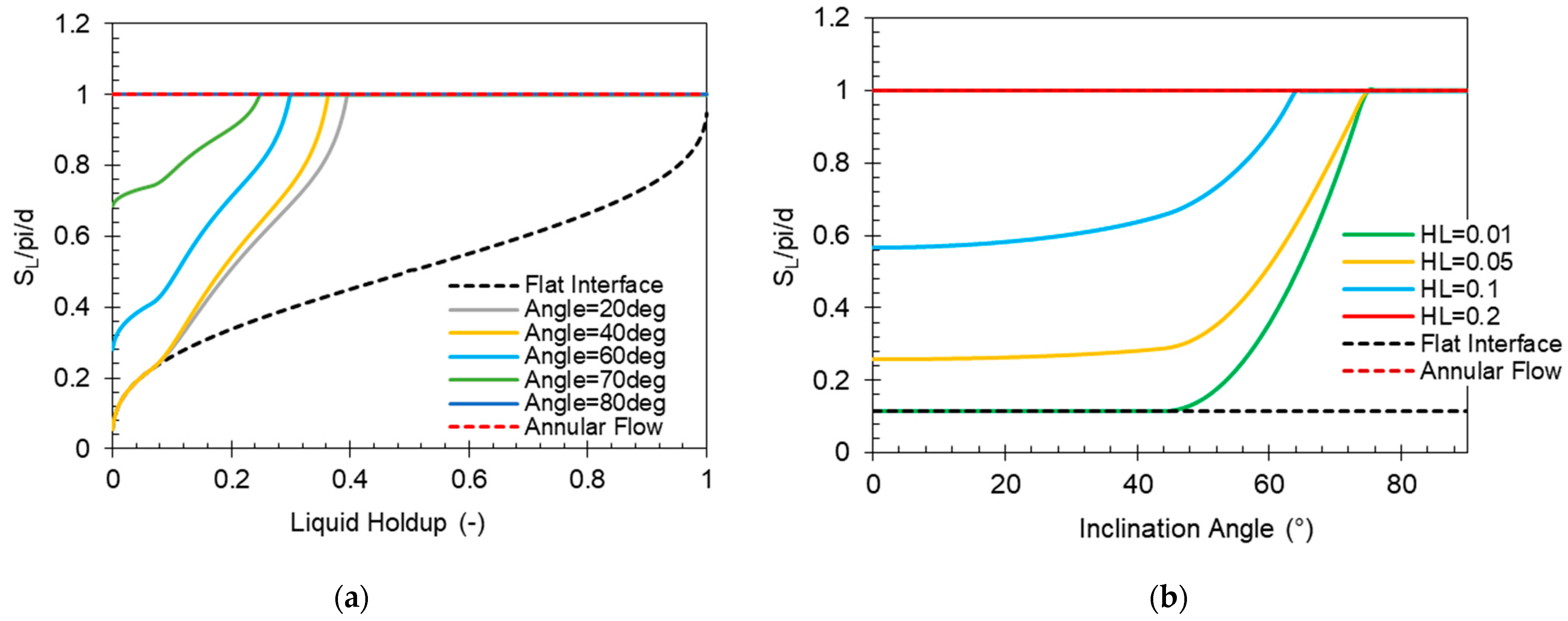
2.1.1. Improved Correlation for Wetted Perimeters

In hopes of developing a generalized method that covers all inclination angles, we propose to use Zhang and Sarica’s (2011) wetted perimeter model [20]. It is currently considered the most comprehensive model available, which captures the effect of H_L, v_SG, and all inclination angles (θ) on the wetted perimeters. However, their model produces less accurate results at low liquid holdup and certain inclination angles. We propose two improvements to correct the model’s performance. At low liquid holdups, the new wetted perimeters are equal to the ones for a flat interface multiplied by an inclination angle correction factor, β. Equations (5)–(10) show the mathematical expressions. H_{L_min} refers to the liquid holdup corresponding to the minimum point on the curve of S_L vs. H_L from the original Zhang and Sarica (2011) [20] wetted perimeter model.

If H_L < H_{L_min},

$$S_{L,C}=S_{L,FI}, S_{C,C}=S_{C,FI}, S_{I,C}=S_{I,FI}, \mathrm{and} h_{ld,C}=h_{ld,FI},$$

(5)

where the subscript C stands for corrected and FI stands for the flat interface.

$$\beta =\left\{\begin{array}{c}0,\hspace{1em}\theta \le 0.25\pi \\ {\left(\frac{\theta -0.25\pi }{0.17\pi }\right)}^2,\hspace{1em}0.25\pi <\theta <0.42\pi \\ 1,\hspace{1em}\theta \ge 0.42\pi \end{array}\right.,$$

(6)

$$S_{L,new}=\pi d\left(\frac{S_{L,C}}{\pi d}+\beta \left(1-\frac{S_{L,C}}{\pi d}\right)\right),$$

(7)

$$S_{C,new}={\pi d-S}_{L,new},$$

(8)

$$S_{I,new}=S_{I,C}+\beta \left(S_{I,AN}-S_{I,C}\right),$$

(9)

$$h_{ld,new}=h_{ld,C}-\beta \left(h_{ld,C}-h_{ld,AN}\right),$$

(10)

where θ is the inclination angle from horizontal in rad; S_L,new is the new liquid wetted perimeter in m; S_C,new is the new gas core wetted perimeter in m; S_L,C is the liquid wetted perimeter with corrections for low H_L in m; S_I,new is the new interfacial perimeter in m; S_I,C is the interfacial perimeter with corrections for low H_L in m; S_I,AN is the interfacial perimeter for annular flow with a uniform distribution assumption in m; h_ld,new is the new dimensionless liquid film thickness at the pipe bottom, -; h_ld,C is the dimensionless liquid film thickness at the pipe bottom with corrections for low H_L, -; h_ld,AN is the dimensionless liquid film thickness for annular flow with a uniform distribution assumption, -.

The dimensionless liquid wetted perimeter, S_L/(πd), from the corrected model is plotted as a function of liquid holdup (H_L) and inclination angle (θ) along with the corresponding values for a flat interface (black dashed line) and annular flow interface (red dashed line) in Figure 2. One can notice that the predicted liquid wetted perimeter gradually changes to annular flow as liquid holdup or inclination angle increases, which is consistent with the experimental observations.

2.1.2. Improved Model for Pressure Gradient Predictions

The total pressure gradient is mainly composed of two components (Equation (11)), i.e., gravitational and frictional pressure gradients. The gravitational pressure drop (Equation (12)) is a function of the liquid holdup, which is calculated from the combined momentum equation with the corrected wetted wall perimeter correlations presented in the previous section. The model’s evaluation shows a fair prediction of liquid holdup, which will be presented in the next section. However, the evaluation shows that the two-fluid model generally overpredicts the pressure gradient even when given the experimental measured liquid holdup. It means that the overprediction is most probably caused by the frictional pressure drop. The frictional pressure drop has two main factors, namely liquid/wall and gas/wall effects. Because the overpredictions were noticed for all conditions including annular flow in vertical pipes, it can be speculated that the issue is with the liquid wall shear stress. This is because the liquid wall interface exists for all cases in segregated flow conditions; on the other hand, the gas wall interface does not exist in annular flow conditions. After establishing that the correction must be done for the liquid wall shear stress, the segregated flow datasets in Table 1 were used to find a correction factor, φ. Correspondingly, the frictional pressure drop can be rewritten in Equation (13). The mathematical expression of φ is given in Equation (14). It is developed based on the observation that the prediction from the original two-fluid model becomes higher as the superficial gas Reynolds number increases for cases with low gas densities, while the factor is almost constant at high gas density (or pressure) conditions.

$$-{\left.\frac{dp}{dL}\right)}_t=-{\left.\frac{dp}{dL}\right)}_g-{\left.\frac{dp}{dL}\right)}_f,$$

(11)

$$-{\left.\frac{dp}{dL}\right)}_g=\left({\rho }_L{H}_L+{\rho }_G\left(1-H_L\right)\right)g\sin \theta ,$$

(12)

$$-{\left.\frac{dp}{dL}\right)}_f=\frac{\phi {\tau }_{WL}{S}_{L,new}}{A_P}+\frac{{\tau }_{WC}{S}_{C,new}}{A_P},$$

(13)

$$\phi =\left\{\begin{array}{c}\hspace{1em}\hspace{1em}\hspace{1em}\hspace{1em}\hspace{1em}\hspace{1em}0.39,\hspace{1em}{\rho }_G>10 \mathrm{kg}/{\mathrm{m}}^3 or {Re}_{SG}\le 200\\ -0.0017\left(\frac{{Re}_{SG}}{1000}-200\right)+0.39,\hspace{1em}{\rho }_G<10 \mathrm{kg}/{\mathrm{m}}^3 and 200<{Re}_{SG}<300 \\ \hspace{1em}\hspace{1em}\hspace{1em}\hspace{1em}\hspace{1em}\hspace{1em} 0.23,\hspace{1em}{\rho }_G<10 \mathrm{kg}/{\mathrm{m}}^3 and {Re}_{SG}\ge 300\end{array}\right.,$$

(14)

$${Re}_{SG}=\frac{{\rho }_G{v}_{SG}d}{{\mu }_G},$$

(15)

where $-{\left.\frac{dp}{dL}\right)}_t$ is the total pressure gradient in Pa/m; $-{\left.\frac{dp}{dL}\right)}_g$ is the gravitational pressure gradient in Pa/m; $-{\left.\frac{dp}{dL}\right)}_f$ is the frictional pressure gradient in Pa/m; ${\tau }_{WL}$ is the liquid wall shear stress determined from Equation (4) in Pa; ${\tau }_{WC}$ is the gas core wall shear stress determined from Equation (4) in Pa; $S_{L,new}$ is the new liquid wetted perimeter in m; $S_{C,new}$ is the new gas core wetted perimeter in m; $A_P$ is the pipe cross-sectional area in m²; ${\rho }_G$ is the gas density in kg/m³; $v_{SG}$ is the superficial gas velocity in m/s; $d$ is the pipe diameter in m; and ${\mu }_G$ is the gas viscosity in Pa‧s.

2.2. Integrated Model Development

This section introduces the integrated model. Our objective is to find a simple integrated multiphase flow model that can be used for downhole pressure predictions for both gas and oil wells with good accuracy. To achieve this goal, the multiphase flow point model incorporated in our integrated modeling consists of three main components: critical gas velocity estimation for the onset of liquid loading and hydraulic multiphase flow models before and after the onset of liquid loading. The proposed model characterizes the flow based on whether liquid loading occurs. Meanwhile, it is significant to find the onset of liquid loading for several reasons. For instance, knowing the location of liquid loading is vital when designing artificial lift processes, such as determining the pump location. In addition, remediation of liquid loading is required to diminish the assurance issues of its tendency to decrease gas production or even kill the well, increase the susceptibility of corrosion, increase the chance of terrain slugging, and trigger system instability. Accurately identifying the location of liquid loading also aids in downhole pressure prediction due to the distinct flow behaviors before and after liquid loading.

The onset of liquid loading corresponds to the transition of the flow pattern from segregated to intermittent flow [21]. This is where the other two components of the model take place. At points where the superficial gas velocity is estimated to be lower than the critical gas velocity and the flow is considered intermittent/bubbly, the drift-flux model is to be used. The drift-flux model works well in flow patterns where liquid volume is high, such as in intermittent and bubbly flow patterns. The drift-flux homogeneous-like approach makes it simple and continuous and, at the same time, captures some physics through slippage. For points where the superficial gas velocity is greater than the critical gas velocity, i.e., segregated (stratified and annular) flow is encountered, the improved two-fluid model previously proposed is to be used.

The marching algorithm, the process illustrated in Figure 3, is used to estimate the pressure profile along the wellbore. The wellbore is divided into N segments. The calculation starts from the wellhead with known wellhead pressure. Iteration is required to estimate the pressure for each segment, as indicated in the flow chart in Figure 3. To determine the pressure at the lower boundary of the (i + 1)^th segment, the first step is to give an initial guess, based on which the average pressure is calculated. Depending on the availability of the fluid composition, we can choose the composition or black oil model to determine the fluid properties (density, viscosity for each phase, and surface tension) and the superficial velocity for each phase. The next step is to determine the critical gas velocity for the (i + 1)^th segments given the flowing conditions and fluid properties. If the superficial gas velocity is greater than the critical gas velocity, the two-fluid model is used to determine the pressure gradient. Otherwise, the drift-flux model is used. A new pressure at the lower boundary of the (i + 1)^th segment is calculated based on the pressure gradient from the previous step. The calculation is repeated until convergence is reached.

Determining the location and the amount of liquid loading is vital in the integrated model, as previously explained. Finding the onset of liquid loading requires estimating the critical gas velocity. To do so, several models exist. The previous models for critical gas velocity prediction can be classified into two categories. The first category is based on liquid droplet removal, and the second is based on liquid film reversal [22]. Some typical models in the first category are by Turner et al. (1969) [23], Coleman et al. (1991) [24], Li et al. (2002) [25], Wang and Liu (2007) [26], and Zhou and Yuan (2010) [26]. These models are simple, but their performances are much less accurate compared to the models based on liquid film reversal, which is believed to be the main cause of liquid loading. Some typical models that are based on liquid film reversal are by Barnea (1986) [27], Luo et al. (2014) [28], Biberg et al. (2015) [29], Shekhar et al. (2017) [30], Fan et al. (2018) [31], and Rastogi and Fan (2020) [22]. However, most models have limited applicability. For instance, the model proposed by Barnea (1986) [27] does not capture the inclination angle effect on the critical gas velocity well. Luo et al. (2014) [28] and Shekhar et al. (2017) [30] capture the effects of inclination angle well but do not capture the liquid flow rate effects well. The model proposed by Rastogi and Fan (2020) [22] is currently considered the most comprehensive model available. In fact, it captures the effects of liquid flow rate, gas density (or pressure), pipe diameter, and inclination angle on the critical gas velocity, significantly outperforming other models. Therefore, we incorporate this model into our integrated model. Details regarding the model’s performance compared to other existing models can be found in Rastogi and Fan (2020) [22]. By incorporating the onset of liquid loading model, the integrated model can determine whether the well is loaded or not, and if yes, it can identify the location where the well starts to be loaded. A case study is presented in Section 3.2 explaining the phenomenon.

After finding the onset of liquid loading and determining that the fluid does not experience segregated flow, the drift-flux model is selected for pressure gradient prediction. Its greatest advantage is its simplicity, differentiability, and relatively high accuracy when applied in fluid flow with high liquid holdup. It satisfies our need for the integrated model to be comprehensive yet continuous. Of the drift-flux models, one of the models with the widest range of applicability to date is the model proposed by Bhagwat and Ghajar (2014) [32]. In their work, they tested their model against 11 others. Their proposed correlation performed consistently better than all the other models in their study. Their model is point-based like most models and is only evaluated using laboratory measurements. Thus, in an effort to test Bhagwat and Ghajar’s (2014) [32] model on field data, the marching algorithm has to be incorporated. In their work, they did not propose a pressure drop calculation method; therefore, Tengensdal et al.’s (1999) [33] method to calculate pressure drop from void fraction was used. This was tested on the five field datasets listed in

Table 2. Field data for integrated model evaluation.

Source		Well Name	Data Points	Properties Range
Field Data	Civitas Resources	-	104	$\theta =-6.5°~90°$; ID $=$ 2″–4″ $Q_{gs}=72~826$; $Q_{os}=108~347$; GOR $= 298~4182$
Literature	Peffer et al. (1988) [36]	-	93	$\theta =90°$; ID $=1.995\mathrm{″}~ 3.958\mathrm{″}$ $Q_{gs}=923~\mathrm{27,400}$; $Q_{os}=8~160$; GOR $= 3.9~1170$;
		Forties	37	$\theta =43.7°~90°$; ID = $3.958″~6.184\mathrm{″}$; $Q_{gs}=738~9184; Q_{os}=2284~\mathrm{27,270}$; GOR $= 0.323~0.337$;
	Asheim (1986) [37]	Ekofisk	50	$\theta =44.8°~90°$; ID = $2.764″~4.892\mathrm{″}$ $Q_{gs}=1671~\mathrm{55,700}$; $Q_{os}=6.7~\mathrm{17,838}$; GOR $= 0.455~3992$
		Prudhoe Bay	29	$\theta =-0.2°$; ID $=$ $11.938″-15.312″$ $Q_{gs}=\mathrm{32,940}~\mathrm{110,015}$; $Q_{os}=\mathrm{44,204}~\mathrm{143,087};$ GOR $= 0.644~0.872$

. The same datasets will be used for the final integrated model evaluation as well. Figure 4 shows the results of the Bhagwat and Ghajar (2014)/Tengensdal et al. (1999) [32,33] model against two other widely used models (Hagedorn and Brown, 1965 [34]; and Beggs and Brill, 1973 [35]) in the industry. It is evident that the Bhagwat and Ghajar (2014)/Tengensdal et al. (1999) [32,33] model using the marching algorithm performs much better in most cases. Hence, in the proposed integrated multiphase flow model, Bhagwat and Ghajar (2014)/Tengensdal et al. (1999) [32,33] will be used for flow patterns that are not segregated.

3. Model Evaluation

This section presents the model evaluation for the improved two-fluid model and the integrated model, respectively.

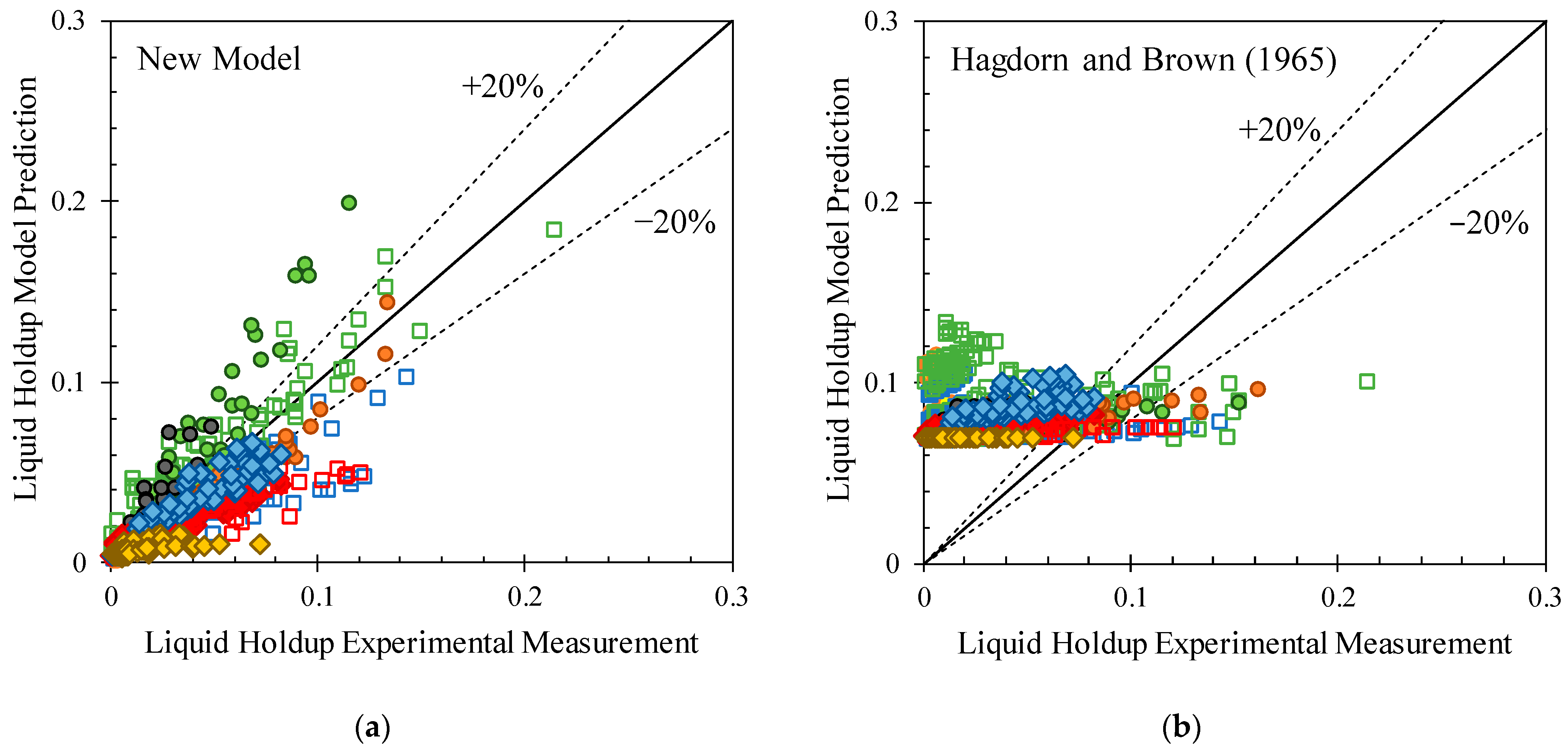
3.1. Two-Fluid Model Evaluation

The two-fluid model’s performance in predicting liquid holdup and pressure gradient was tested against five other existing models using the experimental data listed in Table 1. The models included in the comparison are Hagedorn and Brown (1965) [34], Beggs and Brill (1973) [35], Taitel and Dukler (1976) [5], the Unified model (Zhang et al. 2003 [6]), and Bhagwat and Ghajar (2014) [32]. The comparisons are shown in Figure 5 and Figure 6, followed by tables that summarize the statistical parameters indicating the performance of the models. The average absolute relative errors, ${\mathsf{\epsilon }}_2$, shown in the tables are calculated based on Equation (16). It can be seen from

Table 3. Statistical parameters on liquid holdup prediction.

Dataset\Models	Average Absolute Relative Error
	Zhang et al. (2003) [6]	Bhagwhat and Ghajar (2014) [32]	Beggs and Brill (1973) [35]	Hagedorn and Brown (1965) [34]	Taitel and Dukler (1976) [5]	Improved Model
Magrini (2009) [9]	20.3%	93.4%	30.8%	1635.2%	76.6%	25.6%
Fan (2005) [10]	23.8%	101.6%	44.5%	484.6%	44.2%	24.3%
Meng (1999) [11]	72.6%	63.5%	63.0%	727.9%	221.6%	73.1%
Brill et al. (1995) [12]	40.3%	98.9%	39.2%	149.6%	93.9%	38.8%
Al-Saadi et al. (2015) [3]	34.3%	94.3%	53.5%	244.3%	267.3%	34.4%
Guner et al. (2015) [14]	393.0%	173.1%	39.9%	344.4%	-	44.5%
Fan (2017) [15]	32.2%	66.9%	37.1%	1348.2%	162.7%	33.1%
Rodrigues et al. (2019) [16]	53.1%	42.7%	283.9%	1013.9%	653.4%	53.1%
Alsaadi et al. (2019) [17]	38.3%	96.3%	48.4%	365.8%	285.8%	38.3%
Soedarmo (2019) [18]	32.0%	25.3%	214.5%	769.1%	476.3%	32.0%
Langsholt and Holm (2007) [19]	48.6%	123.7%	198.0%	834.3%	-	48.6%
Total	48.3%	84.7%	86.1%	765.8%	179.7%	37.6%

and

Table 4. Statistical parameters on pressure gradient prediction.

Dataset\Models	Average Absolute Relative Error
	Zhang et al. (2003) [6]	Bhagwhat and Ghajar (2014) [32]	Beggs and Brill (1973) [35]	Hagedorn and Brown (1965) [34]	Taitel and Dukler (1976) [5]	Improved Model
Magrini (2009) [9]	256.6%	252.4%	40.5%	49.7%	43.1%	12.9%
Fan (2005) [10]	56.2%	401.1%	78.9%	105.6%	31.1%	15.4%
Meng (1999) [11]	83.1%	883.3%	67.0%	112.3%	45.3%	33.0%
Brill et al. (1995) [12]	50.2%	1087.3%	21.9%	95.6%	62.4%	64.1%
Al-Saadi et al. (2015) [3]	31.9%	724.6%	10.8%	67.8%	57.5%	41.3%
Guner et al. (2015) [14]	384.0%	635.8%	16.6%	64.3%	-	13.8%
Fan (2017) [15]	14.6%	415.3%	44.0%	47.6%	31.1%	25.6%
Rodrigues et al. (2019) [16]	56.3%	19.5%	10.1%	50.7%	38.1%	12.2%
Alsaadi et al. (2019) [17]	16.7%	1050.4%	51.3%	48.9%	33.5%	28.2%
Soedarmo (2019) [18]	86.0%	26.1%	27.7%	57.2%	30.1%	13.3%
Langsholt and Holm (2007) [19]	9.9%	39.3%	27.1%	33.5%	-	7.1%
Total	83.8%	483.9%	40.3%	69.1%	40.1%	24.0%

that the total average absolute relative errors produced by the improved model are the smallest, indicating that it performed better than the rest of the models.

$${\mathsf{\epsilon }}_2=\frac{1}{N}\sum _{i=1}^N\left|\frac{V_{actual,i}-V_{model,i}}{V_{actual,i}}\right|\times 100\%,$$

(16)

where N is the number of data points; $V_{actual,i}$ is the i^th actual data from experiments or the field; $V_{model,i}$ is the model prediction for the i^th data point.

It is worth mentioning that Andritsos and Hanratty’s (1987) [38] interfacial friction factor correlation was used for liquid holdup predictions in both the current model and the Unified model. By inspection alone, it is clear that the improved model produces more reliable results, especially when predicting the pressure gradient. The liquid holdup predictions, on the other hand, are similar to the predictions produced by the Unified model. This is expected since the only difference from the Unified model in the liquid holdup prediction is the corrected wetted perimeters for low liquid holdup conditions.

The ability of the model to not only predict reliable results but also model the physics is vital. To evaluate the reliability of the model, the results it produces must reflect the physical phenomena. This can be done by comparing the trends produced by the improved model’s results for various properties with their experimental counterparts. Thus, in this section, the parametric analysis was performed on the improved model’s liquid holdup and pressure gradient predictions using the experimental data presented in Table 1. Since most multiphase flow experiments such as the ones in Table 1 were usually controlled by varying v_SG, in this parametric analysis, H_L and dp/dL are plotted vs. v_SG while keeping other parameters constant.

From experimental observation and common sense, as v_SG decreases, liquid holdup increases. In addition, the higher the v_SL the steeper the slope and hence, the larger the rate of change. This was verified by plotting the results from the model with the experimental results in Figure 7. The datasets used to verify this are listed in the legend of the plot. Each color represents a different case of v_SL and dataset combination, and the gas density is marked for each plot. This brings up the next observation. The trend is correctly captured for multiple gas densities, and thus the gas density effect is also captured by the model.

Next, the previous plots were generated for different inclination angles instead of gas density. Again, although the values predicted by the model do not perfectly overlap with the experimental results, the trend is pretty much identical. This suggests that the improved model can capture the inclination angle effects. Figure 8 verifies this observation.

Similar to liquid holdup, the pressure gradient parametric analysis was conducted by comparing the model predictions with experimental data at different flowing conditions. In intermittent flow, the pressure gradient tends to decrease as v_SG increases by decreasing gravitational pressure drop. This is true up to a point where the increase in the frictional pressure drop with v_SG overcomes the decrease in gravitational pressure drop with v_SG. Because the model being evaluated is used when segregated flow is encountered, the flow conditions are beyond the previously explained threshold. Thus, the pressure gradient in the analysis to be shown should always increase with increasing v_SG. This can be verified by the plots in Figure 9 that show the comparison of different gas densities. Figure 10 shows the comparison of various inclination angles instead of gas densities. The overall trend is captured well, although the model’s results are not identical to the experimental readings.

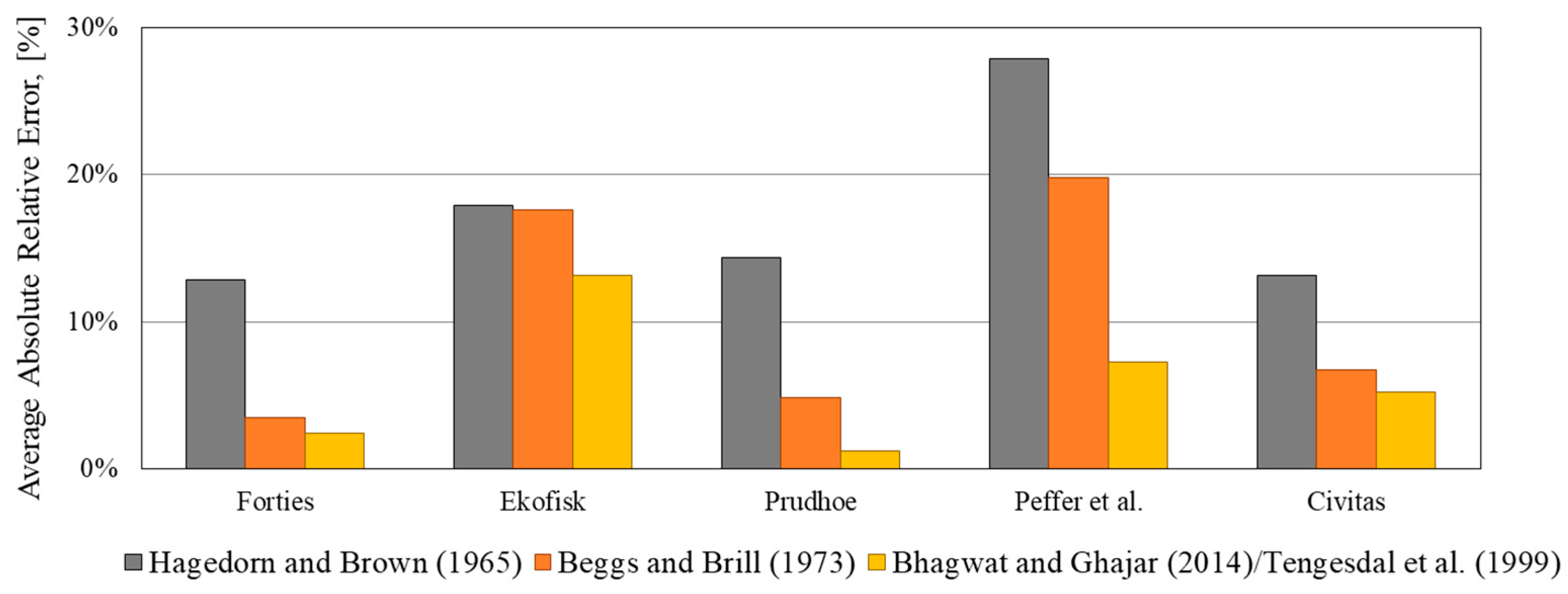
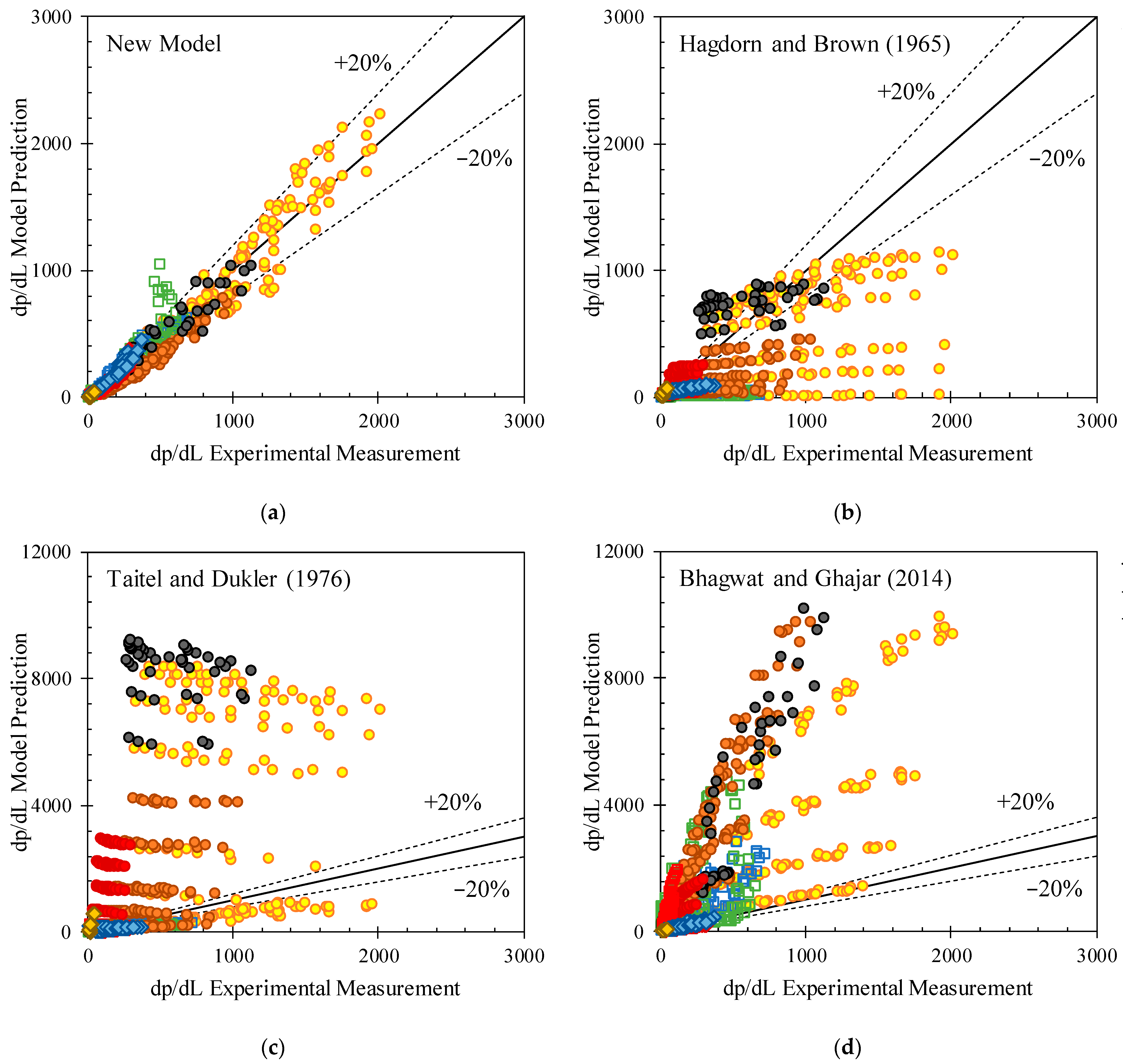
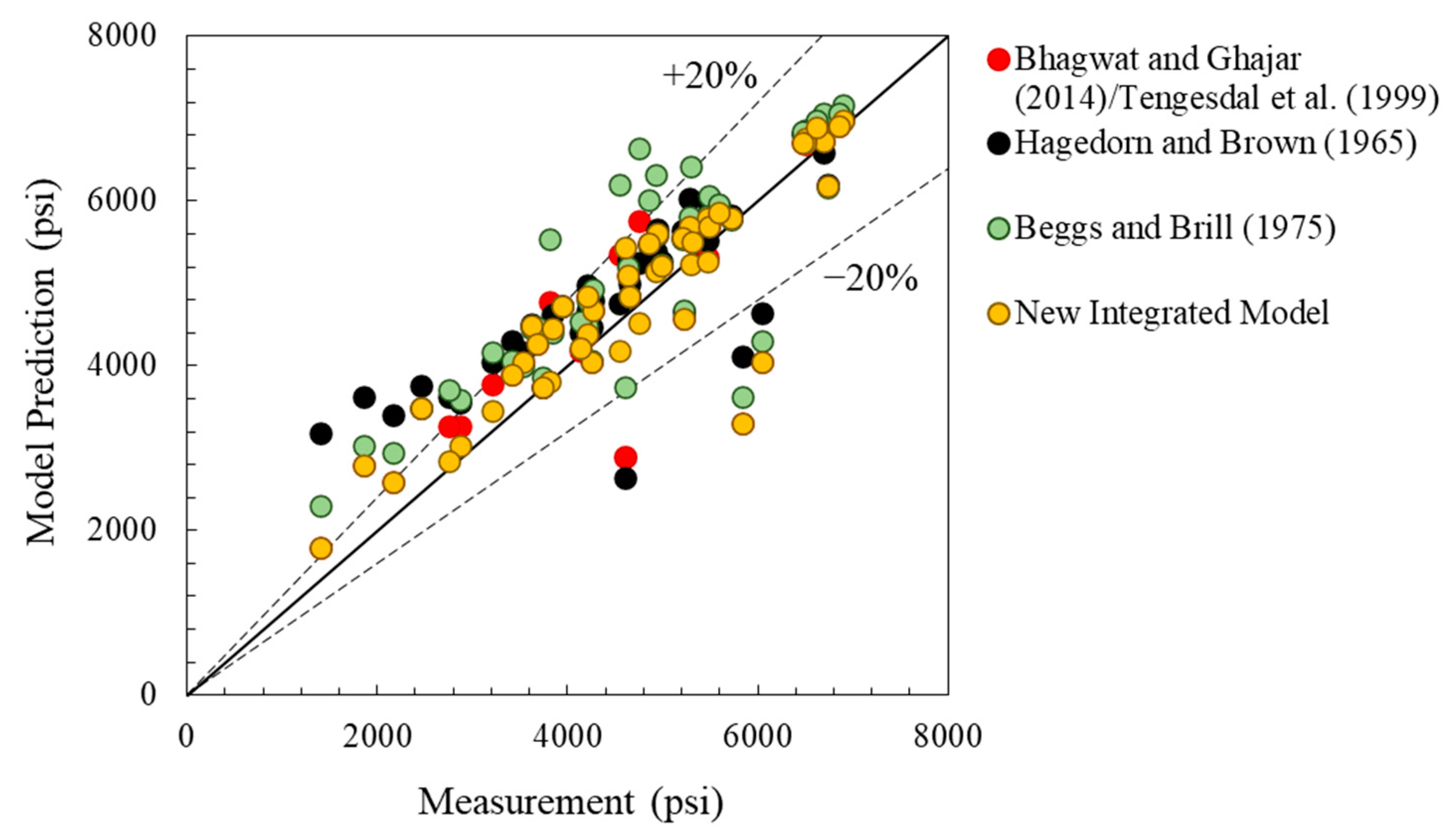
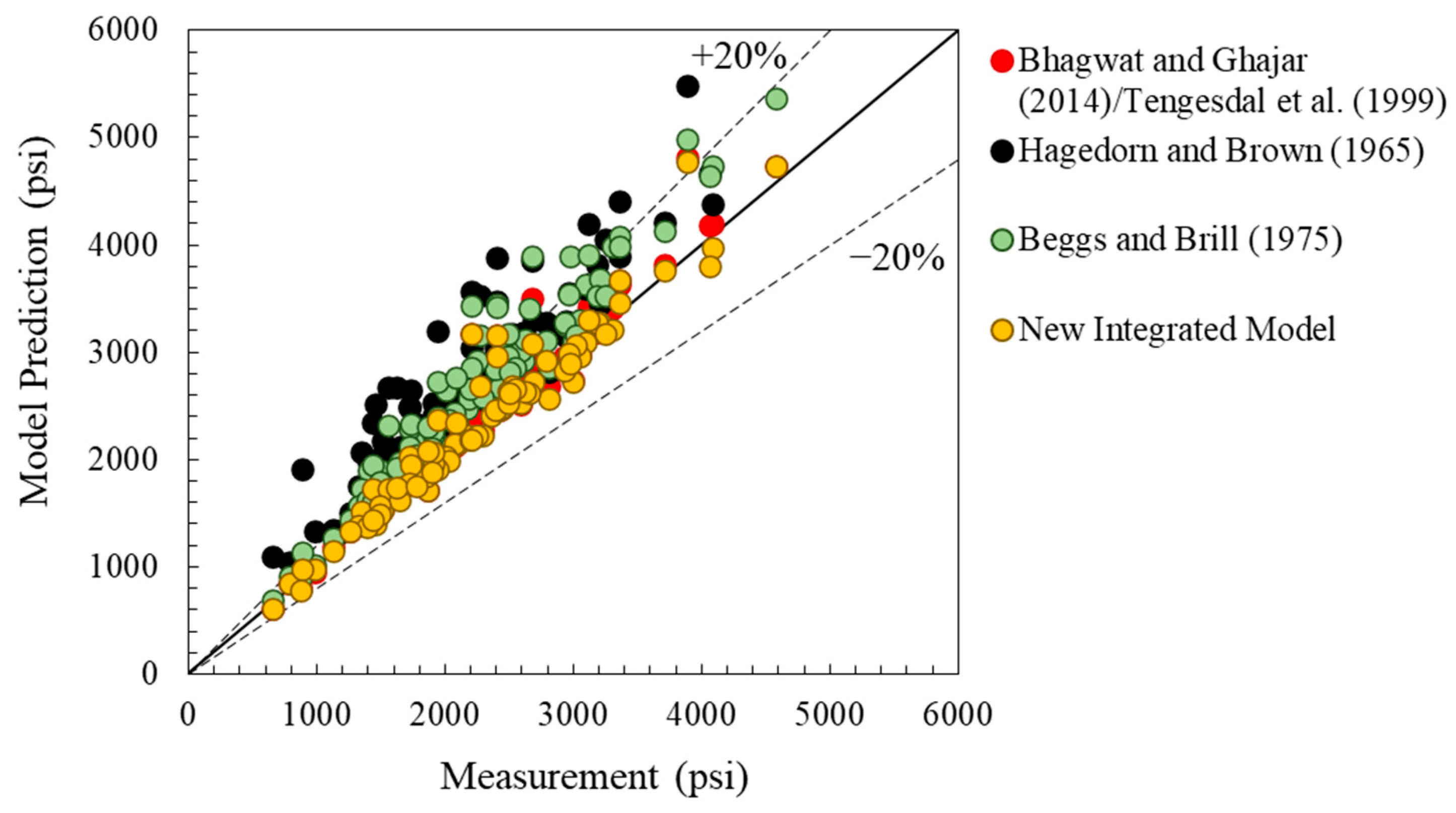
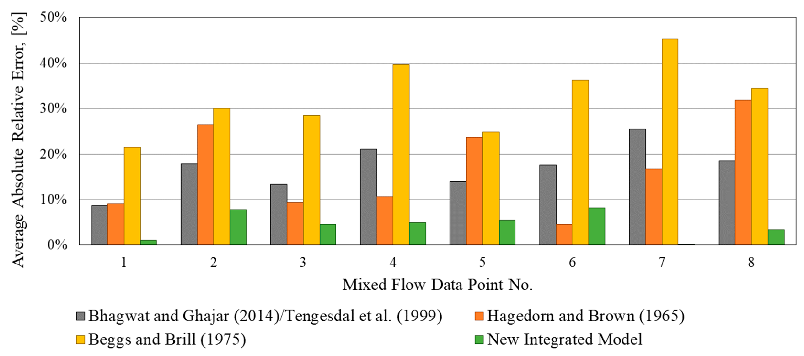
3.2. Integrated Model Evaluation

In this section, the evaluation of the integrated model will be presented, using the field data listed in Table 2. The marching algorithm was used to determine the bottom hole pressure. The procedure has been explained previously and is illustrated in Figure 3. Before presenting the results, a few remarks must be made. Each dataset includes different types of data, and therefore, depending on the availability of the data and the type of reservoir fluid, the procedure may change. In short, the data from Civitas Resources have PVT reports available; thus, the compositional model is used for fluid property determination. Black oil is used for the rest of the dataset. To choose the optimum number of segments for a dataset, a sensitivity analysis on the number of segments was executed. Evidently, as the number of segments increases, the accuracy increases, and consequently, the runtime increases. Thus, in hopes of finding the intrinsic cutoff between accuracy and runtime, the sensitivity analysis was performed on the number of segments of up to 100. Results show that above roughly 30 segments, the increase in accuracy becomes insignificant (<1%). Therefore, in this work, the results are shown for wells segmented into 30 segments. Of the datasets presented in Table 2, only the datasets on the wells from Peffer et al. (1988) [36] and Ekofisk wells from Asheim (1986) [37] experienced both segregated and intermittent flow conditions. The others, on the other hand, only experienced intermittent or bubbly flow conditions. Therefore, for those datasets, the new integrated model will give the same results as the ones produced by Bhagwat and Ghajar (2014)/Tengensdal et al. (1999) [32,33]. For this reason, only the parity plots produced by testing the model using Peffer et al. (1988) [36] and Ekofisk wells from Asheim (1986) [37] will be shown in this evaluation. The corresponding parity plots are shown in Figure 11 and Figure 12, respectively.

Overall, the parity plots show that both Bhagwat and Ghajar (2014)/Tengensdal et al. (1999) [32,33] and the new integrated model perform well, with the new integrated model being slightly better. The similarity found in the results is due to the fact that many of the data points experience intermittent/bubbly flow. Thus, the slight improvement of the new integrated model is owed to the data points that experience segregated flow or both segregated and intermittent flows together. Furthermore, to assess the model better, the data points in which the segregated and intermittent flows exist in the same well were evaluated and are presented below. This shows how the new integrated model performs when dealing with both ends of the spectrum. Evidently, the new integrated model performed exceptionally well for the cases in which both segregated and intermittent flow conditions existed. Figure 13 shows the percent error of each model in predicting the bottom-hole pressure for the data points with mixed flow patterns.

To better illustrate how the model deals with mixed flow conditions, Figure 14, Figure 15 and Figure 16 are presented. Shown in the figures are three cases selected from the Ekofisk dataset. Figure 14 shows the case where the flow is segregated across the entirety of the well. This can be noticed from the curves of v_SG and v_SGc. The v_SG curve (black) has not yet crossed the v_SGc curve (red), and thus, liquid loading has not occurred. The liquid holdup is relatively low in this case. However, it is noticed that they are approaching each other. In this case, the new integrated model would use the improved two-fluid model to calculate liquid holdup and pressure gradient for the entirety of the well. Figure 15, on the other hand, shows the case where the flow is intermittent or bubbly across the entirety of the well. This can be noticed from the curves of v_SG and v_SGc. The v_SG curve (black) has already crossed the v_SGc curve (red), and thus, liquid loading has occurred, hence the relatively high liquid holdup. In this case, the new integrated model would use Bhagwat and Ghajar (2014)/Tengensdal et al. (1999) [32,33] to calculate liquid holdup and pressure gradient for the entirety of the well. Finally, Figure 16 shows the case in which both flow patterns occur (mixed flow case). In this case, liquid loading occurs in the well during the flow. The onset of liquid loading in this case occurs at around 2000 m of measured depth. This is where the two curves cross. For this case, the new integrated model would use the improved two-fluid model for segments of the well that are above the location of the onset of liquid loading (~2000 m) and Bhagwat and Ghajar (2014)/Tengensdal et al. (1999) [32,33] for the ones below it. This is reflected in the deviation of the pressure and liquid holdup curves at the onset of liquid loading (~2000 m).

To conclude the evaluation of the new integrated model, a summary of all the results is presented in the bar graph in Figure 17. The column before the last, titled “Mixed Flow Pattern”, shows the average absolute relative percent error of the models’ predictions of bottom-hole pressure for the data points that experience liquid loading along the flow (i.e., both segregated and intermittent flow occurs in the well). The total average absolute percent error for each model for all the datasets is shown in the last column. All in all, the new integrated model provided the lowest average percent absolute relative error (5.1%) in predicting bottom-hole pressures for all the datasets.

4. Discussion

The model evaluation shows that the new two-fluid model improves the pressure gradient prediction dramatically when compared with other existing models (Figure 6 and Table 4). As a result, it improves the bottom-hole pressure predictions for wells that experience segregated flow, as demonstrated in Figure 11, Figure 12 and Figure 13. Drawing from these observations, the proposed integrated model is expected to be effective for both oil and gas wells across diverse flowing conditions.

Most of the existing state-of-the-art two-fluid models for segregated flow require the user to select the interfacial friction factor (f_I) correlation, such as the Unified model [6]. This provides flexibility but, in the meantime, increases the complexity because of the f_I correlation selection and the fact that dozens of interfacial friction factor correlations are available in the literature. Each was developed for different flowing conditions or using different databases [8]. Hence, one of the advantages of the proposed integrated model is that it eliminates the need for changing f_I correlations when the flowing condition varies, which reduces the complexities associated with closure relationship selection and alteration.

However, we think there is still room for model improvement. First, the literature has limited medium/high-viscosity experimental data on segregated gas–liquid flow. Having more of such data would aid in the two-fluid model’s improvement in terms of the viscosity effect on fluid flow behaviors. Further experimental and theoretical studies are required to address this issue. Furthermore, although the drift-flux model by Bhagwat and Ghajar (2014) [32] gives reasonable predictions for most of the field cases that experience intermittent/bubbly flow conditions in this study, detailed parametric studies are required to evaluate its performance using laboratory experimental data or more field data. This will be the target of our future work.

The significance of predicting the bottom-hole pressure and the wellbore pressure profile has been introduced previously. To effectively assess the model’s performance in these predictions, more field data are required. It is unfortunate that field data are quite scarce in the open literature. However, as more field data become accessible, the associated modeling studies will be significantly enhanced.

5. Conclusions

This work presents an integrated model for downhole pressure predictions. It also improves the classic two-fluid model for pressure gradient and liquid holdup predictions in segregated flow. The new integrated model classifies the flow based on the onset of liquid loading. The model uses the drift-flux model if liquid loading occurs and the improved two-fluid model if it does not. The proposed two-fluid model outperformed five other models in predicting the liquid holdup and pressure gradient of 11 experimental datasets. In addition, the model succeeds in capturing the effects of inclination angle, gas density, and liquid and gas superficial velocities on liquid holdup and pressure gradient. The new model eliminates the need for changing interfacial friction factor correlations when the flowing condition varies, which can reduce the complexities associated with closure relationship selection and alteration. Moreover, the new integrated model outperformed the other multiphase flow models in predicting the downhole pressure of 313 field data points. When dealing with wells that have both segregated and intermittent flow, the new model produces outstanding results. In addition, it succeeds in finding the location and amount of liquid loading in a well, paving the way for the design and optimization of artificial lift processes that require such knowledge.

References

1. Beggs, H.D. Production Optimization Using NODAL Analysis; Society of Petroleum Engineers: Richardson, TX, USA, 2003. [Google Scholar]
2. Ishinbaev, N.A.; Krasnov, A.N.; Yu Prakhova, M.; Novikova, Y.V. Analysis of the Downhole Measurement System’s Pressure and Temperature Measuring Channel Calibration Errors. J. Phys. Conf. Ser. 2021, 2096, 012066. [Google Scholar] [CrossRef]
3. Shoham, O. Mechanistic Modeling of Gas-Liquid Two-Phase Flow in Pipes; Society of Petroleum Engineers: Richardson, TX, USA, 2006. [Google Scholar]
4. PIPESIM 2019—Steady-State Multiphase Flow Simulator. Available online: https://www.software.slb.com/-/media/software-media-items/software/documents/external/product-sheets/20-is-000057_pipesim_2019_technical_description.pdf (accessed on 1 November 2023).
5. Taitel, Y.; Dukler, A.E. A model for predicting flow regime transitions in horizontal and near horizontal gas-liquid flow. AIChE J. 1976, 22, 47–55. [Google Scholar] [CrossRef]
6. Zhang, H.-Q.; Wang, Q.; Sarica, C.; Brill, J.P. Unified Model for Gas-Liquid Pipe Flow via Slug Dynamics—Part 1: Model Development. J. Energy Res. Technol. 2003, 125, 266–273. [Google Scholar] [CrossRef]
7. Xiao, J.J.; Shonham, O.; Brill, J.P. A Comprehensive Mechanistic Model for Two-Phase Flow in Pipelines. In Proceedings of the SPE Annual Technical Conference and Exhibition, New Orleans, LA, USA, 23–26 September 1990. SPE-20631-MS. [Google Scholar]
8. Rastogi, A.; Fan, Y. Machine learning augmented two-fluid model for segregated flow. Fluids 2022, 7, 12. [Google Scholar] [CrossRef]
9. Magrini, K.L. Liquid Entrainment in Annular Gas-liquid Flow in Inclined Pipes. Master’s Thesis, The University of Tulsa, Tulsa, OK, USA, 2009. [Google Scholar]
10. Fan, Y. An Investigation of Low Liquid Loading Gas-Liquid Stratified Flow in Near-horizontal Pipes. Ph.D. Thesis, The University of Tulsa, Tulsa, OK, USA, 2005. [Google Scholar]
11. Meng, W. Low Liquid Loading Gas-Liquid Two-Phase Flow in Near-Horizontal Pipes. Ph.D. Thesis, The University of Tulsa, Tulsa, OK, USA, 1999. [Google Scholar]
12. Brill, J.P.; Chen, X.T.; Flores, J.G.; Marcano, R. Transportation of Liquids in Multiphase Pipelines under Low Liquid Loading Conditions; Final Report; The Pennsylvania State University: Pennsylvania, PA, USA, 1995. [Google Scholar]
13. Alsaadi, Y.; Pereyra, E.; Torres, C.; Sarica, C. Liquid Loading of Highly Deviated Gas Wells from 60° to 88°. In Proceedings of the SPE Annual Technical Conference and Exhibition, Houston, TX, USA, 28–30 September 2015. [Google Scholar]
14. Guner, M.; Pereyra, E.; Sarica, C.; Torres, C. An Experimental Study of Low Liquid Loading in Inclined Pipes from 90° to 45°. In Proceedings of the SPE Production and Operations Symposium, Oklahoma City, OK, USA, 1–5 March 2015. [Google Scholar] [CrossRef]
15. Fan, Y. A Study of the Onset of Liquid Accumulation and Pseudo-slug Flow Characterization. Ph.D. Thesis, University of Tulsa, Tulsa, OK, USA, 2017. [Google Scholar]
16. Rodrigues, H.T.; Pereyra, E.; Sarica, C. Pressure effects on low-liquid-loading oil/gas flow in slightly upward inclined pipes: Flow pattern, pressure gradient, and liquid holdup. SPE J. 2019, 24, 2221–2238. [Google Scholar] [CrossRef]
17. Alsaadi, Y. Low Liquid Loading Two-Phase and Three-Phase Flows in Slightly Upward Inclined Pipes. Ph.D. Thesis, University of Tulsa, Tulsa, OK, USA, 2019. [Google Scholar]
18. Soedarmo, A.A. Gas-Oil Flow in Upward-Inclined Pipes: Pseudo-Slug Flow Modeling and Upscaling Studies. Ph.D. Thesis, The University of Tulsa, Tulsa, OK, USA, 2019. [Google Scholar]
19. Langsholt, M.; Holm, H. Liquid Accumulation in Gas-Condensate Pipelines—An Experimental Study. In Proceedings of the 13th International Conference on Multiphase Production Technology, Edinburgh, UK, 13–15 June 2007. [Google Scholar]
20. Zhang, H.-Q.; Sarica, C. A model for wetted-wall fraction and gravity center of liquid film in gas/liquid pipe flow. SPE J. 2011, 16, 692–697. [Google Scholar] [CrossRef]
21. Fan, Y.; Pereyra, E.; Sarica, C.; Schleicher, E.; Hampel, U. Analysis of flow pattern transition from segregated to slug flow in upward inclined pipes. Int. J. Multiph. Flow 2019, 115, 19–39. [Google Scholar] [CrossRef]
22. Rastogi, A.; Fan, Y. Experimental and modeling study of onset of liquid accumulation. J. Nat. Gas. Sci. Eng. 2020, 73, 103064. [Google Scholar] [CrossRef]
23. Turner, R.G.; Hubbard, M.G.; Dukler, A.E. Analysis and prediction of minimum flow rate for the continuous removal of liquids from gas wells. J. Pet. Technol. 1969, 21, 1475–1482. [Google Scholar] [CrossRef]
24. Coleman, S.B.; Clay, H.B.; McCurdy, D.G.; Norris, L.H. A new look at predicting gas-well load-up. J. Pet. Technol. 1991, 43, 329–333. [Google Scholar] [CrossRef]
25. Li, M.; Lei, S.; Li, S. New View on Continuous-Removal Liquids from Gas Wells. SPE Prod. Fac. 2002, 17, 42–46. [Google Scholar] [CrossRef]
26. Wang, Y.Z.; Liu, Q.W. A New Method to Calculate the Minimum Critical Liquid Carrying Flow Rate for Gas Wells. Pet. Geol. Oilfield Dev. Daqing 2007, 6, 82–85. [Google Scholar]
27. Barnea, D. Transition from annular flow and from dispersed bubble flow—Unified models for the whole range of pipe inclinations. Int. J. Multiph. Flow 1986, 12, 733–744. [Google Scholar] [CrossRef]
28. Luo, S.; Kelkar, M.; Pereyra, E.; Sarica, C. A new comprehensive model for predicting liquid loading in gas wells. SPE Prod. Oper. 2014, 29, 337–349. [Google Scholar] [CrossRef]
29. Biberg, D.; Hoyer, N.; Holm, H. Accounting for flow model uncertainties in gas-condensate field design using the OLGA High Definition Stratified Flow Model. In Proceedings of the 17th International Conference on Multiphase Production Technology, Cannes, France, 10–12 June 2015. BHR-2015-G5. [Google Scholar]
30. Shekhar, S.; Kelkar, M.; Hearn, W.J.; Hain, L.L. Improved prediction of liquid loading in gas wells. SPE Prod. Oper. 2017, 32, 539–550. [Google Scholar] [CrossRef]
31. Fan, Y.; Pereyra, E.; Sarica, C. Onset of liquid-film reversal in upward-inclined pipes. SPE J. 2018, 23, 1630–1647. [Google Scholar] [CrossRef]
32. Bhagwat, S.M.; Ghajar, A.J. A flow pattern independent drift flux model based void fraction correlation for a wide range of gas–liquid two phase flow. Int. J. Multiph. Flow 2014, 59, 186–205. [Google Scholar] [CrossRef]
33. Tengesdal, J.Ø.; Kaya, A.S.; Sarica, C. Flow-pattern transition and hydrodynamic modeling of churn flow. SPE J. 1999, 4, 342–348. [Google Scholar] [CrossRef]
34. Hagedorn, A.R.; Brown, K.E. Experimental study of pressure gradients occurring during continuous two-phase flow in small-diameter vertical conduits. J. Pet. Technol. 1965, 17, 475–484. [Google Scholar] [CrossRef]
35. Beggs, D.H.; Brill, J.P. A study of two-phase flow in inclined pipes. J. Pet. Technol. 1973, 25, 607–617. [Google Scholar] [CrossRef]
36. Peffer, J.W.; Miller, M.A.; Hill, A.D. An improved method for calculating bottomhole pressures in flowing gas wells with liquid present. SPE Prod. Eng. 1988, 3, 643–655. [Google Scholar] [CrossRef]
37. Asheim, H. MONA, an accurate two-phase well flow model based on phase slippage. SPE Prod. Eng. 1986, 1, 221–230. [Google Scholar] [CrossRef]
38. Andritsos, N.; Hanratty, T.J. Interfacial instabilities for horizontal gas-liquid flows in pipelines. Int. J. Multiph. Flow 1987, 13, 583–603. [Google Scholar] [CrossRef]
Figure 1. Forces and parameters in segregated flow two-fluid model.
Energies 16 07923 g001
Figure 2. Dimensionless wetted liquid perimeter (SL/pi/d) as a function of liquid holdup (a) and inclination angle (b) from the new model.
Energies 16 07923 g002
Figure 3. Integrated model flow chart.
Energies 16 07923 g003
Figure 4. Average absolute relative error of model performance on bottom-hole pressure predictions for various datasets [32,33,34,35,36].
Energies 16 07923 g004
Figure 5. Liquid holdup comparison between experimental measurement and model predictions. Predictions produced by each model are plotted against the experimental values. Different colors and shapes are used to distinguish between datasets. Points on the solid line indicates that the predicted values equal their experimental counterpart. Points on the +20% and 20% dashed lines indicate that the predicted values are +20% or 20% than their experimental counterpart. In other words, the further the points are from the solid line the larger the difference between the predicted and the actual value [5,6,32,34,35].
Energies 16 07923 g005aEnergies 16 07923 g005b
Figure 6. Pressure gradient (dp/dL) comparison between experimental measurement and model predictions. Predictions produced by each model are plotted against the experimental values. Different colors and shapes are used to distinguish between datasets. Points on the solid line indicates that the predicted values equal their experimental counterpart. Points on the +20% and 20% dashed lines indicate that the predicted values are +20% or 20% than their experimental counterpart. In other words, the further the points are from the solid line the larger the difference between the predicted and the actual value [5,6,32,34,35].
Energies 16 07923 g006aEnergies 16 07923 g006b
Figure 7. Liquid holdup (HL) vs. gas flow rate of experimental data against model prediction for different gas densities [16,18].
Energies 16 07923 g007
Figure 8. Liquid holdup (HL) vs. superficial gas velocity (vSG) of experimental data against model prediction for different inclination angles [9,13,14,15].
Energies 16 07923 g008
Figure 9. Pressure gradient (dp/dL) vs. gas flow rate of experimental data against model prediction for different gas densities [16,18].
Energies 16 07923 g009
Figure 10. Pressure gradient (dp/dL) vs. superficial gas velocity (vSG) of experimental data against model prediction for different inclination angles (θ) [9,13,14,15].
Energies 16 07923 g010
Figure 11. Bottom-hole pressure model prediction against measurement for Ekofisk wells from Asheim (1986) [37]. Refs. [32,33,34,35].
Energies 16 07923 g011
Figure 12. Bottom-hole pressure model prediction against measurement for Peffer et al. (1988) [36] dataset [32,33,34,35].
Energies 16 07923 g012
Figure 13. Average absolute relative error of models’ performances in predicting the bottom-hole flowing pressure of mixed flow pattern points [32,33,34,35,37].
Energies 16 07923 g013
Figure 14. Critical gas velocity (vSGc), superficial gas velocity (vSG), pressure, and liquid holdup as a function of measured depth for segregated flow case.
Energies 16 07923 g014
Figure 15. Critical gas velocity (vSGc), superficial gas velocity (vSG), pressure, and liquid holdup as a function of measured depth for intermittent/bubbly flow case.
Energies 16 07923 g015
Figure 16. Critical gas velocity (vSGc), superficial gas velocity (vSG), pressure, and liquid holdup as a function of measured depth for mixed flow case.
Energies 16 07923 g016
Figure 17. Statistics of the new integrated model evaluation [32,33,34,35,36,37].
Energies 16 07923 g017