Abstract
In this work, a model to estimate circumsolar normal irradiance (CSNI) for several half-opening angles under clear skies was developed. This approach used a look-up table to determine the model parameters and estimate CSNI for half-opening angles between 0.5° and 5°. To develop and validate the proposed model, data from five locations worldwide were used. It was found that the proposed model performs better at the locations under study than the models available in the literature, with relative mean bias error ranging from −13.94% to 0.70%. The impact of CSNI for these different half-opening angles on concentrating solar power (CSP) systems was also studied. It was found that neglecting CSNI could lead to up to a 7% difference between the direct normal irradiance (DNI) measured by a field pyrheliometer and the DNI that is captured by CSP systems. Additionally, a case study for parabolic trough concentrators was performed as a way to estimate the impact of higher circumsolar ratios (CSR) on the decrease of the intercept factor for these systems. It was also concluded that if parabolic trough designers aim to reduce the impact of CSNI variation on the intercept factor, then parabolic troughs with higher rim angles are preferred.
1. Introduction
Concentrating solar power (CSP) systems highly depend on the intensity of direct normal irradiance (DNI) in their aperture angle [1]. Therefore, it is crucial that designers have access to accurate DNI data to avoid compromising the proper operation and economic viability of such systems. The most reliable way of obtaining accurate DNI data is to use a ground-based station equipped with a pyrheliometer in a sun-tracker system. This instrument needs to track the apparent movement of the sun along its path in the sky to measure the direct beam. However, as this tracking cannot be done with perfect accuracy, these instruments are designed in such a way that they receive radiation not only from the solar disk but also from the surrounding area, known as the circumsolar region [2]; that is, the aperture half-angle of the instrument is larger than the apparent sun disk radius in order to accommodate the tracking misalignments and errors. On the other hand, this radiosity in the circumsolar region around the sun disk, known as circumsolar irradiance, is not negligible when designing CSP systems, because these systems usually have opening half-angles lower than those of the pyrheliometers, depending on the concentration factor.
The World Meteorological Organization (WMO) recommends that pyrheliometers have an opening half-angle of 2.5° to enable a fair comparison between the DNI measured at different locations around the globe [3]. However, the upper limit of the opening half-angles of common CSP technologies such as parabolic trough, linear Fresnel, dish-Stirling and solar tower are 0.8°, 1.0°, 1.6°, and 1.8°, respectively [2,4], that is, lower than the standard aperture half-angles of pyrheliometers. In other words, CSP systems will not receive the same levels of irradiance as measured by collocated standard pyrheliometers. This difference will increase when the circumsolar radiosity also increases as a result of solar radiation scattering in the atmosphere due to a higher concentration of aerosols. The quantification of this difference between the measured DNI and the DNI that is reflected by the mirrors of a given CSP system is one of the main motivations of this study.
The air molecules, aerosols, and cirrus clouds scatter the sun rays from the sun disk region to the circumsolar region [5]. When this irradiance is measured in a surface normal to the sun line, it is known as circumsolar normal irradiance (CSNI). In that sense, while experimental values of DNI obtained from pyrheliometer measurements are related only to the total scattering effect and transmittance of the atmosphere, the CSNI is also related to the angular distance from the center of the sun disk, i.e., the scattering angle [6,7]. On the other hand, measurement of CSNI is not straightforward because of the sharp decrease in intensity between the edge of the sun disk and the limit of the field of view of the instrument [2]. However, some attempts to measure CSNI have been made and a review on these can be found in Abreu et al. [6].
Regarding CSNI modelling, it is usually carried out using radiative transfer models (RTM) such as libRadtran [8]. However, because RTM models often need high-quality atmospheric data such as aerosol optical depth and precipitable water vapor, some authors have proposed simpler models to predict CSNI. In these models, CSNI is usually estimated as a function of more commonly available solar irradiance data and presented as a circumsolar ratio (CSR), i.e., the ratio between CSNI and DNI [5,6,9,10]. Such models are defined for a fixed aperture angle except the model from Eissa et al. [5] in which, in addition, the authors presented a way of varying the aperture angle. This takes a similar form of the fixed aperture angle model, but the model coefficients are determined using a sixth-degree polynomial of the aperture angle and allows the CSNI to be estimated for any defined aperture angle in the range of 0.4°–5.0°. Although the model of Abreu et al. [6] was initially developed for a fixed aperture angle, the way it was constructed also allows its generalization for any aperture angle, with the advantage that it only needs widely available solar irradiance data to predict CSNI; this being one of the main objectives of this study.
Furthermore, information on CSNI is crucial for the design and operation of CSP systems. In CSP plants, the solar irradiance is focused onto an absorber using mirrors [11]. However, due to the difference between the opening half-angles of the pyrheliometers and the CSP systems mentioned above, the use of less accurate DNI data (without correctly accounting for the differences of the opening half-angle, that is, without considering CSNI) leads to incorrect assumptions about the solar irradiance that is focused by the CSP mirrors onto the receiver. This will increase the uncertainty of the energy generation predictions of CSP systems, which ultimately increases the difficulty of its operation.
The impact of CSNI on CSP systems can be assessed using a variety of tools, namely, ray tracing tools, analytical optical performance models, and models that use look-up tables or parametrizations of the solar position relative to the CSP mirrors [2]. Ray tracing models describe the solar irradiance as a multitude of solar rays that originate from the sun, reach the concentrator, and finally the receiver. Examples of ray tracing models can be STRAL [12] and MIRVAL [13], to name a few. Analytical models use logical equations that can describe the ray’s path through the optical system. Examples of analytical models are the Bendt-Rabl model [14] and the HFLCAL method [15], to name a few. Lastly, models based on look-up tables use parametrizations or look-up tables to assess the optical performance of a CSP collector according to the solar position. SAM [16] and Greenius [17,18] are examples of models that use a look-up table. The approach followed in this study was to use an analytical model to determine how the intercept factor (the ratio of the irradiance reaching the receiver over the incident irradiance) is affected according to CSR.
In this work, a simple and fast model to derive CSNI is proposed for clear-sky conditions at any desired aperture angle. In other words, the proposed model is able to determine the CSNI that reaches the receiver of any CSP system, such as parabolic troughs, tower systems, or dish systems, to name a few. The developed model also aims to identify the difference between using ground-based DNI measurements (for the aperture half-angle of the field pyrheliometer) and DNI modelled data according to the aperture half-angles of typical CSP technologies (with lower aperture angles) at several locations around the globe. This allows quantification of the errors associated with using directly measured DNI data on the simulation of CSP systems. To the authors’ best knowledge, the model proposed in this work is the only fast and simple model capable of estimating CSNI at several locations in more than one climate zone, which constitutes another novelty here. Furthermore, the impact of CSNI on CSP systems, specifically in parabolic trough systems, was also studied using the analytical optical performance model from Bendt and Rabl [14].
2. Data
2.1. Experimental Solar Radiation Data
In this work, CSNI data corresponding to several half-opening angles necessary to develop the proposed model were obtained using the version 1.7 of the libRadtran RTM [8] simulations based on AERONET [19] input data for five locations worldwide. AERONET is a ground-based aerosol network that has provided aerosol optical data and microphysical and radiative properties for aerosol research and characterization for more than 25 years. The values retrieved from the AERONET database were the following: aerosol optical depth, aerosol single scattering albedo, aerosol phase function, surface albedo, and precipitable water vapor. The AERONET data were retrieved at the wavelengths of 440 nm, 675 nm, 870 nm, and 1020 nm. However, the simulations were carried out for the wavelength interval between 200 nm and 5000 nm. This wavelength interval covers not only the spectral response of a conventional pyrheliometer (300–4000 nm) but also the spectral response of windowless absolute cavity radiometers (the 5000 nm upper limit), against which field pyrheliometers are commonly calibrated. To extrapolate the AERONET aerosol data to 200 nm and 5000 nm, Ångström’s law was used. For further details on this process, the reader can consult a previous work by Abreu et al. [6]. Ground-based DNI values from the BSRN database were also used in the validation process of the CSNI data for the same locations. BSRN is a network of ground-based radiometric stations with the aim of detecting changes in the solar radiation field at the Earth’s surface [20].
The five locations analyzed in this work are scattered around the globe and have collocated AERONET and BSRN stations, thus allowing measurements to be assumed from both stations at close timestamps. The time difference between AERONET and the radiometric stations data is not higher than 1 min and therefore it is assumed that, under clear skies, they are representative of the same atmospheric conditions. More information about the locations is presented in Table 1.

Table 1.
Information on the AERONET and radiometric stations and data period used in this work. Legend: Lat.—Latitude, Long.—Longitude, Alt.—Altitude, TR—Tropical, TM—Temperate, AR—Arid.
Regarding data quality control, AERONET data Level 1.5 Version 3 was used here for the following two main reasons: to use single scattering albedo measurements instead of mean values, and because the Version 3 processing algorithm marks a significant improvement in the quality control of the sun photometer AOD measurements, eliminating the need for manual quality control and cloud screening by an analyst [21,22]. Concerning solar radiation data, the quality filters from BSRN [20] were used to ensure that extremely rare or physically impossible values were discarded.
The quality control procedure used here ensures the following: (i) that the simulations to determine DNI and CSNI are as accurate as possible; (ii) that the model developed here was created and validated using the most accurate solar irradiance ground-based data available. Moreover, the data used in this work were screened and classified as clear sky by the AERONET algorithm alongside solar radiation data from collocated radiometric stations, in order to ensure that both AERONET and BSRN/Evora data are representative of the same atmospheric conditions.
2.2. Modelled DNI and CSNI Data
In this work, modelled DNI and CSNI data from the libRadtran RTM are used to develop the proposed CSNI model. The generation of these kind of data is complex because of (i) the availability and processing of the required inputs, (ii) the computation time required to simulate extensive datasets such as the one used here. Therefore, the DNI and CSNI data were generated and validated in a previous work from the same authors [6]. However, it is worth mentioning that the data processing in this work is not the same as in the previously mentioned study [6].
In the previous study mentioned above [6], the libRadtran radiative transfer model was used alongside AERONET to generate DNI and the sky radiance. The latter was then used to generate CSNI data through the integration of sky radiance from the RTM model output in the circumsolar region. The quality of the modelled DNI and CSNI data was then assessed using ground-based DNI data. This validation process was indirect, i.e., the DNI modelled data was compared against the ground-based DNI data, with and without its CSNI counterpart. Since the comparison between modelled and ground-based data was better when the modelled CSNI counterpart was used, it was then concluded that the modelled CSNI data exhibited an acceptable accuracy. Further information of the modelled data, the procedure to generate it, and the validation procedure can be found in [6].
3. Model Development and Assessment
3.1. Model Development
Each pyrheliometer model has its own penumbra function because it has its own geometrical characteristics. This function accounts for the pyrheliometer’s response as a function of the scattering angle due to the effect of the opening window edge, which attenuates the intensity of radiation in a transitions range between illuminated and non-illuminated areas [6]. However, assuming a simpler model, the penumbra function can be assumed as a rectangular function [2], i.e., there is no transition range, and an ideal DNI for the opening half-angle α can be defined as follows:
where is the sky radiance and is the scattering angle (the angular distance from the center of the sun). In this way, the direct normal irradiance from the sun disk (), can be defined replacing α by the half-angle of the solar disk () in Equation (1). In a similar way, the ideal CSNI, , can be defined as follows:
where the constraint is required. In ideal conditions, following a fundamental closure relationship, we can define the ideal DNI as follows:
The circumsolar ratio (CSR) for this ideal case can also be defined as follows:
The model proposed in this work is based on these fundamental relationships regarding the simpler penumbra model of the instruments and, therefore, CSNI and CSR can be determined using only α. To that end, starting from the results of the libRadtran simulations [6], CSNI and CSR were calculated for half-opening angles ranging from 0.5° to 5° with steps of 0.1°, resulting in 46 data points for each record timestamp in each location. Then, the adjustable parameters a, b, and c from the CSR model for a given half-opening angle developed by Abreu et al. [6] (described below by Equation (5) and collocated text) were fitted to the data points for each value of α, for all five locations. Finally, the model parameters a, b, and c (46 data points for each parameter) were modelled by fitting a polynomial relation with α according to Equation (6), where f(α) represents the required model parameter. The referred CSR model [6] is given by the following:
where is the sky clearness index, i.e., the ratio between global horizontal irradiance at the Earth’s surface and its counterpart at the top of the atmosphere [23], is the beam clearness index, i.e., the ratio between DNI at the Earth’s surface and DNI at the top of atmosphere [24], and is the diffuse fraction, i.e., the ratio between diffuse horizontal and global horizontal irradiance [25]. The general polynomial form to model these parameters as a function of the half-opening angle is in the following form:
Regarding the polynomial fitting to determine the new model parameters, it was verified that the parameter a can be obtained accurately through a first-degree polynomial, while parameters b and c are better adjusted using a second-degree polynomial. The polynomial coefficients to obtain the model parameters are presented in Table 2 according to each location as well as their respective coefficients of determination. The locations are grouped according to climatic zone. The model parameters were obtained using a nonlinear least squares method through the Matlab® fit function. It is worth noting that training and validation datasets comprised of approximately two thirds and one third of the original datasets shown in Table 1, respectively, were created, in order to avoid overfitting.
Table 2.
Polynomial coefficients and respective coefficients of determination of model parameters a, b , and c fitting as a function of alpha. Legend: TR—Tropical; TM—Temperate; AR—Arid.
The polynomial coefficients derived here differ from station to station and from climate zone to climate zone. This can be an indication of the differences in the mean aerosol values and other relevant local meteorological or surface conditions at various stations and climate zones. For example, the atmospheric conditions at EVR and SMS should be very different even though these two stations belong to the same climate zone. Whilst the EVR station is located at a semi-rural small city, the SMS station is located in a rural area, causing these two sites to have different aerosol profiles. Whilst at SMS the predominant aerosol should be the rural aerosol, at EVR a combination of rural and urban aerosols is shown. This may be the reason why a global model (using all of the data) would not produce acceptable results and, therefore, is not shown here.
3.2. Performance Assessment
To assess the performance of the proposed procedure based on the model of Abreu et al. [6], including the determination of model parameters through Equation (6), the CSNI values obtained here and the values from the model of Eissa et al. [5] were compared against the libRadtran CSNI values, for the following values of α: 0.8°, 1.0°, 1.6°, and 1.8°. These α values were selected because they represent the upper bound acceptance half-angles of the following CSP technologies: parabolic through, linear Fresnel, dish-Stirling, and solar tower, respectively [2,4]. The performance assessment was carried out using the following statistical indicators: relative mean bias error (rMBE), relative root mean square error (rRMSE), fractional bias (FB), fractional gross error (FGE), and correlation coefficient (R), defined as follows, respectively.
where are the model prediction, are the corresponding libRadtran simulations, is the average of the model predictions, is the average of the libRadtran simulations, and is the total number of data points.
Since there are no CSNI measured data at the required half-opening angles and locations, the proposed CSNI model was compared against the models from Eissa et al. [5]. In the work of Eissa et al. [5], the authors developed three models: one model for Sollar Village (SV in their work, SOV here), one model for Tamanrasset (TAM), and a third model that resulted in a combination of the data from these two stations. It is worth mentioning that these models were derived for a desert environment (i.e., arid climate zone) and its performance is being assessed here at different climate zones. However, to the best knowledge of the authors, there are no other CSNI models available in the literature derived for the remaining climate zones. In this way, the statistical analysis results of the models from Eissa et al. [5] and the model proposed here are presented in Table 3 as an example for the half-opening angles of 0.8°. Values in bold identify the model with the best results according to each statistical indicator. The statistical analysis for the remaining half-opening angles of 1.0°, 1.6°, and 1.8° can be found in Appendix A.
Table 3.
Statistical analysis of circumsolar models for a half-opening value of 0.8°. Legend: TR—Tropical; TM—Temperate; AR—Arid. Values in bold indicate the best performing model according to each statistical indicator.
This statistical analysis shows that the model proposed in this work generates more accurate results than the other models available in the literature for the datasets used in this study, regardless of the value of the half-opening angle α, for all climate zones (see also tables in Appendix A).
Looking more closely at the results, the proposed CSNI model performs better at DAR (tropical climate zone) the higher that α is, according to all statistical indicators except rMBE. The same overall trend is shown for the stations in the temperate climate zone (EVR and SMS stations). Regarding the arid climate zone, all statistical indicators of the present model show better results with the increase of α at GOB. However, the same is not readily shown at TAM, where the only statistical parameters that increase performance with the increase of α are R and FGE.
The aerosol characteristics and meteorological conditions of the different climate zones have a direct impact on the results presented here. The mean statistical indicators for each climate zone show that the tropical climate zone is where the proposed model performs best according to rMBE, R, FB, and FGE. Regarding the R statistical indicator, the climate zone in which the proposed model provides the best results is the arid climate zone.
4. Prediction of CSNI and of Its Impact on the Energy Capture of CSP Systems
4.1. Impact on the Energy That Reaches the Aperture of CSP Systems
In the work of Abreu et al. [6], modelled DNI values with and without CSNI were validated against ground-based DNI measurements for an aperture half-angle equal to the typical field pyrheliometer. The modelled DNI and CSNI values were then obtained through the integration of sky radiance from libRadtran simulations on the aperture solid angle of the pyrheliometer, with an overall uncertainty of 4.44%. This overall accuracy value is for the entire data set used in this work that results from the AERONET clear-sky screening algorithm. To establish the dependence of the simulation accuracy with the apparent position of the sun in the sky and the impact on the proposed model performance, a detailed analysis procedure is further needed in the future which is beyond the scope of the present work. In the present work, the validated DNI data are compared against the modelled DNI obtained in the same way but for the typical half-opening values of the CSP technologies: 0.8°, 1.0°, 1.6°, and 1.8°, for parabolic through, linear Fresnel, dish-Stirling, and solar tower, respectively [2,4]. This comparison was performed using the mean average difference (in percentage) between the DNI corresponding to the half-opening angle of the pyrheliometer installed at each location (DNI(αpyr)) and the modelled DNI corresponding to each of the half-opening angles mentioned above (DNI(α)), and is a measure of the error or bias between the energy assessment using the pyrheliometer values and the real value of irradiance that is captured by the CSP systems, as shown in Figure 1. In the stations DAR, SMS, and TAM, DNI is measured using an Eppley NIP (α = 2.9°) whilst at EVR and GOB, DNI is measured using a Kipp&Zonnen CHP1 (α = 2.5°).
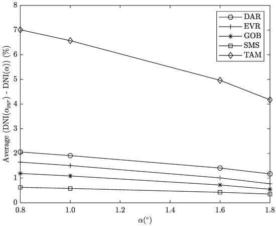
Figure 1.
Average difference between and .
The average difference between and is higher for lower half-opening angles as expected, and for locations with higher CSR. The locations with higher average difference are TAM and DAR, whilst locations such as GOB and SMS show low average differences between the DNI of the pyrheliometer and the DNI for lower half-opening angles. This is related to the CSR magnitude across different locations, and in turn, with the composition of the atmosphere, in particular with the type and concentration of aerosols. It is worth mentioning that not only the magnitude of the average difference across locations depends on the composition of the atmosphere, but also the slope of the lines shown in Figure 1. Locations with higher aerosol concentration have higher slopes (e.g., TAM) as can be seen in Figure 2, where boxplots for aerosol optical depth (AOD) and single scattering albedo (SSA) at 675 nm are shown. Figure 1 and Figure 2 highlight the need for the consideration of both the half-opening aperture angle and the CSNI when designing and simulating CSP systems, especially in locations with higher aerosol concentration. Differences in the incoming DNI of around 7% and 2% for locations such as TAM and DAR, respectively, can lead to erroneous energy generation estimates, which in turn can jeopardize the economic viability of the CSP projects.
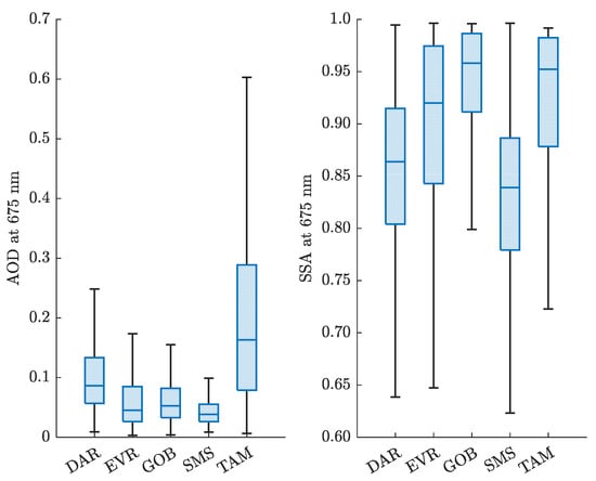
Figure 2.
Boxplots for aerosol optical depth (AOD) and single scattering albedo (SSA) for the stations analyzed in this work.
4.2. Impact on the Intercept Factor of CSP Systems: The Case of Parabolic trough Concentrators
The model from Bendt et al. [14] was used here to quantify in a simple way the impact of CSR in the optical efficiency of a parabolic trough CSP system with cylindrical receiver.
In that work [14], an analytical approach was proposed to perform the optical analysis of a solar concentrator instead of using ray-tracing software. The former approach is simpler and faster than the later, hence it was used here. By assuming a Gaussian distribution for the sun shape, Bendt et al. [14] were able to determine the intercept factor (the ratio of the irradiance reaching the receiver over the incident irradiance) as a function of the group , where σ stands for total optical error and C for concentration ratio.
To achieve this, the model by Bendt et al. [14] determines an effective source that accounts for the shape of the sun, and for all optical errors from the parabolic trough system. In this way, it is possible to determine the intercept factor.
The total optical error () is defined as the root mean square of angular spread caused by all optical errors of the concentrator () and the angular width of the sun shape in line focus geometry (), through the following equation:
To study the impact of CSNI (or CSR) variation on CSP systems, namely, parabolic trough systems, a relationship between and CSR was established using data from Table 4-1 in Bendt et al. [14]. This table contains data from the 16 standard Lawrence Berkeley Laboratory (LBL) circumsolar irradiance scans [26], namely, and CSR, and its relationship is shown in Figure 3.
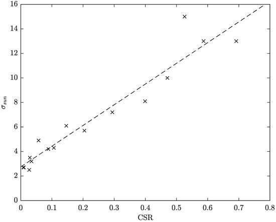
Figure 3.
Relationship between CSR and .
Then, a fit to the data shown in Figure 4–1a of Bendt et al. [14] was performed, enabling the determination of the intercept factor according to CSR using the procedure described below. Firstly, was fixed at 10 mrad and varied from 2.5 mrad to 10 mrad. In this way, it was possible to determine the intercept factor for various combinations of concentration factors (C) and rim angles, as shown in Figure 4 for a given parabolic trough system.
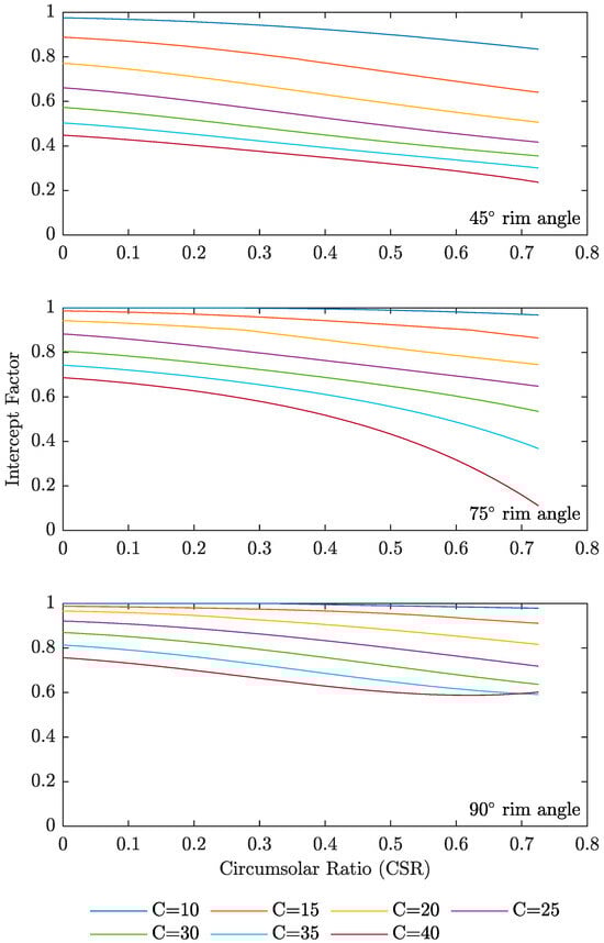
Figure 4.
Variation of intercept factor according to CSR for a parabolic trough system with rim angle of 45° (top), 75° (middle), and 90° (bottom).
From Figure 4, it is clear that higher concentration ratios imply a larger effect of the CSR on the intercept factor of a parabolic trough system, regardless of the selected rim angle. Higher CSR values stand for higher dispersion of reflected solar rays from the parabolic through the concentrator to the receiver, resulting in a lower intercept factor.
For lower rim angles, the CSR seems to have a larger impact on the intercept factor than for higher rim angles, for the same concentration ratio. This has to do with the aperture angle of the reflector, because lower rim angles correspond to lower acceptance angles of the reflector. Therefore, lower reflector aperture angles result in less irradiance reflected when the circumsolar region is larger (i.e., higher CSR).
Regarding the mitigation of CSR effects on the intercept factor of parabolic trough systems, it appears that using higher rim angles is the best approach based on the results from Figure 4. It is expected that the same conclusions could be draw for other CSP systems. For instance, Rabl and Bendt [27] found that the intercept factor of a parabolic dish strongly depended on the rim angle. They also stated that concentrators with a rim angle of 30º are two times more sensitive to CSNI variation than those with a rim angle of 60º. However, those systems are not addressed here for conciseness.
5. Conclusions
In this work, a model to predict circumsolar normal irradiance (CSNI) for several half-opening angles was developed. The model is based on the CSR model developed by Abreu et al. [6] and uses a polynomial fitting of the model parameters to estimate CSNI for half-opening angles of interest for CSP systems, such as parabolic trough and parabolic disk. It was found that the proposed model performs significantly better at the locations under study here than the other models available in the literature. It was also found that the local aerosol regime and atmospheric conditions have a higher impact on model fitting and performance than the overall climate zone of the locations under study.
Regarding the impact of CSNI in CSP systems, it was found that discarding an accurate CSNI estimate could lead to up to a 7% difference between the DNI that is measured by a pyrheliometer and the DNI that is effectively captured by the system. It was also found that these differences are greater for lower half-opening angles, as expected, since the difference between the half-opening angle of the pyrheliometer and the half-opening angle of the CSP system is greater.
The impact of CSNI in the operation of a CSP system, namely with parabolic trough concentrators, was also studied in this work. The authors found that higher CSR values lead to lower intercept factors (the ratio between the irradiance reaching the receiver over the incident irradiance) for these systems. It was also found that if parabolic trough designers aim to reduce the impact of CSNI on the intercept factor, then parabolic troughs with higher rim angles are preferred.
This study also found that further study on the direct impact of the different aerosol and atmospheric characteristics on the development of local or global CSNI models, as well as on the evaluation of the impact of CSNI in other CSP systems, is needed and should be addressed in future work.
Author Contributions
Conceptualization, E.F.M.A., P.C. and M.J.C.; Methodology, E.F.M.A. and P.C.; validation, E.F.M.A.; writing—original draft preparation, E.F.M.A.; writing—review and editing, P.C. and M.J.C.; supervision, P.C. and M.J.C. All authors have read and agreed to the published version of the manuscript.
Funding
This research was funded by FCT (the Portuguese Science and Technology Foundation), grant number SFRH/BD/136433/2018, co-funded by National funds through FCT—Fundação para a Ciência e Tecnologia, I.P., projects UIDB/04683/2020 and UIDP/04683/2020, and it was also funded by the European Union through the European Regional Development Fund, included in the COMPETE 2020 (Operational Program Competitiveness and Internationalization) through the project DNI-Alentejo with reference ALT20-03-0145-FEDER-000011. The APC was funded by the Institute of Earth Sciences.
Data Availability Statement
The data presented in this study are available on request from the corresponding author.
Conflicts of Interest
The authors declare no conflict of interest. The funders had no role in the design of the study; in the collection, analyses, or interpretation of data; in the writing of the manuscript; or in the decision to publish the results.
Appendix A
Table A1.
Statistical analysis of circumsolar models for a half-opening value of 1.0°. Legend: TR—Tropical; TM—Temperate; AR—Arid. Values in bold indicate the best performing model according to each statistical indicator.
Table A1.
Statistical analysis of circumsolar models for a half-opening value of 1.0°. Legend: TR—Tropical; TM—Temperate; AR—Arid. Values in bold indicate the best performing model according to each statistical indicator.
| Station | Statistical Indicator | Models | |||
|---|---|---|---|---|---|
| Eissa et al. [5] SOV | Eissa et al. [5] TAM | Eissa et al. [5] Combined | This Work | ||
| DAR (TR) | rMBE (%) | −8.28 | −16.53 | −12.94 | −2.25 |
| rRMSE (%) | 74.34 | 76.38 | 75.23 | 64.85 | |
| R | 0.4616 | 0.4516 | 0.4585 | 0.6277 | |
| FB | 0.0647 | −0.0137 | 0.0180 | 0.0694 | |
| FGE | 0.3966 | 0.3979 | 0.3946 | 0.3282 | |
| EVR (TM) | rMBE (%) | −17.47 | −24.30 | −21.61 | −4.13 |
| rRMSE (%) | 68.06 | 72.60 | 70.28 | 48.07 | |
| R | 0.7515 | 0.7475 | 0.7506 | 0.8641 | |
| FB | 0.0549 | −0.0116 | 0.0084 | 0.0634 | |
| FGE | 0.4575 | 0.4660 | 0.4577 | 0.3657 | |
| SMS (TM) | rMBE (%) | 51.23 | 41.23 | 44.25 | −7.88 |
| rRMSE (%) | 94.91 | 87.53 | 90.03 | 59.32 | |
| R | 0.5944 | 0.5952 | 0.5963 | 0.7761 | |
| FB | 0.5935 | 0.5399 | 0.5512 | −0.0536 | |
| FGE | 0.6657 | 0.6321 | 0.6352 | 0.4101 | |
| GOB (AR) | rMBE (%) | −9.66 | −16.54 | −13.97 | 0.40 |
| rRMSE (%) | 76.16 | 78.58 | 77.29 | 63.26 | |
| R | 0.5963 | 0.5905 | 0.5950 | 0.7356 | |
| FB | 0.1261 | 0.0626 | 0.0812 | 0.1404 | |
| FGE | 0.4574 | 0.4542 | 0.4506 | 0.4007 | |
| TAM (AR) | rMBE (%) | −46.42 | −51.60 | −49.26 | −11.08 |
| rRMSE (%) | 64.19 | 68.52 | 66.48 | 35.98 | |
| R | 0.6587 | 0.6591 | 0.6596 | 0.8105 | |
| FB | −0.6053 | −0.6832 | −0.6521 | −0.0800 | |
| FGE | 0.6179 | 0.6882 | 0.6597 | 0.2596 | |
Table A2.
Statistical analysis of circumsolar models for a half-opening value of 1.6°. Legend: TR—Tropical; TM—Temperate; AR—Arid. Values in bold indicate the best performing model according to each statistical indicator.
Table A2.
Statistical analysis of circumsolar models for a half-opening value of 1.6°. Legend: TR—Tropical; TM—Temperate; AR—Arid. Values in bold indicate the best performing model according to each statistical indicator.
| Station | Statistical Indicator | Models | |||
|---|---|---|---|---|---|
| Eissa et al. [5] SOV | Eissa et al. [5] TAM | Eissa et al. [5] Combined | This Work | ||
| DAR (TR) | rMBE (%) | −7.32 | −14.46 | −11.38 | −2.97 |
| rRMSE (%) | 71.52 | 73.24 | 72.26 | 61.41 | |
| R | 0.4884 | 0.4792 | 0.4856 | 0.6585 | |
| FB | 0.0677 | −0.0004 | 0.0262 | 0.0495 | |
| FGE | 0.3861 | 0.3865 | 0.3836 | 0.3096 | |
| EVR (TM) | rMBE (%) | −18.22 | −24.22 | −21.90 | −6.00 |
| rRMSE (%) | 69.00 | 73.07 | 70.96 | 47.49 | |
| R | 0.7651 | 0.7615 | 0.7644 | 0.8773 | |
| FB | 0.0501 | −0.0126 | 0.0050 | 0.0379 | |
| FGE | 0.4479 | 0.4538 | 0.4470 | 0.3495 | |
| SMS (TM) | rMBE (%) | 55.71 | 46.30 | 48.97 | −8.79 |
| rRMSE (%) | 97.65 | 90.25 | 92.75 | 58.16 | |
| R | 0.6026 | 0.6060 | 0.6058 | 0.7872 | |
| FB | 0.6128 | 0.5599 | 0.5702 | −0.0604 | |
| FGE | 0.6748 | 0.6359 | 0.6409 | 0.3856 | |
| GOB (AR) | rMBE (%) | −9.47 | −15.53 | −13.34 | 0.35 |
| rRMSE (%) | 74.01 | 76.00 | 74.93 | 60.11 | |
| R | 0.6099 | 0.6058 | 0.6095 | 0.7565 | |
| FB | 0.1208 | 0.0614 | 0.0776 | 0.1306 | |
| FGE | 0.4457 | 0.4389 | 0.4367 | 0.3819 | |
| TAM (AR) | rMBE (%) | −47.77 | −52.19 | −50.16 | −13.12 |
| rRMSE (%) | 65.61 | 69.38 | 67.56 | 36.73 | |
| R | 0.6736 | 0.6744 | 0.6748 | 0.8230 | |
| FB | −0.6253 | −0.6952 | −0.6679 | −0.1024 | |
| FGE | 0.6334 | 0.6981 | 0.6728 | 0.2593 | |
Table A3.
Statistical analysis of circumsolar models for a half-opening value of 1.8°. Legend: TR—Tropical; TM—Temperate; AR—Arid. Values in bold indicate the best performing model according to each statistical indicator.
Table A3.
Statistical analysis of circumsolar models for a half-opening value of 1.8°. Legend: TR—Tropical; TM—Temperate; AR—Arid. Values in bold indicate the best performing model according to each statistical indicator.
| Station | Statistical Indicator | Models | |||
|---|---|---|---|---|---|
| Eissa et al. [5] SOV | Eissa et al. [5] TAM | Eissa et al. [5] Combined | This Work | ||
| DAR (TR) | rMBE (%) | −11.28 | −17.81 | −15.01 | −3.11 |
| rRMSE (%) | 69.47 | 71.49 | 70.39 | 58.15 | |
| R | 0.5053 | 0.4969 | 0.5029 | 0.6813 | |
| FB | 0.0232 | −0.0431 | −0.0176 | 0.0445 | |
| FGE | 0.3809 | 0.3856 | 0.3815 | 0.3012 | |
| EVR (TM) | rMBE (%) | −22.25 | −27.84 | −25.70 | −6.46 |
| rRMSE (%) | 70.11 | 74.19 | 72.10 | 46.61 | |
| R | 0.7747 | 0.7717 | 0.7744 | 0.8822 | |
| FB | 0.0009 | −0.0634 | −0.0456 | 0.0261 | |
| FGE | 0.4434 | 0.4518 | 0.4445 | 0.3420 | |
| SMS (TM) | rMBE (%) | 50.25 | 41.06 | 43.62 | −8.91 |
| rRMSE (%) | 92.84 | 86.01 | 88.31 | 56.76 | |
| R | 0.6065 | 0.6118 | 0.6106 | 0.7919 | |
| FB | 0.5766 | 0.5198 | 0.5312 | −0.0668 | |
| FGE | 0.6454 | 0.6036 | 0.6094 | 0.3789 | |
| GOB (AR) | rMBE (%) | −13.74 | −19.40 | −17.39 | 0.01 |
| rRMSE (%) | 74.10 | 76.24 | 75.14 | 59.07 | |
| R | 0.6138 | 0.6110 | 0.6140 | 0.7617 | |
| FB | 0.0719 | 0.0109 | 0.0273 | 0.1230 | |
| FGE | 0.4310 | 0.4270 | 0.4244 | 0.3730 | |
| TAM (AR) | rMBE (%) | −50.66 | −54.66 | −52.82 | −13.94 |
| rRMSE (%) | 68.04 | 71.56 | 69.85 | 37.16 | |
| R | 0.6778 | 0.6787 | 0.6792 | 0.8243 | |
| FB | −0.6735 | −0.7412 | −0.7149 | −0.1121 | |
| FGE | 0.6772 | 0.7426 | 0.7171 | 0.2589 | |
References
- Polo, J.; Fernández-Peruchena, C.; Gastón, M. Analysis on the Long-Term Relationship between DNI and CSP Yield Production for Different Technologies. Sol. Energy 2017, 155, 1121–1129. [Google Scholar] [CrossRef]
- Blanc, P.; Espinar, B.; Geuder, N.; Gueymard, C.; Meyer, R.; Pitz-Paal, R.; Reinhardt, B.; Renné, D.; Sengupta, M.; Wald, L.; et al. Direct Normal Irradiance Related Definitions and Applications: The Circumsolar Issue. Sol. Energy 2014, 110, 561–577. [Google Scholar] [CrossRef]
- World Meteorological Organization (WMO). Guide to Instruments and Methods of Observation. Volume I—Measurement of Meteorological Variables; World Meteorological Organization (WMO): Geneva, Switzerland, 2021. [Google Scholar]
- Rabl, A. Comparison of Solar Concentrators. Sol. Energy 1976, 18, 93–111. [Google Scholar] [CrossRef]
- Eissa, Y.; Blanc, P.; Ghedira, H.; Oumbe, A.; Wald, L. A Fast and Simple Model to Estimate the Contribution of the Circumsolar Irradiance to Measured Broadband Beam Irradiance under Cloud-Free Conditions in Desert Environment. Sol. Energy 2018, 163, 497–509. [Google Scholar] [CrossRef]
- Abreu, E.F.M.; Canhoto, P.; Costa, M.J. Development of a Clear-Sky Model to Determine Circumsolar Irradiance Using Widely Available Solar Radiation Data. Sol. Energy 2020, 205, 88–101. [Google Scholar] [CrossRef]
- Abreu, E.F.M.; Canhoto, P.; Costa, M.J. Circumsolar Irradiance Modelling Using libRadtran and AERONET Data. AIP Conf. Proc. 2019, 2126, 190001. [Google Scholar]
- Mayer, B.; Kylling, A. Technical Note: The libRadtran Software Package for Radiative Transfer Calculations—Description and Examples of Use. Atmos. Chem. Phys. 2005, 23, 1855–1877. [Google Scholar] [CrossRef]
- Ivanova, S.M. Modelling of Circumsolar Direct Irradiance as a Function of GHI, DHI and DNI. In Proceedings of the 8th International Conference on Solar Radiation and Daylighting Solaris-2017, London, UK, 27–28 July 2017. [Google Scholar]
- Neumann, A.; von der Au, B.; Heller, P. Measurements of Circumsolar Radiation at the Plataforma Solar (Spain) and at DLR (Germany); ASME International Solar Energy Conference: Albuquerque, NM, USA, 1998; pp. 429–438. [Google Scholar]
- Forman, P.; Penkert, S.; Kämper, C.; Stallmann, T.; Mark, P.; Schnell, J. A Survey of Solar Concrete Shell Collectors for Parabolic Troughs. Renew. Sustain. Energy Rev. 2020, 134, 110331. [Google Scholar] [CrossRef]
- Belhomme, B.; Pitz-Paal, R.; Schwarzbözl, P.; Ulmer, S. A New Fast Ray Tracing Tool for High-Precision Simulation of Heliostat Fields. J. Sol. Energy Eng. 2009, 131, 031002. [Google Scholar] [CrossRef]
- Leary, P.L.; Hankins, J.D. User’s Guide for MIRVAL: A Computer Code for Comparing Designs of Heliostat-Receiver Optics for Central Receiver Solar Power Plants; Sandia National Lab. (SNL-CA): Livermore, CA, USA, 1979. [Google Scholar]
- Bendt, P.; Rabl, A.; Gaul, H.W.; Reed, K.A. Optical Analysis and Optimization of Line Focus Solar Collectors; Solar Energy Research Institution: Golden, CO, USA, 1979. [Google Scholar]
- Schwarzbözl, P.; Pitz-Paal, R.; Schmitz, M. Visual HFLCAL—A Software Tool for Layout and Optimisation of Heliostat Fields. In Proceedings of the SolarPACES 2009, Berlin, Germany, 15–18 September 2009. [Google Scholar]
- Gilman, P.; Blair, N.; Mehos, M.; Christensen, C.; Janzou, S.; Cameron, C. Solar Advisor Model User Guide for Version 2.0; National Renewable Energy Laboratory: Colorado, CO, USA, 2008; NREL/TP-670-43704, 937349. [Google Scholar]
- Quaschning, V.; Ortmanns, W.; Kistner, R.; Geyer, M. Greenius: A New Simulation Environment for Technical and Economical Analysis of Renewable Independent Power Projects. In Proceedings of the SED2001, Solar Engineering 2001: (FORUM 2001: Solar Energy—The Power to Choose), Washington, DC, USA, 21 April 2001; pp. 413–417. [Google Scholar]
- Dersch, J.; Schwarzbözl, P.; Richert, T. Annual Yield Analysis of Solar Tower Power Plants With GREENIUS. J. Sol. Energy Eng. 2011, 133, 031017. [Google Scholar] [CrossRef]
- Holben, B.N.; Eck, T.F.; Slutsker, I.; Tanré, D.; Buis, J.P.; Setzer, A.; Vermote, E.; Reagan, J.A.; Kaufman, Y.J.; Nakajima, T.; et al. AERONET—A Federated Instrument Network and Data Archive for Aerosol Characterization. Remote Sens. Environ. 1998, 66, 1–16. [Google Scholar] [CrossRef]
- Driemel, A.; Augustine, J.; Behrens, K.; Colle, S.; Cox, C.; Cuevas-Agulló, E.; Denn, F.M.; Duprat, T.; Fukuda, M.; Grobe, H.; et al. Baseline Surface Radiation Network (BSRN): Structure and Data description (1992–2017). Earth Syst. Sci. Data 2018, 10, 1491–1501. [Google Scholar] [CrossRef]
- Giles, D.M.; Sinyuk, A.; Sorokin, M.G.; Schafer, J.S.; Smirnov, A.; Slutsker, I.; Eck, T.F.; Holben, B.N.; Lewis, J.R.; Campbell, J.R.; et al. Advancements in the Aerosol Robotic Network (AERONET) Version 3 Database—Automated near-Real-Time Quality Control Algorithm with Improved Cloud Screening for Sun Photometer Aerosol Optical Depth (AOD) Measurements. Atmos. Meas. Tech. 2019, 12, 169–209. [Google Scholar] [CrossRef]
- Sinyuk, A.; Holben, B.N.; Eck, T.F.; Giles, D.M.; Slutsker, I.; Korkin, S.; Schafer, J.S.; Smirnov, A.; Sorokin, M.; Lyapustin, A. The AERONET Version 3 Aerosol Retrieval Algorithm, Associated Uncertainties and Comparisons to Version 2. Atmos. Meas. Tech. 2020, 13, 3375–3411. [Google Scholar] [CrossRef]
- Liu, B.Y.H.; Jordan, R.C. The Interrelationship and Characteristic Distribution of Direct, Diffuse and Total Solar Radiation. Sol. Energy 1960, 4, 1–19. [Google Scholar] [CrossRef]
- Gueymard, C.A.; Ruiz-Arias, J.A. Extensive Worldwide Validation and Climate Sensitivity Analysis of Direct Irradiance Predictions from 1-Min Global Irradiance. Sol. Energy 2016, 128, 1–30. [Google Scholar] [CrossRef]
- Gueymard, C.A.; Bright, J.M.; Lingfors, D.; Habte, A.; Sengupta, M. A Posteriori Clear-Sky Identification Methods in Solar Irradiance Time Series: Review and Preliminary Validation Using Sky Imagers. Renew. Sustain. Energy Rev. 2019, 109, 412–427. [Google Scholar] [CrossRef]
- Noring, J.E.; Grether, D.F.; Hunt, A.J. Circumsolar Radiation Data: The Lawrence Berkeley Laboratory Reduced Data Base. NASA STI/Recon Tech. Rep. N 1991, 92, 19628. [Google Scholar]
- Rabl, A.; Bendt, P. Effect of Circumsolar Radiation on Performance of Focusing Collectors. J. Sol. Energy Eng. 1982, 104, 237–250. [Google Scholar] [CrossRef]
Disclaimer/Publisher’s Note: The statements, opinions and data contained in all publications are solely those of the individual author(s) and contributor(s) and not of MDPI and/or the editor(s). MDPI and/or the editor(s) disclaim responsibility for any injury to people or property resulting from any ideas, methods, instructions or products referred to in the content. |
© 2023 by the authors. Licensee MDPI, Basel, Switzerland. This article is an open access article distributed under the terms and conditions of the Creative Commons Attribution (CC BY) license (https://creativecommons.org/licenses/by/4.0/).