Abstract
The electricity consumption behavior of the inhabitants is a major contributor to the uncertainty of the residential load system. Human-caused uncertainty may have a distributional component, but it is not well understood, which limits further understanding the stochastic component of load forecasting. This study proposes a short-term load-interval forecasting method considering the stochastic features caused by users’ electricity consumption behavior. The proposed method is composed of two parts: load-point forecasting using singular spectrum analysis and long short-term memory (SSA-LSTM), and load boundaries forecasting using statistical analysis. Firstly, the load sequence is decomposed and recombined using SSA to obtain regular and stochastic subsequences. Then, the load-point forecasting LSTM network model is trained from the regular subsequence. Subsequently, the load boundaries related to load consumption consistency are forecasted by statistical analysis. Finally, the forecasting results are combined to obtain the load-interval forecasting result. The case study reveals that compared with other common methods, the proposed method can forecast the load interval more accurately and stably based on the load time series. By using the proposed method, the evaluation index coverage rates (CRs) are (17.50%, 1.95%, 1.05%, 0.97%, 7.80%, 4.55%, 9.52%, 1.11%), (17.95%, 3.02%, 1.49%, 5.49%, 5.03%, 1.66%, 1.49%), (19.79%, 2.79%, 1.43%, 1.18%, 3.37%, 1.42%) higher than the compared methods, and the interval average convergences (IACs) are (−18.19%, −8.15%, 3.97%), (36.97%, 21.92%, 22.59%), (12.31%, 21.59%, 7.22%) compared to the existing methods in three different counties, respectively, which shows that the proposed method has better overall performance and applicability through our discussion.
1. Introduction
Short-term load forecasting refers to forecasting load data for a several-hour period. The residential load side plays an important role in the supply and demand interaction in the power system [1]. Regional residential load forecasting is crucial for safety management, regulation, and scheduling in the power system, as well as for lowering costs and improving efficiency [2,3,4,5]. The daily, weekly, and annual consistency of various residents’ power consumption contributes to the regular component of the load data since the residential load is produced by the daily activities of residents. Additionally, different customs and behaviors of residents will produce inconsistent load consumption, resulting in stochastic features in the load. These stochastic features will cause fluctuations in the load time series and make load forecasting more challenging. In general, the regular component can be analyzed through the nonlinear fitting method, while the stochastic part can be analyzed by a statistical distribution. As a result, load forecasting that takes into account both the regular component and the stochastic features will be more accurate and useful for the power system.
Regarding the load regular component, many studies have used load-point forecasting to capture the features. Artificial intelligence (AI)-based methods including extreme learning machines (ELM) [6], neural networks (NN) [7], and random forests (RF) [8] are frequently used to increase the accuracy in load forecasting. Deep learning algorithms have demonstrated their advantages in long sequence dependence problems (for example, electricity load) and can deal with historical data successfully [9]. Long short–term memory (LSTM) is one of the variants of deep learning and has shown superior performance to other algorithms in specific load forecasting scenarios. The LSTM model built in [10] proves that the LSTM-based load forecast performs better than some machine learning methods like radial basis function network and extreme gradient boosting algorithm. Another LSTM model built in [11] also shows advantages compared to conventional methods. In general, load-point forecasting can determine the load trend and provide a relatively more accurate forecasting result. However, load-point forecasting may result in information loss due to the high degree of randomness in the residential load data on a short-term scale [12]. Load-interval forecasting, which means forecasting the upper bound and lower bound of the load, has the potential to contain both the load-point forecasting results and the load uncertainty information [13]. Thus, the issue with load series uncertainties can be resolved by the combination of load-point forecasting and load boundary analysis.
The load uncertainties caused by load consumption consistency features have been widely researched. The load uncertain consumption behavior while using an energy storage system is researched in [14], which shows that the load consumption consistency will affect the energy scheduling. In literature [15], MA Judge et al. analyzed load uncertainties caused by interruptible loads and thermostatically controlled loads’ use and controlled demand size through robust optimization. Numerous studies on the modeling of the impact of inconsistencies on load were conducted by researchers to deepen their understanding of the uncertainties. In literature [16], S Teshnehdel et al. studied 10 traditional courtyards located in warm-dry climates of Kashan and cold climates of Ardabil based on shading and sunlit coverage and built a model of the load consumption behavior of users in various weather scenarios. In literature [17], NS Pearre et al. conducted research on grid-embedded devices and confirmed that user energy consumption behavior would be affected by new grid-embedded power equipment using statistical analysis. In load forecasting fields, scholars have also noted the human behavior-related uncertainty in electricity consumption and carried out research on related issues. Additionally, data decomposition–recombination techniques such as empirical mode decomposition (EMD), singular spectrum analysis (SSA), and wavelet transformation (WT) were used to obtain different components in the load time series. In literature [18], M Anvari et al. studied residential load data from Austria, Germany, and the United Kingdom, analyzed load data based on empirical mode decomposition (EMD), and then applied a stochastic model to quantify demand fluctuations in load sequence. In literature [13], D Yang et al. extracted different components in data using bivariate empirical mode decomposition (BEMD) and realized load-interval forecasting by component reorganization and forecasting reconstruction process. In literature [19], Y Wang et al. built a line regression model for the trend series and an XGBoost regression model for each fluctuation sub-series in the decomposed load data and the model showed improved performance over the contrast models in state-of-the-art load forecasting. However, the current uncertainty research in load forecasting is largely focused on the examination of the load data themselves [20,21,22], and there is still a lack of research on the connection between the modeling of the impact of inconsistencies on load and the uncertainties in electricity consumption. In other words, the mapping between consistency features of load consumption and load uncertainties is not studied enough.
To sum up, although current research has used different algorithms and methods to build load-interval forecasting models, there are still limitations in the related research. First, the features of residents’ load consumption have not been completely studied. The load time series consists of load trend information and load fluctuation information, but only a few researchers have conducted relevant studies. Second, in the research, the relationship between users’ electricity consumption consistency behavior and the load feature has not been introduced into load forecasting research. Third, the current research mainly obtains load-interval data by grouping the load time series, so there is a need to find a way to convert a time series into a time interval series without loss of accuracy.
In conclusion, a behavioral explanation is lacking in the present research on load-interval forecasting, which prevents the advancement of more precise and explicable forecasting. To explore the solutions to these problems, the distribution analysis of load stochastic subsequence is introduced as the foundation of load boundary forecasting, and a load-interval forecasting model that incorporates both the regular part and the stochastic features is proposed in this paper. First, the residential load sequence is decomposed into subsequences by SSA, and the subsequences are recombined into regular subsequences and stochastic subsequences. Then, the load-point forecasting model is built with the regular subsequence based on LSTM. Second, based on the diversity factor (DF), an indicator that reflects the electricity consumption consistency of regional users, the mapping from user behavior to load boundaries is developed so that the method to obtain load-interval data from load consumption consistency can be realized. Third, the load-interval forecasting result is obtained by combining the short-term load-point forecasting model and the load boundary analysis. Finally, the case study is carried out to verify the performance of the proposed method. Compared with the existing methods, the features of our proposed load forecasting method are as below:
- (1)
- The load data are divided into the regular part and the random part by SSA, that is, the long-term residents’ load consumption trend and the short-term load consumption fluctuation;
- (2)
- The trend and randomness of user electricity consumption are analyzed and forecasted separately and then combined to improve the accuracy and interpretability of the forecasting result;
- (3)
- The relationship between regional residents’ load consumption consistency and user behavior is studied, and a statistical correlation is constructed from residents’ load consumption behavior to load consumption fluctuation characteristics;
- (4)
- A load-interval forecasting method is constructed based on one-dimensional regional load time series.
The rest of this paper is arranged as follows: the methodology and modeling framework for constructing the short-term load-interval forecasting model is introduced in Section 2. The case study and forecasting results are presented in Section 3. The necessary discussion about the results and comparisons are discussed in Section 4. The conclusion of the paper and the feasible further research are shown in Section 5.
2. Materials and Methods
2.1. Load-point forecasting Based on SSA-LSTM
The regular subsequence of the original load sequence can be forecasted with an LSTM network in the proposed method. The input includes load regular subsequence data and temperature data.
2.1.1. Singular Spectrum Analysis
In the proposed load-interval forecasting method, the load time series needs to be first decomposed and recombined into the regular subsequence and the stochastic subsequence, which represent the load consumption consistency and inconsistency of humans, respectively.
Singular spectrum analysis (SSA) [23] is a non-parametric method used to analyze nonlinear time sequence data. SSA constructs a trajectory matrix based on the original time sequence and then decomposes and recombines the trajectory matrix, thereby extracting subsequences representing different characteristics of the original time series [24], such as trend subsequence, periodic subsequence, noise subsequence, etc., to analyze the composition of the original sequence. As for the regional residential electricity load sequence , the SSA process is as follows:
(1) Embedding. For the load sequence, let the embedding dimension L be an integer and satisfy , where n represents the length of the load sequence. Then a delay vector can be defined as , from which a trajectory matrix X consisting of K delay vectors can be reconstructed:
where , the trajectory matrix X is a Hankel matrix and can be restored to the original sequence after the diagonal averaging process, in which the column vector and row vector are both subsets of the original sequence .
(2) SVD. Calculate , and perform SVD on the result to obtain L non-negative eigenvalues (in descending order) and their corresponding orthogonal eigenvectors . Let d equal the number of non-zero eigenvalues, then the trajectory matrix X in Step (1) can be expressed as follows:
where represents eigenvalues of X, is the singular spectrum, is usually represented by the empirical orthogonal functions (EOF), is the principal components (PC), represents the triple eigenvector of X.
(3) Grouping. Keep the first r in step (2) to obtain an approximate matrix X and divide X into p groups. Suppose there are matrices in the group, add up the matrices in each group to obtain new matrices , then the trajectory matrix X can be approximately presented as follows:
where the contribution rate of is .
(4) Diagonal averaging. Revert matrix to time series. Let the elements in be , , , then the process during which can be converted into the corresponding time sequence can be obtained as follows:
there will be d reconstructed sequences after converting the sub-matrix in step (2).
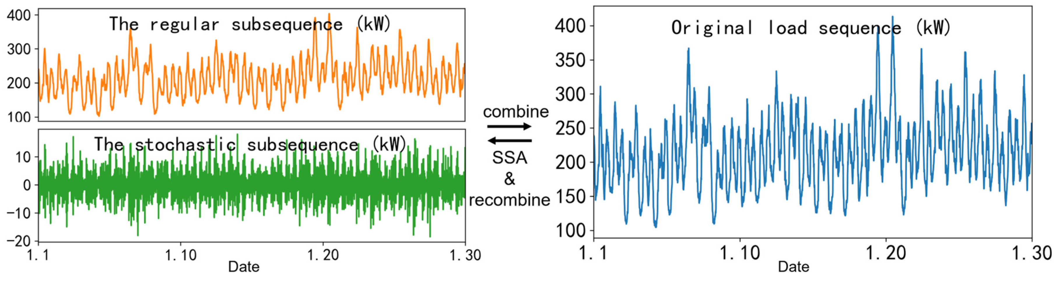
In this paper, all the subsequences are split into two groups and recombined by adding up the subsequences, and Figure 1 shows the two recombined subsequences. The first recombined subsequence (the regular subsequence) is used as the input of the LSTM network to build the load-point forecasting model. The second subsequence (the stochastic subsequence) is used for statistical analysis and the subsequent mapping of load consumption consistency to load fluctuations.
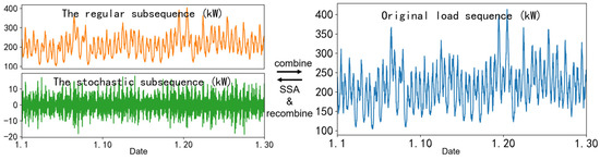
Figure 1.
The regular subsequence and the stochastic subsequence of the load sequence.
2.1.2. Long Short-Term Memory Network
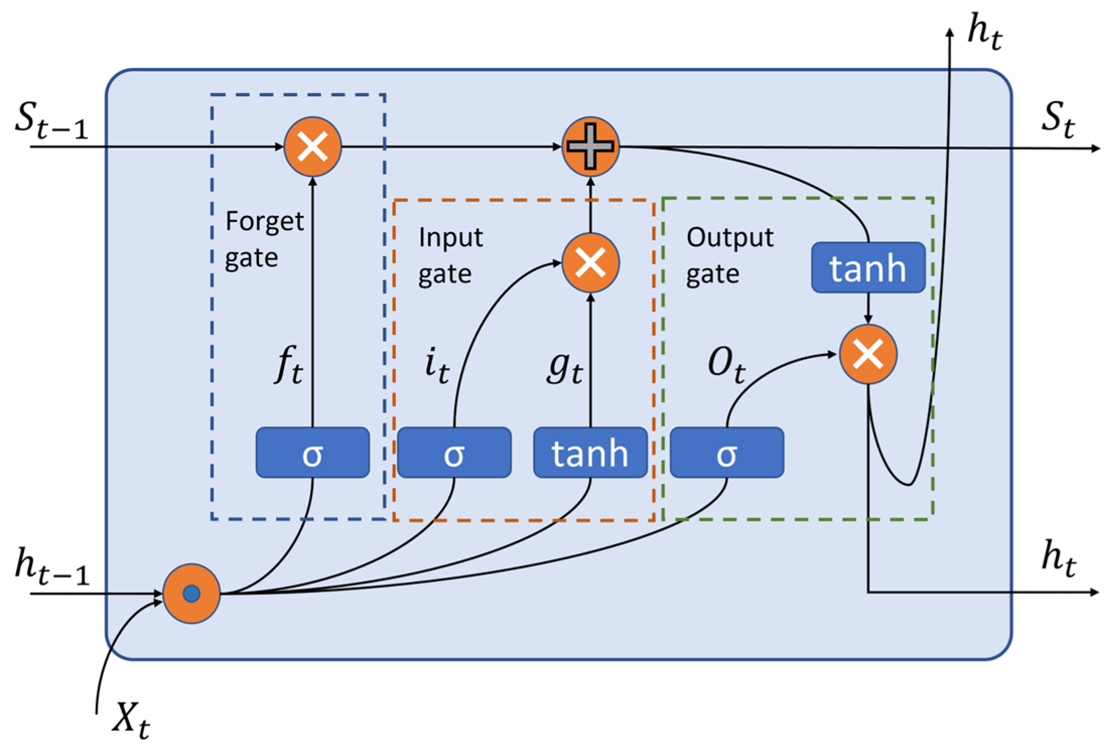
Long short-term memory (LSTM) is a special kind of RNN model [25] which can effectively record information on long-term input features. In the load forecasting model built by the LSTM network, several layers of repetitive LSTM memory cells are included. The structure of the memory cells in the LSTM network is shown in Figure 2. The LSTM cells include the forget gate, the input gate, and the output gate, and the cells can play the role of information memory or forgetting in the neural network.

Figure 2.
The structure of LSTM cells.
This paper defines the input of LSTM network , where represents the historical electric load data from the SSA recombined process and represents the corresponding historical temperature data, then the information processing process of the LSTM cells can be constructed as follows:
where and is the output and state of the previous LSTM cell at the previous moment, respectively, , and represents the output, state, and input of the LSTM cell at the current moment, respectively. The different represents different weight matrices and the different represents different bias matrices. and represent the sigmoid network layer and the tanh network layer.
This paper builds the short-term load-point forecasting model based on the LSTM network. The load forecasting model is obtained by training the model using the SSA recombined regular subsequence and other relevant inputs.
2.1.3. Subsequences Recombination
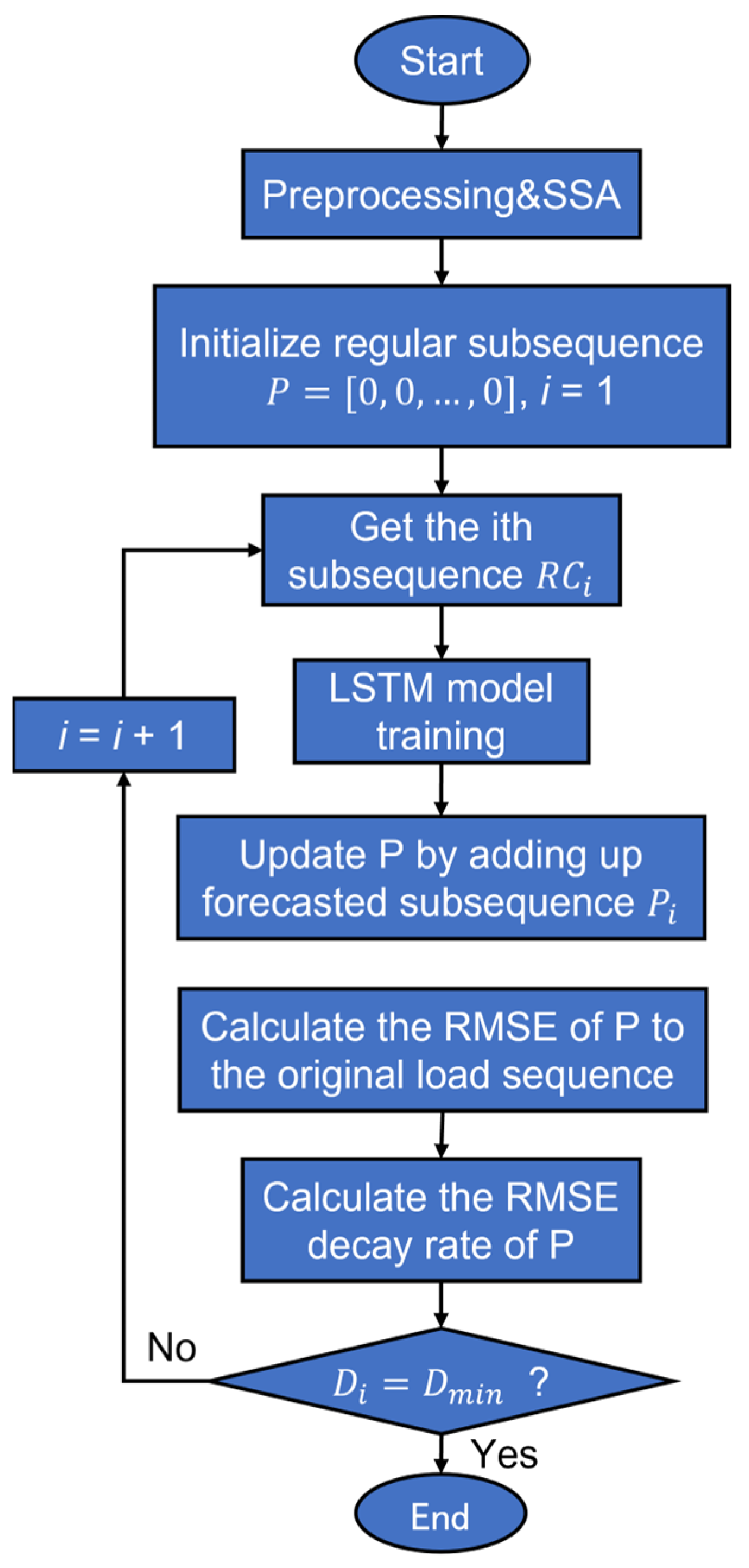
To obtain the most suitable regular subsequence that fully reflects the features of the original load time series, the number of subsequences that should be forecasted and recombined to the regular subsequence needs to be determined. If too many subsequences are used for recombination, the LSTM forecasting network will be hard to train, and overfitting may occur. If too few subsequences are used, the main sequence cannot reproduce the original load sequence very well, and the calculation on load fluctuation, that is, the stochastic subsequence, will be not accurate enough.
To obtain , this paper uses root mean square error (RMSE) to calculate the error between the forecasting regular sequence after recombination and the original load sequence. The RMSE can measure the average size of the error, which is the square root of the average value of the squared difference between the forecasting sequence and the real sequence:
where N represents the length of the load sequence, represents the forecasting regular sequence, and represents the real load. The flowchart of the recombination process can be seen in Figure 3. Considering the time cost of model training and the requirement of model forecasting accuracy, this paper takes 1% as the threshold of the RMSE decay rate.

Figure 3.
The flowchart of the subsequences recombination process.
2.2. Load Boundaries Forecasting Based on Statistical Distribution and Load Consumption Consistency
The point forecasting model on the regular subsequence based on SSA-LSTM can provide relatively accurate forecasting results, but the stochastic subsequence obtained from the SSA process still needs to be analyzed. This stochastic subsequence with stochastic characteristics is mainly caused by the difference in electrical consumption behaviors and habits of residents. Therefore, the statistical model can be used to determine the load boundaries and the load fluctuations caused by the Inconsistencies.
2.2.1. Diversity Factor
Regarding regional residential load, the diversity factor (DF) is a quick and efficient approach to quantify how consistently electricity load consumption varies among houses [19]. DF is used to calculate the diversity and consistency of electricity demand of all households based on the user’s maximum coincident load demand and can be seen as a reflection of human behaviors to a certain extent [26].
Given the electricity consumption data of n households for one-day , where i = 1, 2, 3, …, m represents the sample numbers of all families, and t = 1, 2, 3, …, n represents the length of load data sequence. Then, based on the daily peak electricity consumption of each household, a coincident demand can be constructed as follows:
where represents the time when the load of the household reaches its peak value in the day, m represents the number of families.
In addition, based on the peak electricity consumption of each household during a certain length of a time window in a day, the non-coincident demand during that period can be constructed as follows:
where represents the time when the electricity load of household i reaches its peak value during a certain length of a time window, this time window can be set to any length of time such as 15 min, 30 min, 1 h, etc., which is set to 15 min in this paper.
DF is the ratio of non-coincident demand to coincident demand:
The DF ranges from 0 to 1. When DF is 0, it can be considered that there is no consistent electricity demand in all households, and when DF is 1, it can be considered that there is a strong consistent electricity demand in all households. The consistency relationship represented by DF is gradually strengthened from 0 to 1.
2.2.2. Statistical Distribution Relationship between DF and Load Fluctuation
According to the previous analysis, the load consumption consistency can be represented by DF and the stochastic subsequence can be seen as load fluctuations. Since DF and the stochastic subsequence are both time series, they can be plotted on the same axis and presented as a kind of mapping relationship.
The normal distribution is one of the common and important distribution types, if a random variable X which has mean μ and standard deviation σ follows a normal distribution , then its probability density function is as follows:
Under certain conditions, the mean of many samples of a random variable with finite mean and variance is itself a random variable whose distribution converges to a normal distribution as the number of samples increases [27]. In this paper, the residential load fluctuation characteristics based on DF approximately follow the normal distribution, so statistical processing and analysis can be applied based on the normal distribution. After obtaining the mapping from DF to load fluctuations, the load boundaries forecasting data can be obtained through DF forecasting.
2.3. Forecasting Framework
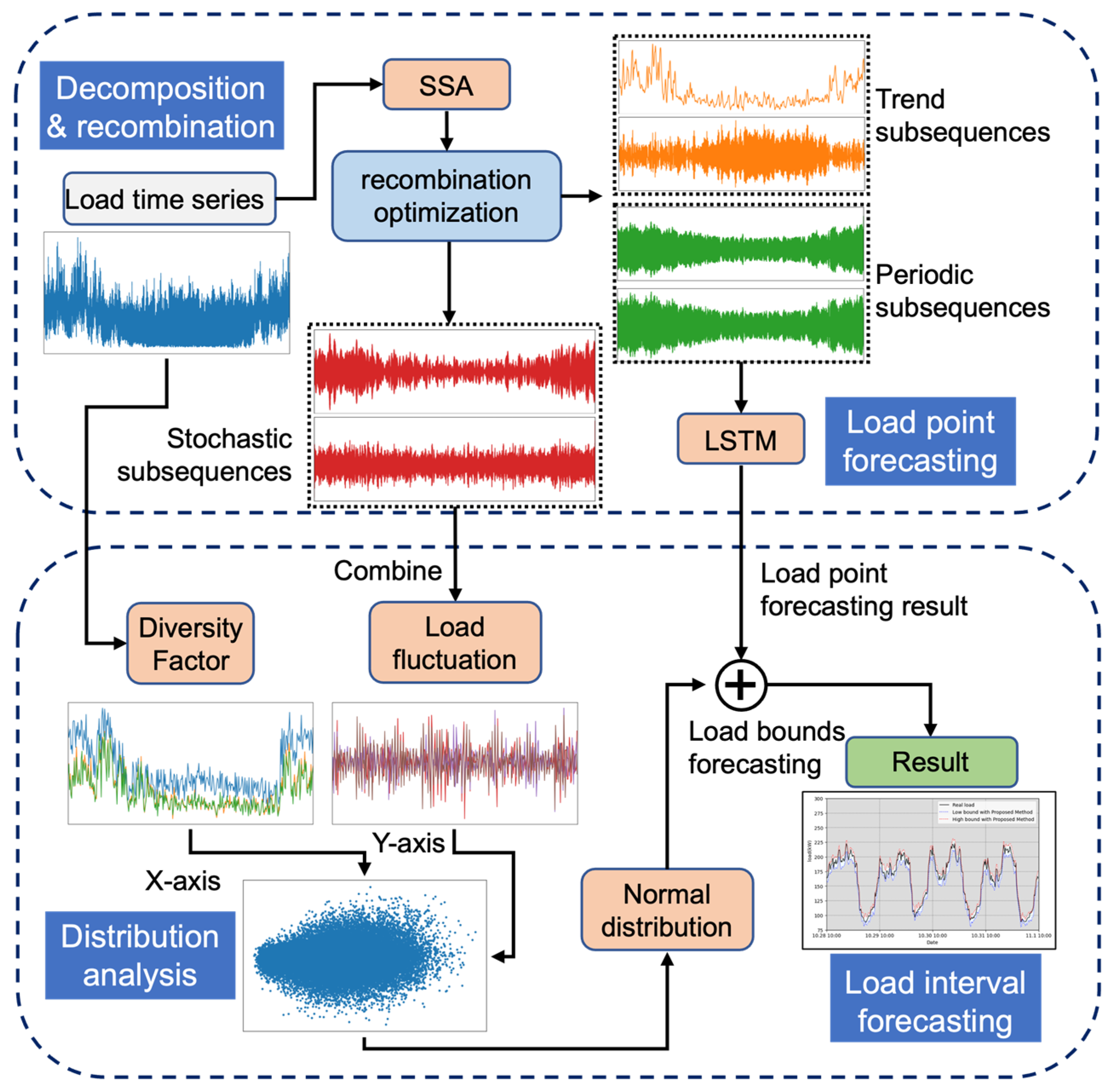
The short-term load-interval forecasting model proposed in this paper consists of load-point forecasting and load boundaries forecasting. The framework of the model is shown in Figure 4.
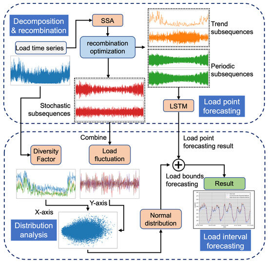
Figure 4.
Framework of the proposed load-interval forecasting method.
In the load-point forecasting process, SSA is used to decompose the load series into different subsequences. Then, the subsequences are recombined into regular subsequences and stochastic subsequences. Finally, the regular subsequence and the temperature data are used for LSTM network training. The load-point forecasting model can be obtained after the training process.
In the load boundaries forecasting process, the stochastic subsequence in the point forecasting process is used as load fluctuation data. DF of the regional residential load is calculated as the indicator of residents’ load consumption consistency. Then, the normal distribution relationship between DF and load fluctuations is analyzed, so the load upper bound and lower bound can be obtained from DF and the 3σ rule in normal distribution. Next, the load daily coincident demand will be forecasted using the same LSTM forecasting model, and the load boundaries will be obtained. Finally, the load boundaries forecasting result and load-point forecasting result are superimposed to obtain the load-interval forecasting result.
3. Case Study
3.1. Example System
In order to verify the performance of the short-term load-interval forecasting with the proposed method, this paper uses the county-wide residential electricity load data of three different counties—Napa in California, Sheridan in Wyoming, and Washington in New York in the United States. All the data come from the National Renewable Energy Laboratory (NREL)’s open-source data [28]. In addition, in the process of constructing the LSTM model, this paper takes 60% of the data as the training set, 20% as the validation set, and the remaining 20% of the data as the test set. For other parts that need to be verified, 80% of the data is used as an experimental set, and the remaining 20% is used as a test set.
All the experimental codes in this paper are based on Python 3.8.13 running under the 20.04.4 Ubuntu release version (Linux kernel v 5.15.0), and the LSTM model is built based on the 1.10.2 version of PyTorch.
3.2. Data Decomposition and Recombination
January’s residential load data in Napa are taken as an example in the orange, green, and red plots in Figure 5. The load data decomposition subsequences processed by SSA can be seen. In other research, the load time series is divided into many subsequences and then recombined to obtain a relatively smooth sequence. The main target of using SSA is to keep the main part of the sequence, obtain the filtered sequences and make the forecasting process much easier. In the proposed method, to divide the load sequence into subsequences with different features, the load sequence is recombined into two different subsequences, the trend subsequence and the stochastic subsequence, and all the subsequences are kept and analyzed separately. The recombination process is described in Section 2.1.3. Since the tendency and the frequency can be seen as the regularities of the load data, the subsequences of noise are recombined into the stochastic subsequence, and the other subsequences are recombined into the regular subsequence.
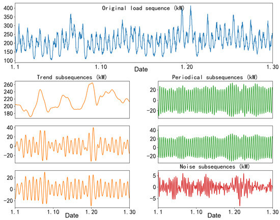
Figure 5.
The subsequences of the load time series processed by SSA.
3.3. Evaluation Metrics
To verify the interval accuracy of the load-interval forecasting model, it is necessary to construct evaluation metrics for the forecasting results. The results of the load forecasting model need to be compared with the actual results to verify the coverage of the model. In order to test the effectiveness of the load-interval forecasting model, this study introduces two indicators, coverage rate (CR) and interval average convergence (IAC), based on the perspectives of forecasting coverage and forecasting model convergence.
Define the frequency at which the actual load value of the coverage rate falls within the load forecasting interval, and set the load forecasting interval of this interval as , the upper and lower intervals as and , and the real load value as . Then it can be considered that the interval forecasting result satisfying is the accurate value. The formula for calculating coverage is as follows:
where n is the number of times the actual load value falls within the forecasting interval in the sample, and m is the total number of samples of the actual load value. Compared to point forecasting results, interval forecasting has the ability to cover the real load data rather than how close the forecasting results are to the actual results. Therefore, the CR reflects the accuracy of the interval forecasting results.
Define the IAC as the average interval length of the forecasting interval of the sample, that is, the average of the absolute value of the difference between the upper and lower boundaries of the overall forecasting interval of the sample:
where m is the total number of samples of actual load value, and t is any time. The IAC reflects the convergence degree of the upper and lower thresholds of the model in the interval forecasting model. Under similar coverage, the smaller the IAC is, the smaller the redundant forecasting value generated by the model, and the better the interval forecasting performance of the model.
3.4. Normal Distribution Analysis of DF and Load Fluctuation
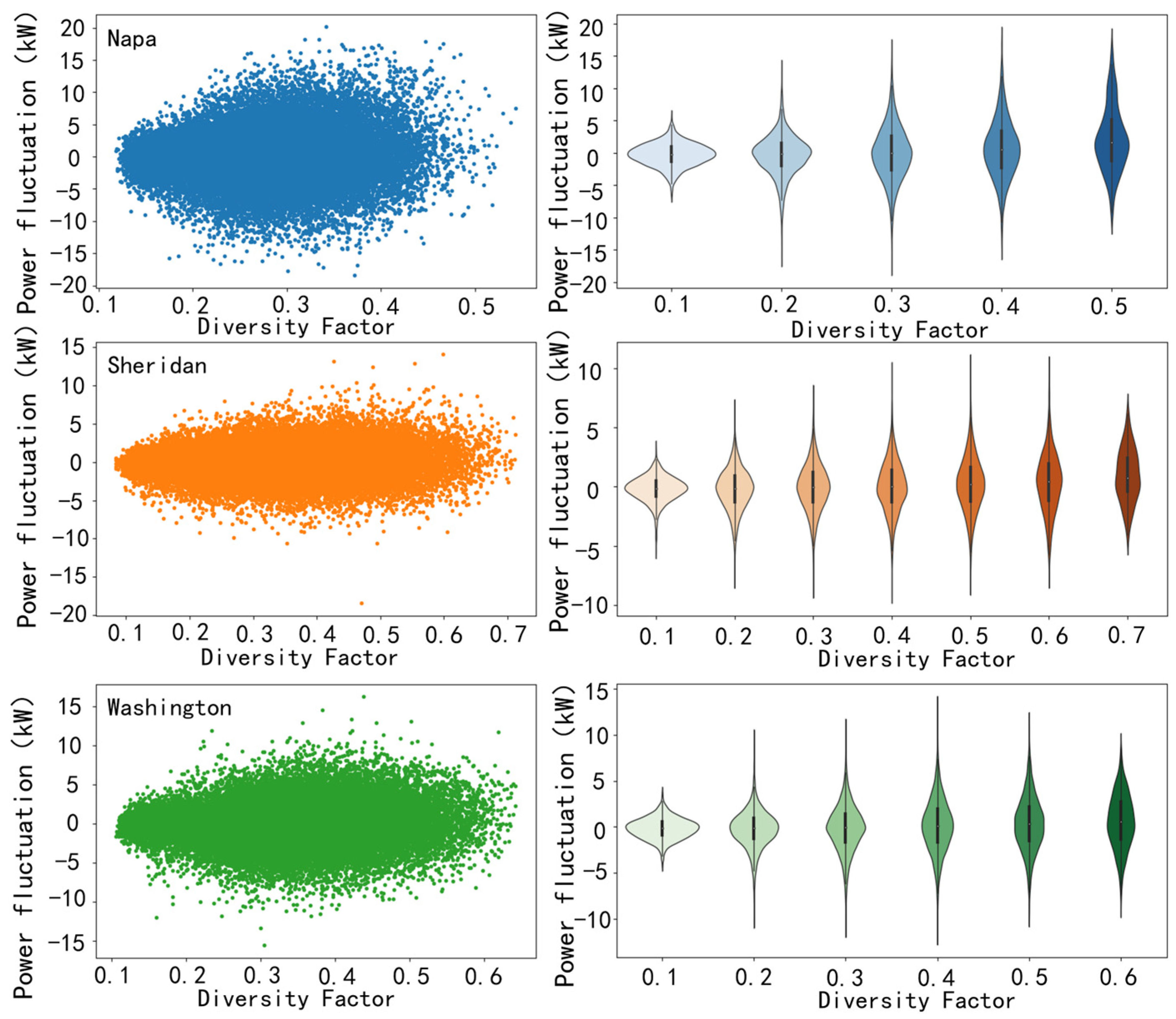
As shown in Figure 6, different scatter distributions illustrate how the stochastic subsequence and DF interact in the three counties. Different DFs are plotted along the x-axis, while the stochastic subsequence’s load fluctuations are plotted along the y-axis. This study creates a violin diagram of the relationship between DF and load fluctuation, taking into account the sample size of the data in the three counties, in order to ensure the rationality of the sample size under different DFs. The violin plots are displayed on the right side of Figure 6 after the outliers are removed. The chart shows that there are some similarities in the relationship between DF and fluctuations in various regions when taking into account the load fluctuations corresponding to DF in different counties. The load fluctuation initially increases and then reduces as DF steadily increases, with the fluctuation data fluctuating around 0 at any given point. As a result, load fluctuations corresponding to various DFs have the same distributional features, and DF and load fluctuation can be conceptualized as a statistical distribution model.

Figure 6.
The relationship between diversity factor and load fluctuation in three counties.
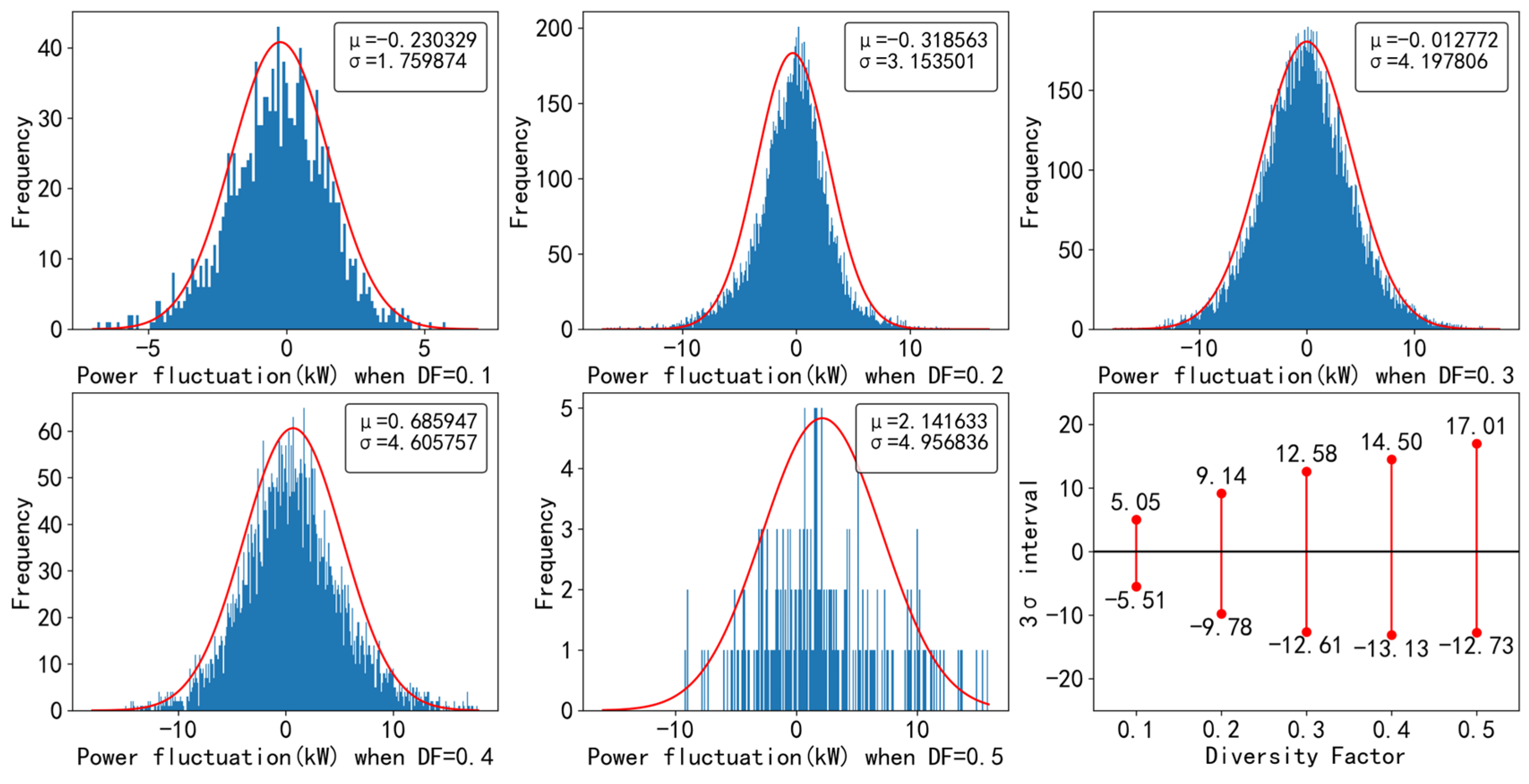
The distribution of each load fluctuation can be better fitted based on statistical analysis. Figure 7 shows the normal distribution of load fluctuations under different DF corresponding data in Napa. There are clear normal distribution characteristics, and the statistical mean of load fluctuations fluctuates around 0. Additionally, the distribution properties in the other two counties are comparable. Table 1 displays the outcomes of the normal distribution study. Therefore, this work quantifies the distribution relationship of load fluctuations under the related DF in the three different counties under analysis based on the normal distribution. DF and the 3σ rules in normal distribution are used to forecast load fluctuations of different counties, that is, when the mean value and standard deviation of the load fluctuation are μ and σ, respectively, the probability of load fluctuations occurring between μ ± 3σ is 99.74%.
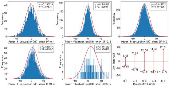
Figure 7.
Normal distribution relationship under different DFs in Napa (The red line shows the outline of the normal distribution).

Table 1.
Normal distribution parameters under different DFs in three counties.
3.5. Load-Interval Forecasting and Results
By adding the load-point forecasting result from the SSA-LSTM and the load boundaries forecasting results from the prior normal distribution, the load-interval forecasting result can be obtained. The load-interval forecasting result in Napa from 28 October to 1 November when the standard deviation is 3σ is presented in Figure 8. The CR and IAC of different σ rate intervals in the three counties are recorded in Table 2. When the entire load-point forecasting coverage is examined, the forecasting accuracy range is generally commensurate with the theoretical range for the real normal distribution.
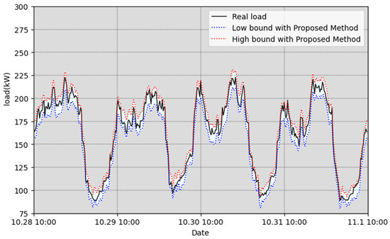
Figure 8.
The forecasting results in Napa (3σ).
Table 2.
Interval forecasting model indicators under different σ magnifications.
4. Discussion
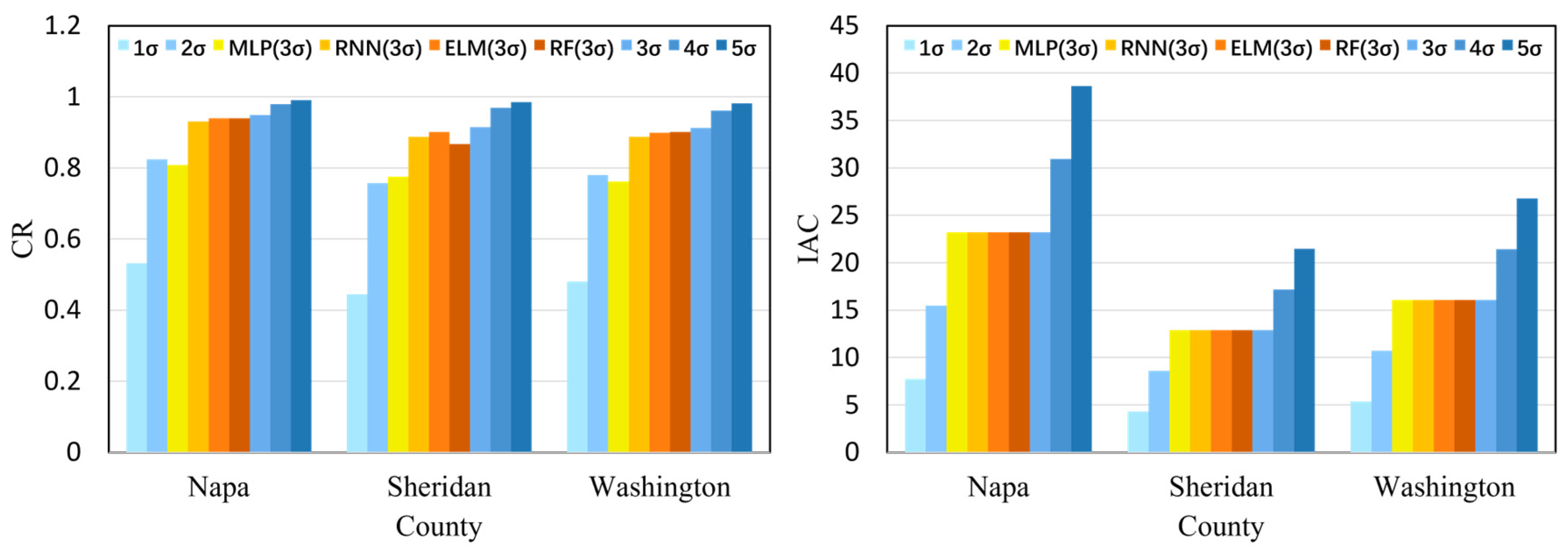
For the load-point forecasting part, this paper builds load-interval forecasting models for three counties using the aforementioned widely used load-interval forecasting methods with different neural networks (MLP and RNN), and the ELM [6] and RF [8] methods, which are introduced in the literature review part and are also added to forecast load points as comparisons. On the other hand, although the load-point forecasting modeling is different from the proposed method, the fluctuation analysis processes of the MLP, RNN, ELM and RF approaches are the same as the proposed method. Then, this paper compares the CR and IAC of various approaches to demonstrate the efficacy and reliability of the proposed method, and the results can be seen in Figure 9.
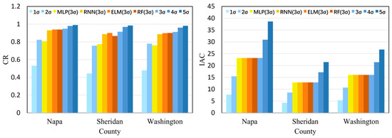
Figure 9.
The CR and IAC comparison of different load-point forecasting methods in three counties.
As for the load-point forecasting methods, when taking the three-times standard deviation, the ELM and RF show similar CRs with the proposed method, but the CRs of the proposed method are (17.50%, 1.95%, 1.05%, 0.97%), (17.95%, 3.02%, 1.49%, 5.49%), (19.79%, 2.79%, 1.43%, 1.18%) higher than MLP/RNN/ELM/RF models in the three counties, respectively. Although the IAC results of these methods are the same due to the same load fluctuation analysis process, the CR results of the proposed methods are lower than the proposed LSTM methods, which have been proven more effective in the load-point forecasting process.
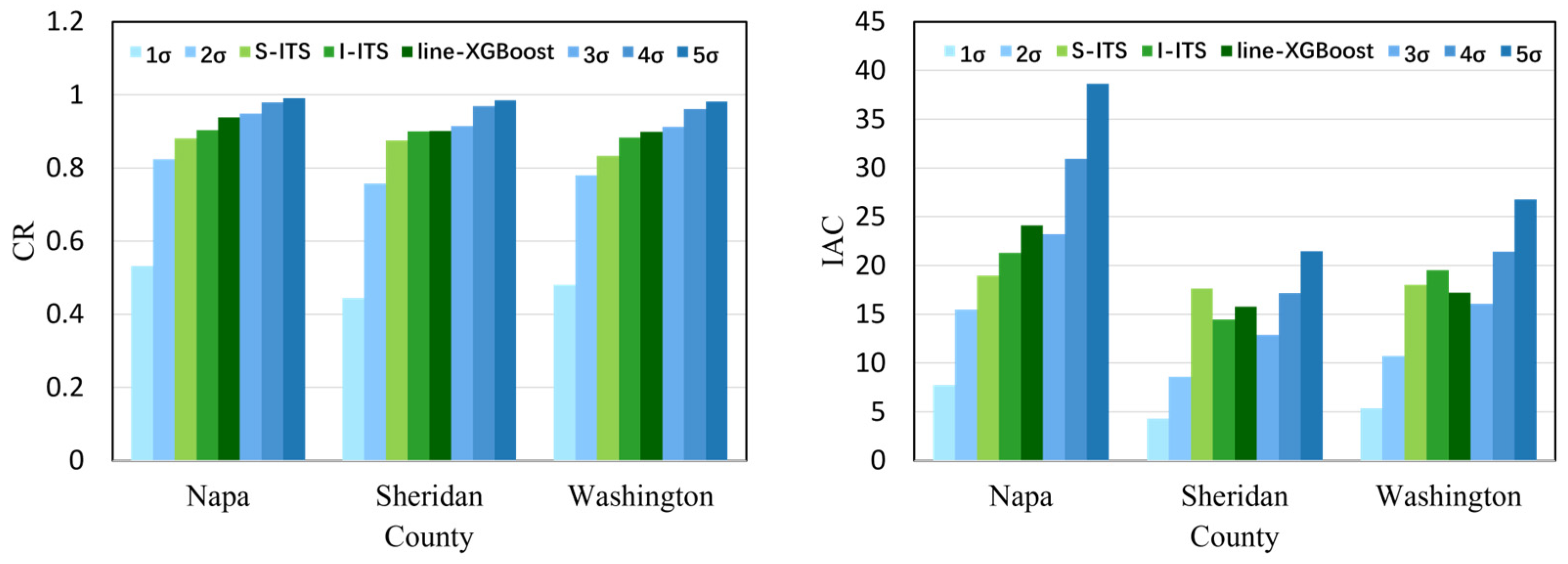
For the load-interval forecasting part, the two methods that use load value to obtain the load-interval forecasting model both obtain the interval time series (ITS) by zooming the coordinate axis, then the methods forecast the upper and lower boundaries of the load independently and synchronously, respectively (called I-ITS and S-ITS) by the same SSA-LSTM process [13]. Besides this, the line-XGBoost regression [19] method is also applied as a comparison, which applies XGBoost on load fluctuation analysis. The indicators’ comparison results are shown in Figure 10. Given that the proposed method does not group the original data, obviously, it has a better level of time granularity than the ITS methods. When taking the three-times standard deviation, the CRs of the proposed method are (7.80%, 5.03%, 1.11%), (4.55%, 1.66%, 1.49%), (9.52%, 3.37%, 1.42%) higher than S-ITS/I-ITS/line-XGBoost methods in three counties, respectively.

Figure 10.
The CR and IAC comparison of different load-interval forecasting methods in three counties.
In addition, according to Figure 10, the I-ITS and S-ITS methods are more stable than the 2σ interval of the proposed method on the CR, but when taking three-times the standard deviation, the proposed method shows advantages in CRs. For IACs, the IACs of the proposed method are (−18.19%, −8.15%, 3.97%), (36.97%, 21.92%, 22.59%), (12.31%, 21.59%, 7.22%) compared to I-ITS/S-ITS/line-XGBoost methods in the three counties, respectively. Since IAC shows the degree of convergence of the results, a low IAC shows a better performance. We can see that although the IACs are better in Sheridan and Washington with our proposed method, the result in Napa is worse when compared to ITS methods. To clarify this issue, we further analyzed the original data and compared the electricity consumption and temperature data of Napa with the other counties. The county Napa is in California, where the climate is warm/hot all year round, while the other two counties are in areas with distinct four seasons. Since temperature change leads to differences in the choice of electrical appliances, the electricity consumption features of residents in Napa will show lower inconsistencies. In other words, the standard deviation (σ) in Napa is bigger than that in the other two counties, and this is because the temperature in Napa is warm and stable, which leads to relatively unobvious differences in electricity consumption behavior. Thus, the IAC of I-ITS and S-ITS methods are only better than the 2σ interval in Napa, but in the other two counties, the IAC of the ITS methods is close to the 4σ/5σ standard deviation, in other words, the average degree of redundancy forecasted by them is higher. Furthermore, the proposed method completely explains the intervals in the forecasting results, that is, the normal distribution of residents’ electricity consumption behaviors, so the interpretability of the interval forecasting results is better than the ITS methods. To sum up, the method proposed in this paper has better performance than the ITS methods and the load fluctuation analysis with other neural networks. In conclusion, the proposed method shows better overall performance and applicability.
5. Conclusions
Load-interval forecasting plays an important role during the transformation of power systems. This paper proposes a load-interval forecasting model that takes into account the regularity and stochasticity of the energy consumption features of the regional residential load simultaneously. In general, this method includes three steps: load-point forecasting based on SSA-LSTM, residents’ behavior-load uncertainty analysis based on DF-load fluctuation normal distribution, and load-interval forecasting. The characteristics of the proposed method can be concluded as follows:
- This research suggests a load-interval forecasting method based on nonlinear fitting and statistical analysis that takes into account both the regular feature and the stochastic feature in the load time series. The LSTM deep learning network combines and forecasts the load trend and periodic information, and the normal distribution displays the load stochastic features.
- SSA is used to decompose the load sequence, and RMSE calculation is employed to carry out the recombination process, resulting in subsequences with regular and stochastic properties. In order to fully utilize the original load data, the regular subsequence is used to train the LSTM load-point forecasting model, and the stochastic subsequence is used to conduct the load fluctuation analysis.
- Statistical analysis and the normal distribution are used to create the mapping from the diversity factor to the load fluctuation, which relates the load stochastic feature and the consistency of the residents’ load consumption. Since the forecasted load boundaries are based on a probability model, well-established normal distribution rules improve interval forecasting performance.
It should be mentioned that although this research introduces a novel approach for load-interval forecasting, the load-point forecasting part in the proposed approach has a very strong research foundation. Related methods are continually revised, and new load-affecting components are presently being identified or researched. Therefore, the load-point forecasting results may be further optimized if new approaches, procedures, or tools suggested or researched by other researchers are employed, and as a result, the load-interval forecasting results will also be improved. In addition, the DF in this study is constrained by the sample size to the rounded result of one decimal place (otherwise, the sample size of the different DFs will be too small to reach a meaningful conclusion). If there were a larger sample in the future, the value of the DF could become more refined. Furthermore, the DF is only a method to quantify the consistency of household electricity consumption, and many researchers have conducted in-depth studies on the characteristics of household electricity consumption behavior. Factors like the weather, the seasons, and holidays will also have an impact on household power demand [29,30]. By employing the novel technique for quantifying the characteristics of household energy consumption, new research perspectives might be obtained, and the characteristics of load variations and household users could be further optimized as well. On the other hand, the normal distribution is one of the distribution models which may not be able to fully describe the features of the load consumption behavior. Therefore, further research can be specialized on the distribution research to find the most fitted statistical distribution model for the residents’ load consumption consistency/users’ behavior relationship. Lastly, in places where the climate is stable all year round, the load fluctuation forecasting results tend to be higher. To solve this problem, it is worth mentioning that residents’ behavior is so complex that the load consumption behavior only constitutes a small part, thus, although the model performs better than other methods, if other behaviors like the residents’ economic behavior during load consumption can be researched and introduced into load forecasting research in some way, the proposed method could be further optimized.
Author Contributions
Conceptualization, R.Z. and Z.Z.; methodology, R.Z. and M.Y.; software: R.Z. and Y.G.; validation, Y.G. and J.S.; writing—original draft preparation: R.Z. and Z.Z.; writing—review and editing, M.Y., J.S. and X.S.; supervision: Y.S. and Y.W.; project administration: R.Z., Y.S. and Y.W. All authors have read and agreed to the published version of the manuscript.
Funding
This paper is supported by the State Grid JiangSu Electric Power Co. LTD, State Grid Co., Ltd. Science and Technology Project through Grant No. 5100-202118566A-0-5-SF.
Data Availability Statement
The data related to the resident in the U.S. presented in this study are openly available in [End-Use Load Profiles for the U.S. Building Stoc] at [https://doi.org/10.25984/1876417], reference number [28]. The load forecasting analysis and results related data presented in this study are available on request from the corresponding author. The data are not publicly available due to the researchers’ need to apply for relevant intellectual property and write new articles.
Conflicts of Interest
Author Jie Song is employed by the company Nari Group Corporation State Grid Electric Power Research Institute, and author Xuanxuan Shi is employed by the company State Grid Nanjing Power Supply Company. The remaining authors declare no conflict of interest. The funders had no role in the design of the study; in the collection, analyses, or interpretation of data; in the writing of the manuscript; or in the decision to publish the results.
References
- Yang, Q.; Wang, H.; Wang, T.; Zhang, S.; Wu, X.; Wang, H. Blockchain-based decentralized energy management platform for residential distributed energy resources in a virtual power plant. Appl. Energy 2021, 294, 117026. [Google Scholar] [CrossRef]
- Jordehi, A.R. A stochastic model for participation of virtual power plants in futures markets, pool markets and contracts with withdrawal penalty. J. Energy Storage 2022, 50, 104334. [Google Scholar] [CrossRef]
- Imani, M. Electrical load-temperature CNN for residential load forecasting. Energy 2021, 227, 120480. [Google Scholar] [CrossRef]
- Estebsari, A.; Rajabi, R. Single residential load forecasting using deep learning and image encoding techniques. Electronics 2020, 9, 68. [Google Scholar] [CrossRef]
- Eskandari, H.; Imani, M.; Moghaddam, M.P. Convolutional and recurrent neural network based model for short-term load forecasting. Electr. Power Syst. Res. 2021, 195, 107173. [Google Scholar] [CrossRef]
- Liu, C.; Sun, B.; Zhang, C.; Li, F. A hybrid prediction model for residential electricity consumption using holt-winters and extreme learning machine. Appl. Energy 2020, 275, 115383. [Google Scholar] [CrossRef]
- Oreshkin, B.N.; Dudek, G.; Pełka, P.; Turkina, E. N-BEATS neural network for mid-term electricity load forecasting. Appl. Energy 2021, 293, 116918. [Google Scholar] [CrossRef]
- Fan, G.-F.; Zhang, L.-Z.; Yu, M.; Hong, W.-C.; Dong, S.-Q. Applications of random forest in multivariable response surface for short-term load forecasting. Int. J. Electr. Power Energy Syst. 2022, 139, 108073. [Google Scholar] [CrossRef]
- Hong, Y.; Zhou, Y.; Li, Q.; Xu, W.; Zheng, X. A deep learning method for short-term residential load forecasting in smart grid. IEEE Access 2020, 8, 55785–55797. [Google Scholar] [CrossRef]
- Rafi, S.H.; Masood, N.A.; Deeba, S.R.; Hossain, E. A short-term load forecasting method using integrated CNN and LSTM network. IEEE Access 2021, 9, 32436–32448. [Google Scholar] [CrossRef]
- Wang, Y.; Zhang, N.; Chen, X. A short-term residential load forecasting model based on LSTM recurrent neural network considering weather features. Energies 2021, 14, 2737. [Google Scholar] [CrossRef]
- Liu, B.; Huang, Q.; Zhao, J.; Hu, W. A computational attractive interval power flow approach with correlated uncertain power injections. IEEE Trans. Power Syst. 2019, 35, 825–828. [Google Scholar] [CrossRef]
- Yang, D.; Guo, J.-E.; Sun, S.; Han, J.; Wang, S. An interval decomposition-ensemble approach with data-characteristic-driven reconstruction for short-term load forecasting. Appl. Energy 2022, 306, 117992. [Google Scholar] [CrossRef]
- Sanjari, M.J.; Karami, H. Optimal control strategy of battery-integrated energy system considering load demand uncertainty. Energy 2020, 210, 118525. [Google Scholar] [CrossRef]
- Judge, M.A.; Manzoor, A.; Maple, C.; Rodrigues, J.J.; Islam, S.U. Price-based demand response for household load management with interval uncertainty. Energy Rep. 2021, 7, 8493–8504. [Google Scholar] [CrossRef]
- Teshnehdel, S.; Mirnezami, S.; Saber, A.; Pourzangbar, A.; Olabi, A.G. Data-driven and numerical approaches to predict thermal comfort in traditional courtyards. Sustain. Energy Technol. Assess. 2020, 37, 100569. [Google Scholar] [CrossRef]
- Pearre, N.S.; Swan, L.G. Statistical approach for improved wind speed forecasting for wind power production. Sustain. Energy Technol. Assess 2018, 27, 180–191. [Google Scholar] [CrossRef]
- Anvari, M.; Proedrou, E.; Schäfer, B.; Beck, C.; Kantz, H.; Timme, M. Data-driven load profiles and the dynamics of residential electricity consumption. Nat. Commun. 2022, 13, 4593. [Google Scholar] [CrossRef]
- Wang, Y.; Sun, S.; Chen, X.; Zeng, X.; Kong, Y.; Chen, J.; Guo, Y.; Wang, T. Short-term load forecasting of industrial customers based on SVMD and XGBoost. Int. J. Electr. Power Energy Syst. 2021, 129, 106830. [Google Scholar] [CrossRef]
- Zhu, J.; Dong, H.; Zheng, W.; Li, S.; Huang, Y.; Xi, L. Review and prospect of data-driven techniques for load forecasting in integrated energy systems. Appl. Energy 2022, 321, 119269. [Google Scholar] [CrossRef]
- Serrano-Guerrero, X.; Briceño-León, M.; Clairand, J.-M.; Escrivá-Escrivá, G. A new interval prediction methodology for short-term electric load forecasting based on pattern recognition. Appl. Energy 2021, 297, 117173. [Google Scholar] [CrossRef]
- Haben, S.; Arora, S.; Giasemidis, G.; Voss, M.; Greetham, D.V. Review of low voltage load forecasting: Methods, applications, and recommendations. Appl. Energy 2021, 304, 117798. [Google Scholar] [CrossRef]
- Colebrook, J.M. Continuous plankton records-zooplankton and environment, northeast Atlantic and North-Sea, 1948–1975. Oceanol. Acta 1978, 1, 9–23. [Google Scholar]
- Gasparin, A.; Lukovic, S.; Alippi, C. Deep learning for time series forecasting: The electric load case. CAAI Trans. Intell. Technol. 2022, 7, 1–25. [Google Scholar] [CrossRef]
- Hochreiter, S.; Schmidhuber, J. Long short-term memory. Neural Comput. 1997, 9, 1735–1780. [Google Scholar] [CrossRef]
- Kersting, W.H. Distribution System Modeling and Analysis; CRC Press: Boca Raton, FL, USA, 2017. [Google Scholar]
- Sirignano, J.; Spiliopoulos, K. Mean field analysis of neural networks: A central limit theorem. Stoch. Process. Their Appl. 2020, 130, 1820–1852. [Google Scholar] [CrossRef]
- Wilson, E.; Parker, A.; Fontanini, A.; Present, E.; Reyna, J.; Adhikari, R.; Bianchi, C.; CaraDonna, C.; Dahlhausen, M.; Kim, J.; et al. End-Use Load Profiles for the U.S. Building Stock; National Renewable Energy Laboratory: Golden, CO, USA, 2021. [Google Scholar] [CrossRef]
- Hammad, M.A.; Jereb, B.; Rosi, B.; Dragan, D. Methods and models for electric load forecasting: A comprehensive review. Logist. Sustain. Transp. 2020, 11, 51–76. [Google Scholar] [CrossRef]
- Shen, M.; Lu, Y.; Wei, K.H.; Cui, Q. Prediction of household electricity consumption and effectiveness of concerted intervention strategies based on occupant behaviour and personality traits. Renew. Sustain. Energy Rev. 2020, 127, 109839. [Google Scholar] [CrossRef]


Disclaimer/Publisher’s Note: The statements, opinions and data contained in all publications are solely those of the individual author(s) and contributor(s) and not of MDPI and/or the editor(s). MDPI and/or the editor(s) disclaim responsibility for any injury to people or property resulting from any ideas, methods, instructions or products referred to in the content. |
© 2023 by the authors. Licensee MDPI, Basel, Switzerland. This article is an open access article distributed under the terms and conditions of the Creative Commons Attribution (CC BY) license (https://creativecommons.org/licenses/by/4.0/).