Article

Optimization of Air Handler Controllers for Comfort Level in Smart Buildings Using Nature Inspired Algorithm

1
Department of Electrical Technology Section, Universiti Kuala Lumpur British Malaysian Institute (UniKL BMI), Kuala Lumpur 53100, Malaysia
2
Department of Electrical Engineering Section, Universiti Kuala Lumpur British Malaysian Institute (UniKL BMI), Kuala Lumpur 53100, Malaysia
3
Department of Electrical Engineering, Universiti Teknologi MARA (UiTM), Shah Alam 40450, Malaysia
*
Author to whom correspondence should be addressed.
Energies 2023, 16(24), 8064; https://doi.org/10.3390/en16248064
Submission received: 2 February 2023 / Revised: 25 June 2023 / Accepted: 28 July 2023 / Published: 14 December 2023

Abstract

:
This research seeks to improve the temperature control of AHU in building sub-levels using optimization algorithms. Specifically, the study applies the FA and PSO algorithms to optimize the PID control of AHU’s temperature. The study addresses the issue of temperature control in building sub-levels, which is a common challenge in HVAC systems. The study uses optimization algorithms and a nonlinear model to improve temperature control and reduce fluctuations in temperature from the desired setting. Additionally, a NL-ARX algorithm is utilized to create a nonlinear model based on the thermal dynamics and energy behavioral patterns of ACMV cooling systems. The study evaluates the performance of three controllers—PID, FA-PID, and PSO-PID—based on ITSE as a performance index. The study compares the performance of these controllers to achieve the desired temperature setting, and it analyses the influence of temperature regulation on occupant comfort levels. In this study, we compare different controllers using ITSE as a performance indicator. This shows how well different optimization algorithms work at setting the right temperature. The research gap is the lack of efficient temperature control solutions in building sub-levels that can optimize occupant comfort and energy efficiency. The experimental findings confirm that PSO-PID outperforms conventional PID and FA-PID optimization in terms of achieving the goal objective via computational complexity. Overall, this study’s focus is to explore and compare different optimization algorithms to improve temperature control and occupant comfort in building sub-levels.

1. Introduction

An ACMV system is a cooling system which is used globally in many tropical countries as a cooling mechanism [1]. ACMV systems are designed to maintain a comfortable atmosphere in an air-conditioned space regardless of the outside ambient temperature and humidity conditions. Chilled water systems for central air-conditioning are frequently chosen to be installed in commercial buildings and industries due to their capability to handle a significant amount of cooling demand. The primary components of a central air-conditioning system are cooling towers, chilled water pumps (CHWPs), CDWP, chillers, and AHU [2]. The operating conditions of ACMV systems directly influence energy efficiency and internal climate; hence, the research would have a substantial influence on energy conservation, lowering pollution from greenhouse gases of carbon dioxide, and the development of a healthier indoor environment.
According to the Statistical Review of World Energy 2021 report, energy consumption utilizing non-renewable resources including fossil fuels use has decreased almost three-quarters of the net decline. Alternative renewable sources of energy such as hydro, nuclear, and wind increased by 10.7 percent, while solar electricity increased by a record 20 percent of current energy consumption. According to real-time data, oil will be depleted in 40–50 years, while natural gas and coal will be depleted in 160 and 410 years, respectively [3]. The issue of decreasing energy resources has received growing attention around the world.
Hence, to optimize energy usage, the concept of energy efficiency has been applied in a variety of fields, including buildings, transportation, manufacturing, and industry. In Malaysia, the building industry consumes the greatest amount of energy at 40 percent when compared to the industry sector at 32 percent and the transportation sector at 28 percent [4]. One of the primary contemporary problems is the ever-increasing quantity of structures in urban centers. The research is mostly concerned with the energy conservation of smart buildings. As per energy assessments for buildings, ACMV systems are among the most energy-intensive components [5]. Traditional office buildings in Malaysia often utilize well over 50 percent of their entire electricity consumption to energize air conditioning due to the hot and humid tropical weather conditions [6].
As shown in Figure 1, office building electricity distribution is divided into four categories: air-conditioning load, lighting, office equipment, and others. Building occupants’ productivity and health can be negatively impacted by indoor environmental conditions controlled by ACMV systems [7,8]. Particularly in tropical nations such as Malaysia, ACMV systems are crucial for keeping a suitable indoor climate [9]. These systems demand a great deal of energy, though, so increasing their effectiveness is essential to conserve energy and preserve health. The study’s objective was to enhance the temperature management and equilibrium of ACMV systems to increase their efficiency. The study constructed a simulation model using actual data from smart buildings as a suggestion to provide more efficient temperature control systems.
The model’s PID controller has been tweaked to deliver the desired optimal output. The analysis showed that the building’s inside temperature could not be stabilized to its full potential by the current ACMV operation. Therefore, the study is necessary to enhance the ACMV system’s control and increase its stability. The algorithm for the study is created using the specified temperature setting demanded by building occupants. Recent studies on how to provide thermal comfort without using a lot of energy have mostly concentrated on methods to control temperature control systems such as HVAC and ACMV. It is feasible to improve control, maintain a comfortable indoor atmosphere, and conserve energy by implementing optimization approaches in control simulations.
The paper’s structure begins with an introductory part containing a summary of the research topics and emphasizing the primary issues that the study seeks to answer. The second portion is background research on the ACMV-related algorithm and thermal comfort, which includes a full literature review on the ACMV system, and the methods utilized in it. It is further subdivided into three sections: thermal comfort, air conditioning, and the ACMV system.
Thirdly, the ACMV modelling and NL-ARX subsection describe the methods employed in the study. It is further subdivided into five sections, which are as follows:
  • Optimization of air handler controllers;
  • ACMV system modeling with thermal comfort, which illustrates how the NL-ARX method was used to create a nonlinear model based on the ACMV system’s thermal dynamics and energy behavioral patterns;
  • Positioning of Temperature Sensors;
  • Simulation Model;
  • Optimization of ACMV Control System: This subsection describes how the FA and PSO methods were used to optimize the ACMV control system.
Fourthly, the study’s findings are presented in the Section 4, which also elaborates on them. The performance of the optimization techniques employed in the study is also compared, and the Section 5 concludes by summarizing the results and contributions of the study. It also examines the study’s limitations and offers ideas for future research trajectories.

2. ACMV Related Algorithm and Thermal Comfort

Many research investigations have been conducted to increase a building’s energy efficiency, considering various geographic areas and their cooling and heating requirements. [10]. Efficiency in using electricity for heating is prioritized in locales with long or short winters, whereas energy usage for cooling is preferred in low-latitude regions with hot, humid summers. [11,12]. Thermal comfort can be divided into two categories: passive and active. The passive type considers aspects connected to the surrounding environmental conditions, while the active type relies on occupant physiological parameters. [13].
The ACMV system, which comprises the cooling tower, chiller, CHWP, AHU, and CDWP, is the most widely used cooling method in tropical areas [14]. Data gathered using modelling techniques is analyzed to translate the process for regulating the inside ambient temperatures into mathematical algorithms, which is one of the many ways that researchers are constantly trying to increase the performance of the cooling system at a cheaper cost compared to directly installing a new control system and testing it on site. In general, this field of study seeks to increase energy effectiveness while preserving thermal comfort for building occupants.
Consequently, to model a building’s room temperature, several algorithms are studied to determine their suitability for determining the temperature conditions in the building, which are influenced by a variety of factors such as outdoor temperature, current temperature, and updated temperature. There are two types of algorithms considered: linear variable frameworks such as the ARX and ARMAX systems and nonlinear models such as neural network-based NL-ARX [15]. Linear and nonlinear algorithms are discussed in detail in the section on indoor temperature modelling techniques.
Following the successful creation of a model that can translate the process of controlling the building’s indoor temperature using an ACMV system while considering all other factors that can influence temperature fluctuations in the building, the research continued in search of the best method for optimizing the ACMV control system’s performance using the optimization method. The firefly algorithm, the genetic algorithm, and particle swarm optimization are examples of algorithms that are inspired by nature.

2.1. Optimization Algorithms

A common strategy in engineering systems for applications is simulation optimization, which uses computer software to forecast the effects of proposed system improvements. A system can be examined more thoroughly in less time and at a cheaper cost with this method. Modelling, computing, and methods of searching are used in optimization procedures, which typically aim to maximize output and reduce operating expenses. Weighting factors were assigned to each cost function when optimizing multiple cost functions [16].
PSO, GA, DE, SA, TS, ACO, BCO, FA, and GSA are the nine classes into which the metaheuristic methods are categorized [17,18]. The PSO and FA are employed in this study to optimize the control settings for the AHU to obtain the ideal temperature and level of comfort in the smart building.
The ambient temperature, adequate lighting, and pure air are three important components of comfort in buildings. An optimization method called the FA was developed due to the way that fireflies flash. Fireflies are solutions that are generated at random, and their brightness depends on how well they perform in terms of the objective function. The FA excels at addressing highly nonlinear, multi-mode optimization issues and is effective due to its quick convergence. Classification, grouping, isolated, continuous, and combinatorial optimization are all possible with the Firefly algorithm [19].
PSO is another optimization technique that draws inspiration from the biological swarm motions of fish and bird schooling. PSO has been employed in almost every field of optimization; however, it has some limitations, including early convergence and getting stuck in local optima. PSO techniques can occasionally be outperformed by other strategies, such as firefly algorithms and cuckoo detection algorithms [20].
The basis for GA is biological evolution, which includes elements such as mutations, crossover, selection, and recombination. These operators are essential to GA since they enable it to mimic real biological processes. A limited and unconstrained optimization problem-solving approach called GA is based on a natural selection process that parallels biological evolution.
The MIGA and MOGA approaches were derived from GA, and MIGA is used to reduce the discrepancy between the real environment and the parameters provided by the user by enhancing the fuzzy logic input. In smart buildings, MOGA is employed to balance thermal comfort and energy consumption depending on two main factors: the air velocity and the outside temperature [21].
In conclusion, simulation optimization, which incorporates modelling, computing, and search approaches, is a crucial method for improving engineering application systems. The Fireflies Algorithm and Genetic Algorithm are two optimization methods with varying biological foundations, strengths, and shortcomings. Another popular optimization method is particle swarm optimization, but it has some limitations. Utilizing these optimization strategies, systems are made more effective, efficient, and comfortable while minimizing costs and maximizing output. Table 1 lists the many optimization techniques applied to energy research.

2.2. Thermal Comfort
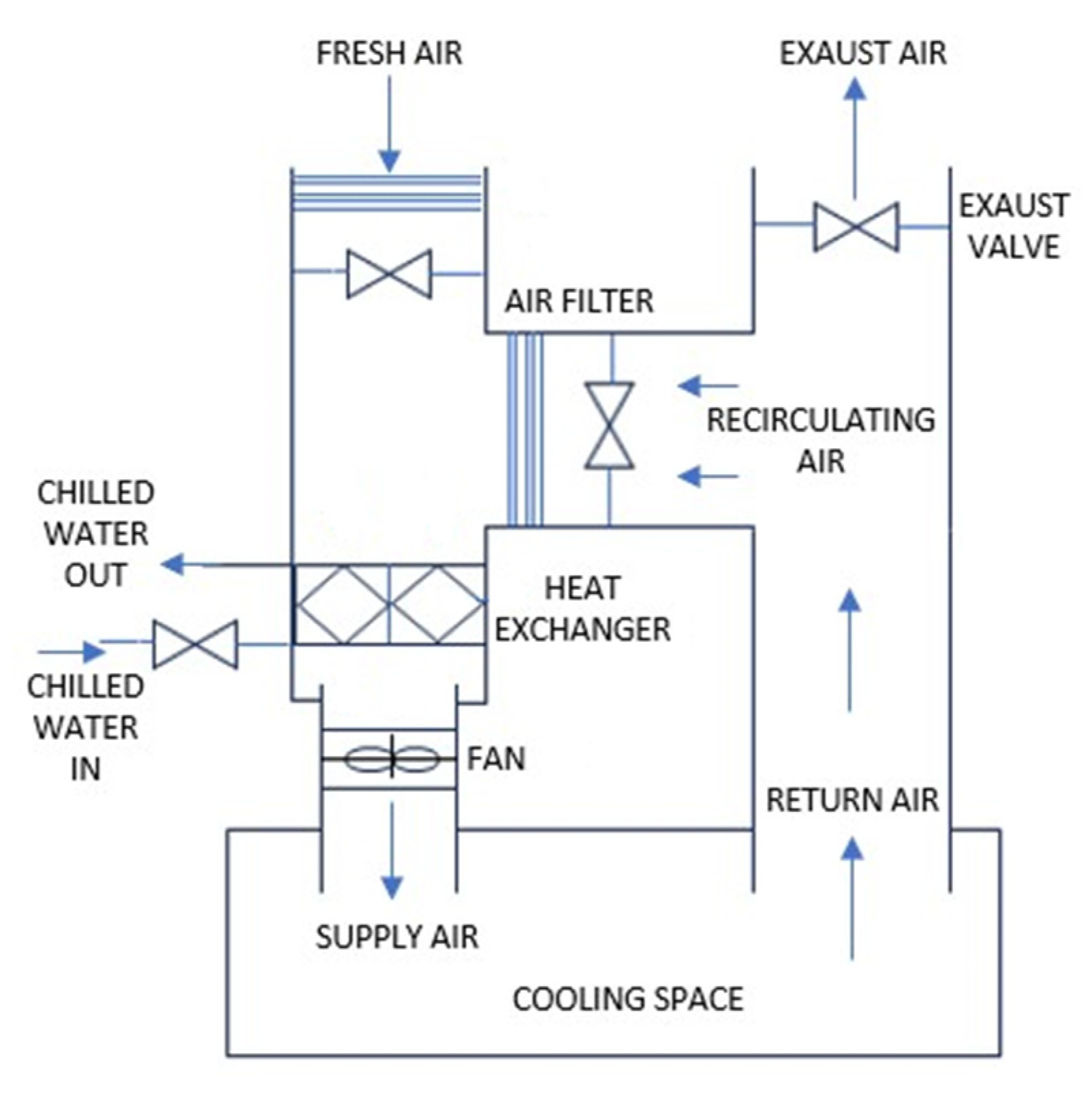
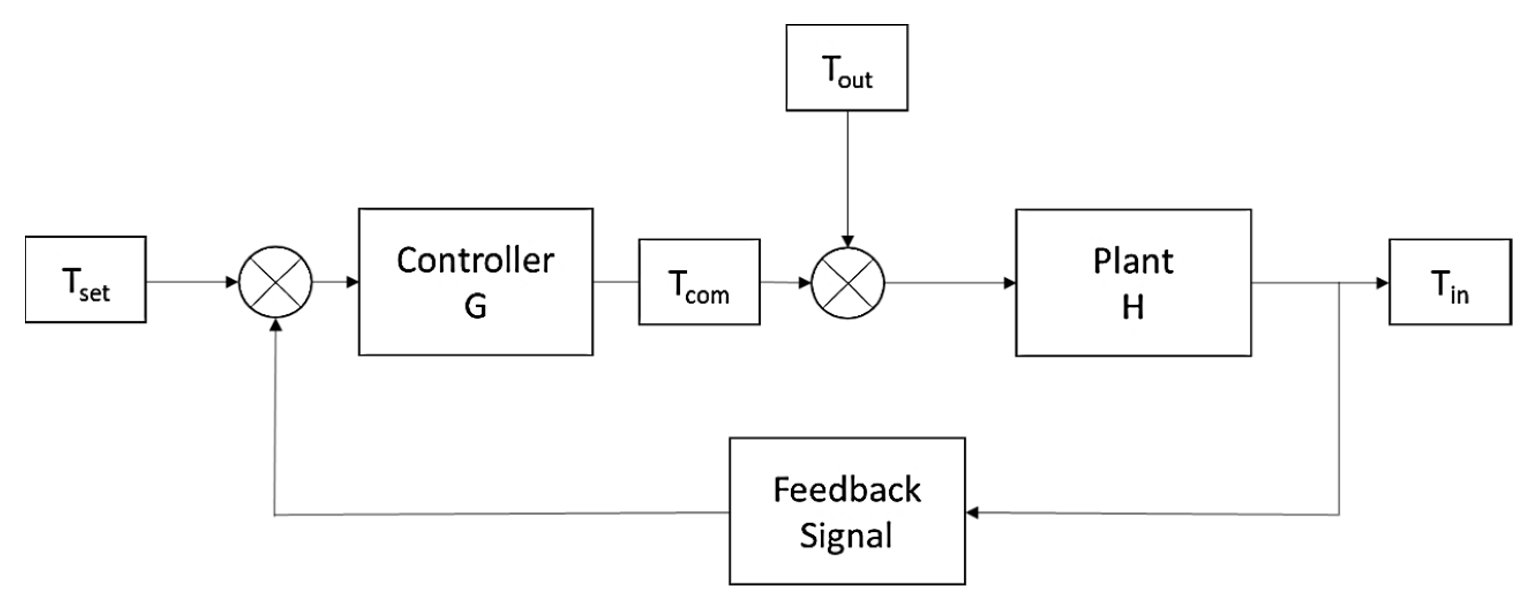
The provision of a comfortable atmosphere is one of the most significant duties of a structure, so that it does not impair the health or performance of those who live or work within it. “Thermal comfort” is described as “the psychological state that conveys happiness with the thermal sensation” by the ISO 7730 standard [35]. Several environmental and physiological aspects must be addressed to fully define the thermal comfort conditions in a location [36]. Temperature, air flow rate, pressure, humidity, sun radiation, velocity, light, noise, and air quality are all environmental elements to consider. The occupant’s state is important physiologically and can influence their thermal comfort and satisfaction. These factors include the occupants’ level of activity, their clothing status, and their gender [37].
One must first understand the target criteria for the relevant thermal ambient characteristics, as well as the methodologies for predicting or measuring them to evaluate thermal comfort. From this underlying principle, it is critical to identify the critical indoor thermal climatic characteristics, quantify their influence on occupants, and determine the impact of buildings and cooling systems on these variables. Thermal comfort studies can be conducted using two distinct methodological approaches: climate chamber testing, also referred to as engineering or passive approaches, and field testing, also referred to as architect or active approaches [38].
The utilization of objective environmental variables allows for a passive approach to evaluating thermal comfort experiences. Three modes of environmental circumstances are occupant objective conditions, radiation, and airfield. Various characteristics, including air temperature, air flow rate, air velocity, air pressure, air quality, and air relative humidity, must be considered while determining airfield conditions [39]. The irradiation levels are mostly driven by the solar radiation during the day. As a result, objective occupant characteristics such as metabolic rate, activity level, and clothing factor must also be considered. The passive technique, including the stochastic stimulus-response idea that supports it, is best suited to situations where thermal comfort is entrusted to the building’s indoor atmospheric system architecture [40].
Occupants are regarded as passive recipients of the thermal stimulation offered by their surroundings, as well as being subjectively appraised with respect to highly particular expectations of what such an environment should appear and be like. Experiences that deviate from anticipation are evaluated unfavorably, and the bigger the disparity between the two, the higher the percentage of discontent.
Fanger developed the most famous and widely adopted approach to measuring thermal comfort [41,42]. By using a set of physical laws and a significant number of inhabitant questionnaires, he introduced the new PMV and PPD models for forecasting occupants’ thermal comfort experiences [43]. Two requirements must be satisfied, according to the findings, for occupants to be thermally comfortable. The first criterion is thermal balance, which is defined by the temperature differential between the skin and the center of the body. The second criterion is a body’s thermal neutrality, which indicates that the heat created by metabolic activities in the organ matches the heat released from the body [44,45].
The PMV model is developed in the following manner, according to ISO-7730:2005:
P M V =   0.303 · e 0.36 M + 0.028     · (   M W Q   )
Q = Q d i f f + Q e v a p + Q r e s p ,
Q d i f f = 3.05 × 10 3 · 5733 6.99 · M W P a 1 / I _ c l   [ T c l 35.7 + 0.028 · ( M W ) ] ,
Q e v a p = 0.42 ·   M W 58.15 ,
Q r e s p = 1.71 × 10 5 · M · 5869 P a + 0.0014 · M · 34 T a ,
T c l = 35.7 0.028 · M W { I c l   3.96 × 10 8 · f c l ·   T c l + 273 4 T m r + 273 4 + f c l   ·   h c · T c l T a } ,
h c = m a x   2.38   ·   T c l T a 1 / 4 12.1   ·   V a  
f c l = 1.00 + 1.29   ·   I c l ,                       I c l 0.078   m 2   K / W 1.05 + 0.645   ·   I c l ,                   I c l > 0.078   m 2   K / W
P a = 6.11   ·   R H 100   ·   10 7.5   ·   T a 237.7 + T a
P P D = 100 95 · e x p 0.03353 · P M V 4 0.2179 · P M V 2
In Equation (2) of the PMV model, Q d i f f is the occupant’s temperature deficiency via diffusion, while Q e v a p and Q r e s p are the occupant’s heat losses via evaporation and respiration, respectively. The PPD model and the PMV model have a significant link, as shown in Equation (10). Accordingly, to obtain optimal results, the PMV and PPD models must be adjusted due to the variety of persons and ambient factors.

2.3. ACMV System

In Malaysia, to ensure thermal comfort within buildings in a tropical environment, ACMV systems must be operational year-round. The average commercial building’s ACMV system uses about 58% of the total energy used in the building [46]. The ACMV’s sustainable planning and improvement of the system greatly contribute to a decrease in electricity consumption and expenses. The obstacle for designers and service providers continues to be developing and managing main cooling systems that are competent while providing the desired IAQ.
Many industrial plants, building managers, and experts would like to discover more about energy-efficient design and optimization options for ACMV systems to lower total operational expenses. Depending on the demand for comfort, several sets of cooling systems are routinely employed in commercial properties and factories. Stand-alone package units, central air-conditioning chilled water systems, VRV systems, and water-cooled package units are examples of these systems. Central air-conditioning chilled water systems are frequently selected to accommodate a reasonably high cooling request [46].
The ACMV system installed as a cooling device to achieve stable temperature comfort in the building meets the study’s criteria. The location of this building in the city of Kuala Lumpur is very relevant for the study since many buildings are built here and there is also a high population density. To provide cool air to the MITI building, a system based on chilled water was constructed and placed in the building. The AHU and FCU’s operational schematics are illustrated in Figure 2.
HVAC systems such as the AHU and FCU are often utilized to keep indoor spaces at a comfortable temperature, humidity level, and air quality. Both systems require numerous crucial stages to operate.
The return air duct is used by the AHU to pull in air and filter out dust and other particles. The AHU may combine filtered air with fresh outdoor air, depending on the ventilation needs and the desired IAQ. A heat exchanger and a refrigeration system are then used by the AHU to warm up or chill the air to the required climate. Depending on the intended comfort levels and the indoor humidity levels, the AHU may also add or remove moisture from the air. The conditioned air is then dispersed throughout the building by the AHU using a system of ducts and diffusers [46].
The FCU pulls air from the return air duct and removes any dust or other particles. The FCU then uses a heat exchanger and a refrigeration system to heat or cool the air to the appropriate temperature. Depending on the intended comfort levels and the indoor humidity levels, the FCU may additionally add or remove moisture from the air. The FCU uses a fan and a grille or diffuser to distribute the conditioned air into the room it serves [46].
In conclusion, the way that AHUs and FCUs function is by conditioning the air to the required temperature and humidity level before distributing it to different areas of the structure. The main distinction between the two is that, whereas FCUs are localized systems that service a single room or region, AHUs are centralized systems that serve several rooms or zones. Both systems are essential to keeping an indoor space comfortable [47].

2.4. ACMV Modelling

The ACMV modelling techniques selected for this research belong to the category driven by data (black box, inverse, or empirical) in the statistical model ARX type. Data-driven models are produced by collecting data from real-world implementations and then using mathematical approaches to link the values of the parameters. This kind of modelling is appropriate for enhancing the efficiency of the current ACMV when adequate training data is available. Statistical frameworks are built on the concept of how a sample of a large database may be obtained by using a specific pattern [48]. These models include ARMAX, linear and polynomial time series regression, ARX, and ARIMA [49].
According to recent research, nonlinear models such as NL-ARX outperform linear models such as ARX and ARMAX in forecasting building space temperatures [50,51]. An evaluation of linear and nonlinear models revealed that while linear models can identify the actual systems’ thermal variables, nonlinear models are better at predicting thermal attributes [52]. Several comparative studies were conducted between these two models, primarily involving the climate and moisture ratio forecasting of building space, and the results of the studies were always in favor of the NL-ARX nonlinear model, which proved to be more accurate in predicting than ARX [51]. The linear model’s inaccuracy is mostly due to the diffusion formula’s nonlinearity in managing temperature and relative humidity.
HVAC system energy consumption is non-linear and changes according to current circumstances. Several factors contribute to the dynamic energy consumption of a HAVC system, including an unstable cooling load, inconsistent weather conditions, an uncontrolled increase and decrease in the number of occupants in the building space, and sudden temperature changes due to a change in the day–night environment. Consequently, to obtain outstanding performance of the controller, typical PID settings must be changed, or new controllers must be used. Statistical models have several advantages, including quick computing time, the capability to perform effectively in the presence of time-varying process noise, and the ability to develop models with limited data [53].

2.5. NL-ARX

Linear ARX models can be refined by nonlinear ARX models. Due to their flexibility, flexible nonlinear functions such as wavelets and sigmoid networks may replicate complicated nonlinear behavior [53]. Formula (11), in which u , y , and e stand for input, output, and noise, respectively, defines the nonlinear ARX system as extending the linear ARX framework. Based on this framework, the predicted current output y ( t ) is the weighted sum of the previous output values as well as the present and previous input values. In contrast to the amount of previous insert parameters that were utilized for predicting the current results, which is marked by n b , the number of prior output terms is represented by n a . The regressors’ weighted total indicates a linear pattern in the nonlinear ARX system, which also utilizes a flexible nonlinear mapping function, F [54].
y t + a 1 y t 1 + a 2 y t 2 + + a n a y t n a                      = b _ 1   u ( t ) + b _ 2   u ( t 1 ) + + b _ n b   u ( t n b + 1 ) + e ( t )
y p t = F y t 1 , y t 2 , y t 3 , , u t , u t 1 , u t 2 ,
F accepts as inputs model regressors. The framework of the nonlinear ARX model can be defined using a collection of nonlinear functions. As an example, F can be interpreted as a weighted total of wavelets that affect the extent that the regressors are within their limits. Nonlinear ARX regressors could signify delay system features or more elaborate delay nonlinear input and output parameters formulations. The structure of nonlinear ARX models includes model regressors and an output expression. The output expression consists of preset offsets for the output and linear and nonlinear equations that work on the model’s regressors to create the result. The nonlinear ARX model output y is computed by the computer program in two steps. It determines regressor values in the first stage by applying present and previous data provided along with past output data. In the second stage, an output function component is utilized to correlate the regressors to the framework’s output. The output function component may contain parallel linear and nonlinear components.
Nonlinear ARX models are commonly employed as black-box architectures. The nonlinear function of the nonlinear ARX model is an agile approximation of irregularities, which does not require physical significance for its variables. Either time-series data without inputs or equally sampled time–domain input–output data can be used to estimate nonlinear ARX models. There could be one or more input and output channels in the input. It is impossible to approximate with frequency domain input. The linear regressors of a nonlinear ARX model can be defined using the orders and delays of the model. The sequence and delay are represented via n a , the number of preceding utilized output expressions to anticipate the present output, n b , the amount of previous input elements utilized for estimating the actual output, and n k , the rate at which samples are taken between the input and the output.

3. Air Handler Controller Optimization

Heating capacity is not an essential demand in tropical regions such as Malaysia when compared to cooling capacity. As a result, ACMV systems demand is high. According to statistics, ACMV systems in a building consume more than 40% of the total electricity [55,56]. Energy-saving ACMV production is critical due to the significant demand for ACMV systems, which might speed up the process of global warming. Consequently, it is crucial to design ACMV systems that are energy efficient via appropriate modelling and optimization to make the most use of energy resources.
Since office workers frequently spend most of their time in the building where they work, the ACMV system’s control of the building’s temperature and humidity must have an impact on the residents’ overall satisfaction. The ergonomic interior environment of the structure is a must to ensure the comfort of the occupants. Work system arrangements, facility conditions, and workplace condition management based on systematic design are the variable factors that are considered to study the level of effectiveness of the workplace environment on individuals, and they are summarized in ergonomic terms. ASHRAE 55 and ISO 7730 are international standards that are used as a reference to set an acceptable temperature range as a comfortable temperature for individuals.
The calculation of the PMV and the PPD index are commonly recognized methods for assessing temperature comfort levels. The methods for modelling the ACMV control system and indoor thermal comfort will be based on passive approaches. By adapting the optimization technique, the problem of inefficient temperature regulation to attain the required thermal comfort will be improved, allowing the system to not only reach the target temperature faster but also become more stable.
As shown in Figure 3, the simulation model for the building temperature control system was developed utilizing several factors and is composed of several primary components. The room or system plant block is combined with an algorithm in the section that deals with the building’s thermal environment to display temperature variations inside the structure using the outside temperature and the command temperature as inputs. This process then feeds the component, which is made up of control system blocks that take information from the first section and set temperature information. The indoor temperature measurements throughout the day and the ITSE for each control system are included in the next section. In this section, four different types of controllers are presented. The final section investigates how different temperature controls affect occupant thermal comfort, which is measured using an index.

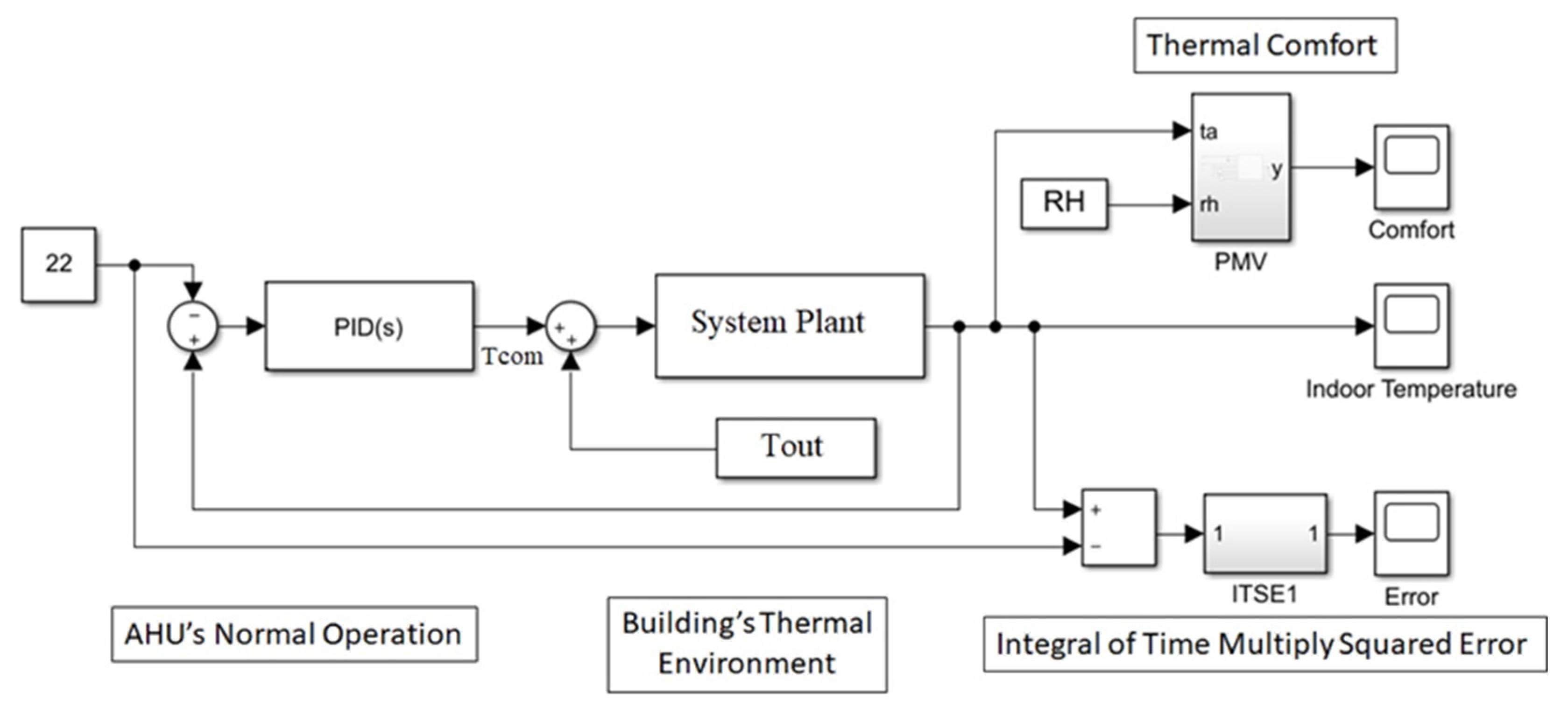
3.1. Modelling of ACMV Systems with Thermal Comfort

The usage of ACMV systems directly affects the thermal environment; therefore, the correlation study between both subjects will offer an important perspective. The selection of data from temperature sensors and thermal comfort methods is significant to illustrate the relationship between outside and inside temperatures. The initial step in creating this ACMV system model is to choose a location. The building site selection criteria for data collection purposes are discussed. Many factors are considered when selecting a site, including the building’s condition and the cooling system applied. The second step is to verify that the placement of the temperature sensors set in the building is comprehensive and capable of providing correct information on the temperature conditions in all areas of the building when the ACMV system is engaged.
Next, the preparation of the necessary data for inclusion in the simulation model should be recorded. Outdoor temperature, weather conditions, current humidity, and indoor temperature should all be logged or obtained from trustworthy sources. Finally, the application of nonlinear ARX algorithms in the generation of simulation models will be discussed in depth. This method is used to explain mathematically how the cold air produced by the ACMV responds to the ambient temperature conditions within the building, which are affected by the hot temperature outside the structure.

3.2. Temperature Sensors Placement

The place of investigation can be defined as a location and circumstance where researchers hope to be able to record the building’s current condition for gathering data. As a result, the location, timing, and environment were chosen to gather the required data in line with the objective of the study and obtain the correct results. The gold certification of the MITI Building by the GBI, whose accreditation body was founded by the Malaysian Institute of Architects in 2008, was an important consideration in the location’s selection. The building’s interior was equipped with thermal and humidity sensors that were used to gather information about the performance of the ACMV systems. As a prerequisite for the GB Index to acknowledge the MITI building as a gold standard, the building has a BAS that can record all pertinent data connected to the accreditation, which includes temperature, humidity, usage of energy, and quality of air data. The position of the sensors is depicted in Figure 4.
Figure 4 shows a layout with temperature sensors positioned throughout the space, and the number indicates the quantity of temperature sensors in that space. The front, inner, and rear spaces are where most of the data collected for research purposes is concentrated. One AHU, designated AHU-L31-1, cools the floor at the selected level and, when turned on, serves to keep the environment in the area at a comfortable temperature. The placement of all 12 sensors completes the cooling management system for the building’s internal area. Based on the size of the room and the shape of the space, the number of sensors in each designated room varies. Each room includes a VAV system that acts as a diffuser for the cooled air coming from the AHU into the room [47].
Most sensors indicate a drop in temperature; however, there are those that show an increase in temperature. The position of the room, which experiences the phenomenon of sunlight changing as it rises from the east and sets in the west at dusk, influences the increase and decrease in room temperature. However, there are times when the ambient temperature drops below the setting level. This is due to the room’s location in the centre of the building, which is shaded from the sun, enabling radiant heat to have little impact on temperature fluctuations. The graph illustrates that there is a variation in the effect of sunlight on the internal temperature of the structure, which causes the cooling system to operate in unequal circumstances since there are places that need a lot of energy to cool and spaces that do not require any cold air. Each sensor’s average temperature reading, divided according to the sensor’s location, is shown in Figure 5.
The strategically placed sensors in a structure’s environment collect extensive data on the surrounding temperature in addition to the duration needed for the AHU to regulate the area’s temperature up to the appropriate level. The crucial areas with the biggest effects on energy use are highlighted in Figure 5. In comparison to the core space, the average measurements in the upper part and rear sections are much higher. This demonstrates that the internal space’s temperature has a smaller impact on temperature fluctuations. The sensors utilized to calculate the average interior temperature of the structure are those in the upper and rear areas. This study applies quantitative methods and cluster sampling for data collection to inspect the effectiveness of the ACMV for controlling the effect of outside temperature on the inside structure’s climate. Figure 6 displays a block diagram of the data acquisition system.
A country such as Malaysia, which lies on a latitude that has a humid climate the entire year, just has two types of meteorological conditions. Therefore, the data can be split into two separate groups: wet (rainy) days and dry (no rain) days.
Throughout the year 2018, the days in which the water level measured from ground level were 0 mm for the period from 8 a.m. to 8 p.m. are listed in Figure 7. The highest and lowest temperatures for each month are also shown. The ambient temperature was recorded to be between 22.5 °C and 34.6 °C, providing a vivid picture of temperature measurements on bright days. Figure 8 depicts the temperature condition within the building due to the external ambient temperatures, while Figure 9 illustrates the building’s temperature state throughout the day without rain. The black dot line represents the temperature characteristic for each day, and red lines indicating the average temperature are added to both figures to help explain the temperature variances.
The temperature inside the building is low in the morning and slowly rises to its highest level at 15:00, like the outside. The temperature then drops as the day grows darker. The amount of water vapor in the air is known as humidity. Subsequently, cooler air contains more water vapor than warmer air and most water vapor is undetectable to the human eye. The likelihood of rain, dew, or fog is indicated by humidity, which is influenced by the system’s temperature and pressure. The maximal humidity at the same temperature is compared to the current absolute humidity to determine the relative humidity. Water vapor per volume of moist air or per mass of dry air is used to measure absolute humidity. ASHRAE recommends a humidity range of 45% to 55% to control health impacts and diseases.
Figure 10 and Figure 11 display the temperature and humidity of the building once ACMV is in operation, with the red mark indicating the average of the two parameters. The structure’s humidity level peaked in the morning and then stabilized at about 60% for the remaining of the day. Humidity readings are necessary for the PMV and PPV techniques of calculating occupant comfort levels. The temperature within the building also decreased, and after about an hour, depending on the temperature setting, the temperature could be maintained consistently via the ACMV system.
To prevent discomfort, respiratory issues, and an aggravation of allergies in building inhabitants, indoor temperature and relative humidity levels must be kept within a certain range. The symbol ΔT in Figure 12 depicts the temperature differential between the exterior and interior temperatures. The distinction between the two readings is minimal at 7.30 a.m., steadily rises throughout the day, then starts to reduce again as the day draws to a close. The inside temperature was recorded every 15 min, resulting in a daily average of 45 measurements. The declining and saturation trend in indoor temperature findings from the start of the day to the evening is indicated by the dotted mark in Figure 13 and embodies the total data’s average reading. The grayish zone, when compared to the average readings from all the data, is the middle point within the temperatures recorded at the highest and lowest points. The red mark displays the 22.2 °C temperature setting in this chart and expresses the idea that the most pleasurable selection of temperatures is within the grey area.
The structure is outfitted with an ACMV system that makes use of VAV technology. By controlling the appropriate volume of cold air circulation flow rate into the air-conditioning region, the VAV system delivers space cooling. Regardless of the necessity for chamber cooling, the supply chamber’s chilling air temperature is always maintained constant throughout the processing. However, the cold-water flow rate through the AHU coil will be adjusted depending on the space cooling need. Simultaneous adjustments made to the flow rate of water and cold air at low side loads require the process of dehumidification of supply air to take place inside the AHU boiler. Even if the cooling load changes due to the uneven structural characteristics of the space, the VAV system can adjust and maintain the temperature required by the space.
The present temperature scenarios dictate the fan’s speed; if an upsurge in temperature is identified, it will accelerate; otherwise, it will stay unchanged to uphold the ideal temperature. As a result, the power required by the fan is not constant but fluctuates according to the need to cool each room. To keep the temperature in space at a manageable level, the VSD, discharge dampers, and IGV control the air flow rate, which varies according to factors such as site conditions, space design, and surrounding temperature. The command temperature, as shown in Figure 14, is the cool air that the air conditioner produces, which adjusts the room’s ambient temperature to the desired temperature setting.
The T c o m graph shows how the typical temperature increases early of the day, drops sharply an hour later, then rises progressively the remaining hours of the day. The air temperature coming out of the diffuser is neutral when T c o m is high than when it is low. Figure 15 illustrates how the T o u t and T i n criteria are used to create the T c o m graph. T c o m will react to ensue T i n is within the designated temperature range when there is a disparity between T o u t and the planned temperature for T i n .
At time t 0 , whilst the ACMV system is activated, T o u t and T i n have already reached a particular value. T c o m adjusts its temperature to maintain the desired temperature in response to the discrepancy between T o u t and T i n as time approaches t 0 + 1 . T c o m then proceeds to supply input on the ensuing temperature difference at time t 0 + 2 to adjust the internal temperature of the building and continue doing so until the AHU is turned off.
Table 2 shows the symbols for mathematical Formulas (13) and (14), which were used to describe the room cooling process.
T i n t 0 = H T o u t t 0 + T c o m t 0 + 1
T i n t 0 1 = H T o u t t 0 + 1 + G T i n t 0

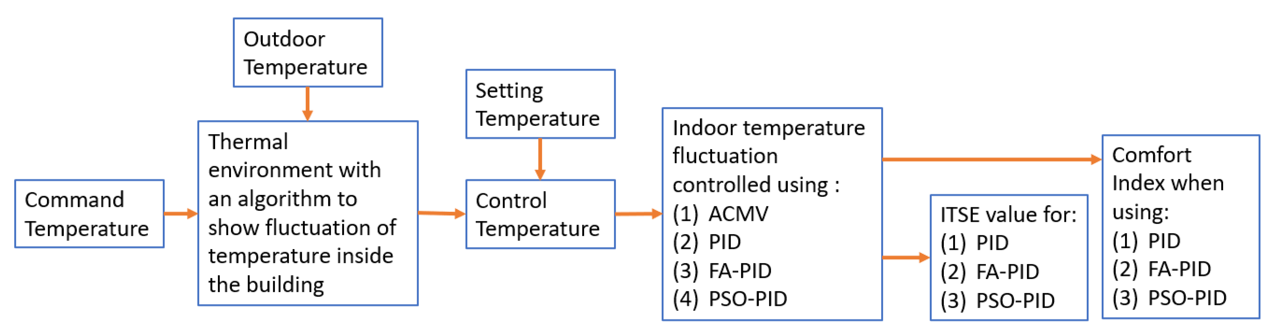
3.3. Simulation Model

Several parameters were utilized to create the simulation model for the building temperature close loop control system illustrated in Figure 16. The model is divided into four main parts that have different roles in forming a complete simulation system. The thermal environment of the building is addressed in the first part, and the normal operation of the AHU is covered in the second part. The third part is the error comparison, while the fourth part is devoted to thermal comfort.
The first section is in the middle of the simulation model, and it combines the system plant block equipped with an algorithm for displaying temperature fluctuations inside the building’s indoor area with the T o u t data and T c o m that acts as the block’s input. T o u t represents the outside temperature measurement from 7 a.m. to 6 p.m. on a non-rainy day while T c o m is a temperature measurement produced by the controller after it has processed the feedback loop’s input. Both pieces of information are entered into the plant’s block system.
The second section of the model consists of control system blocks that obtained its input from the take-off point established by the first section’s outcomes, as well as from the T s e t data. T s e t is a readout of the cooling system’s required temperature setting. The third section has two major components: the results of the building’s T i n conditions and the ITSE for each control system. T i n data are the indoor temperature readings taken throughout the day from 7 a.m. to 6 p.m. Four unique internal temperature readings reflecting four distinct kinds of controls are presented in this section.
The four different types of controllers consist of the original controller known as AHU, controller by tuned PID, PID controller optimized by PSO, and PID controller optimized by FA. The fourth part examines the impact of various temperature controls on occupant thermal comfort. The comfort is quantified using an index, with a higher value indicating a higher degree of pleasure with the ambient temperature perceived by the occupant.
There are two circumstances that must be addressed in the process of developing a simulation model that can represent the cooling process capable of maintaining comfortable temperature, respectively, when the cooling system is active and when it is not engaged. When the cooling system is deactivated, it is referred to as an open loop, and when the system is active, it is referred to as a closed loop. Figure 17 represents the simulation’s block diagram.
Formula when the system open loop is given as,
T i n t = H T o u t t
T C i n t   is not constant and varies with T o u t ( t ) , when the system close loop,
T i n t = H T o u t t T c o m ( t ) T C i n t = H ( T o u t t H T c o m ( t )
Assuming H is Linear Time-Invariant (LTI) and inversible, by definition, a closed loop should set T i n ( t ) to constant value T s e t such that,
H   T c o m ( t ) = H T o u t t T s e t T c o m t = H 1 T o u t t T s e t = H 1 H T o u t t H 1 T s e t = T o u t t H 1 T s e t
Note that T c o m t = G T i n t ,
G T i n t = T o u t t H 1 T s e t
The outdoor environment of a building affects its indoor heat gain and heat loss. Temperature data show that heating energy increases steadily inside the building from morning to evening and does not dissipate instantaneously when the AHU system is activated. This translates to a dependence in previous values of indoor temperature while AHU constantly operates to reach the setting temperature required. Equations for nonlinear diffusion can be utilized to regulate relative humidity and temperature in a space. Assuming the plant relating T o with T i is a non-linear autoregressive order-1 process given by the equation:
T i t = α T o t + β T i t 1 + γ
The consideration of the nonlinear ARX algorithm is that heat that enters the room does not simply vanish. The room temperature becomes high as time progresses, and the heat does not disperse immediately. This translates to a dependence on previous values of indoor temperature. The calculation of using order-1 approximation is an arbitrary choice: higher-order models can be used, but order-1 fit is very good on the average of T o and T i . Nonlinear ARX approximation tool is utilized to obtain all three constant values. Table 3 specifies the constant values for α ,   β ,   a n d   γ :
The decision to update any system must be made with caution because the execution of a change necessitates a significant financial investment. As a result, the proposed new system must provide convincing proof that its future deployment will be lucrative. Studies were carried out to further enhance the cold temperature management by ACMV systems, with the creation of a model capable of displaying the condition of the internal temperature character of the building in a manner comparable to the actual data. To characterize the temperature variations induced by ACMV control, this model was created by merging a PID control system with the NL-ARX algorithm. Temperature variations on non-rainy days were considered in this study to find the optimal control system for one type of situation at a time. Even when picked from the same weather circumstances, there are substantial disparities in the graph characters gathered because a day that is not wet does not always guarantee it will be sunny. There are situations where clouds cover the sky and cloudy weather conditions inevitably affect temperature fluctuations.

3.4. Optimization of ACMV Control System
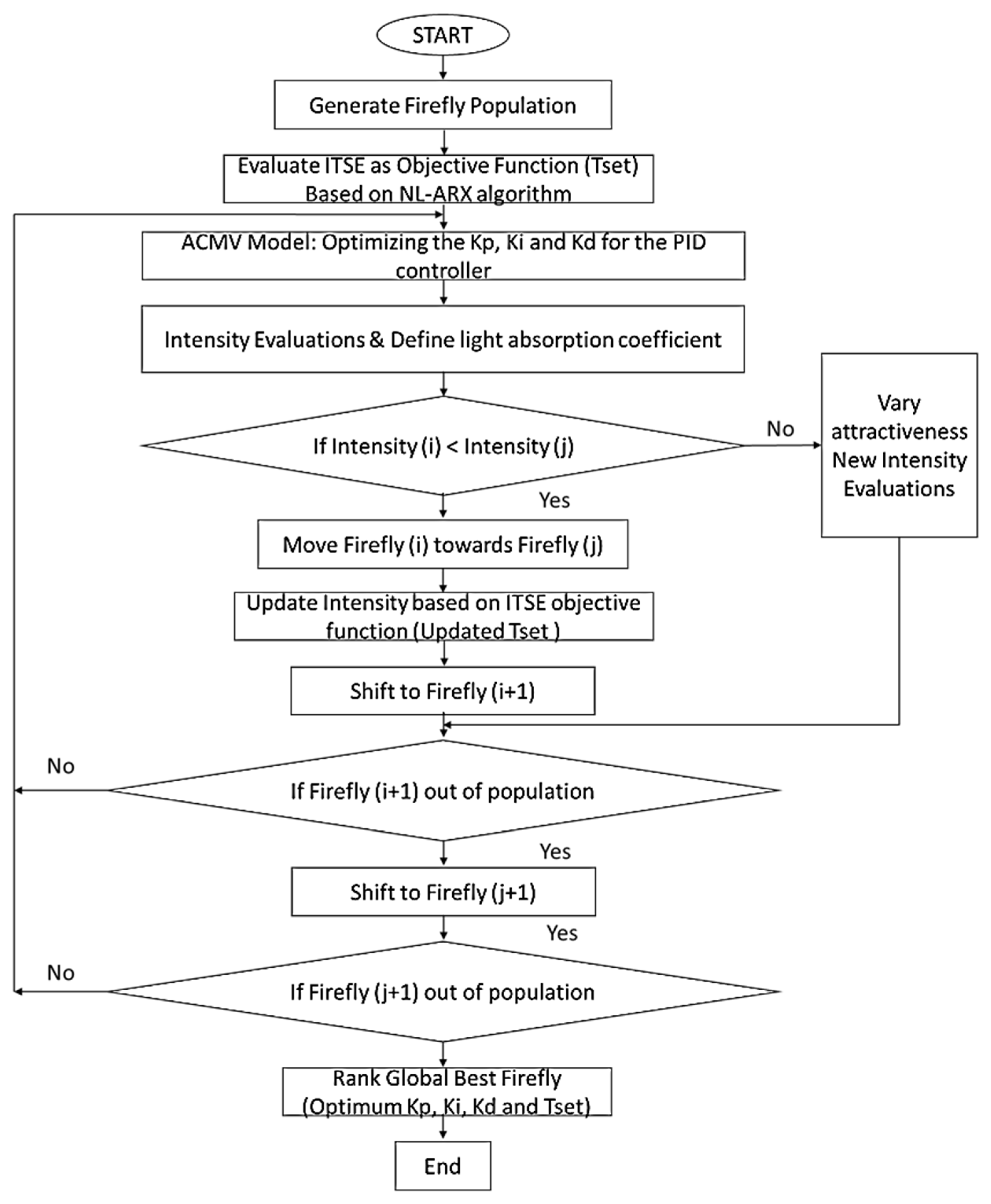
The optimization issues in this thesis essentially include the development of a control method to adjust the indoor temperature to remain at the desired setting while achieving energy efficiency and comfort in smart buildings with an ACMV cooling system. The emphasis is on control system efficiency since centralized ACMV systems use a lot of energy. Furthermore, the assured indoor air quality, which has an important influence on occupant wellness and work efficiency, is managed and maintained by ACMV systems as well. As a result, the optimization issues are narrowed down to regulating the ACMV system to be more efficient in achieving temperature stability in the building at a quicker and more accurate rate while enabling the occupant to experience a pleasant temperature while within the building.

3.4.1. FA

The reaction of fireflies to their surroundings inspired the development of the FA, a Metaheuristics optimization approach. The brighter the light generated, the greater the attraction, and the fireflies that create the dimmer light will come closer to the fireflies that produce the brighter light. However, if all the light brightness is the same, the fireflies will travel at random [57]. This idea of fireflies’ behavior inspired the development of the FA. This algorithm has three fundamental rules:
  • Fireflies, whether male or female, will constantly emit light to attract one another;
  • The fireflies’ attraction is proportionate to their brightness. As a result, fireflies are drawn to and migrate in response to greater levels of light. As the distance between two light rises, the intensity of the light reduces;
  • The resultant brightness level indicates the objective function’s value.
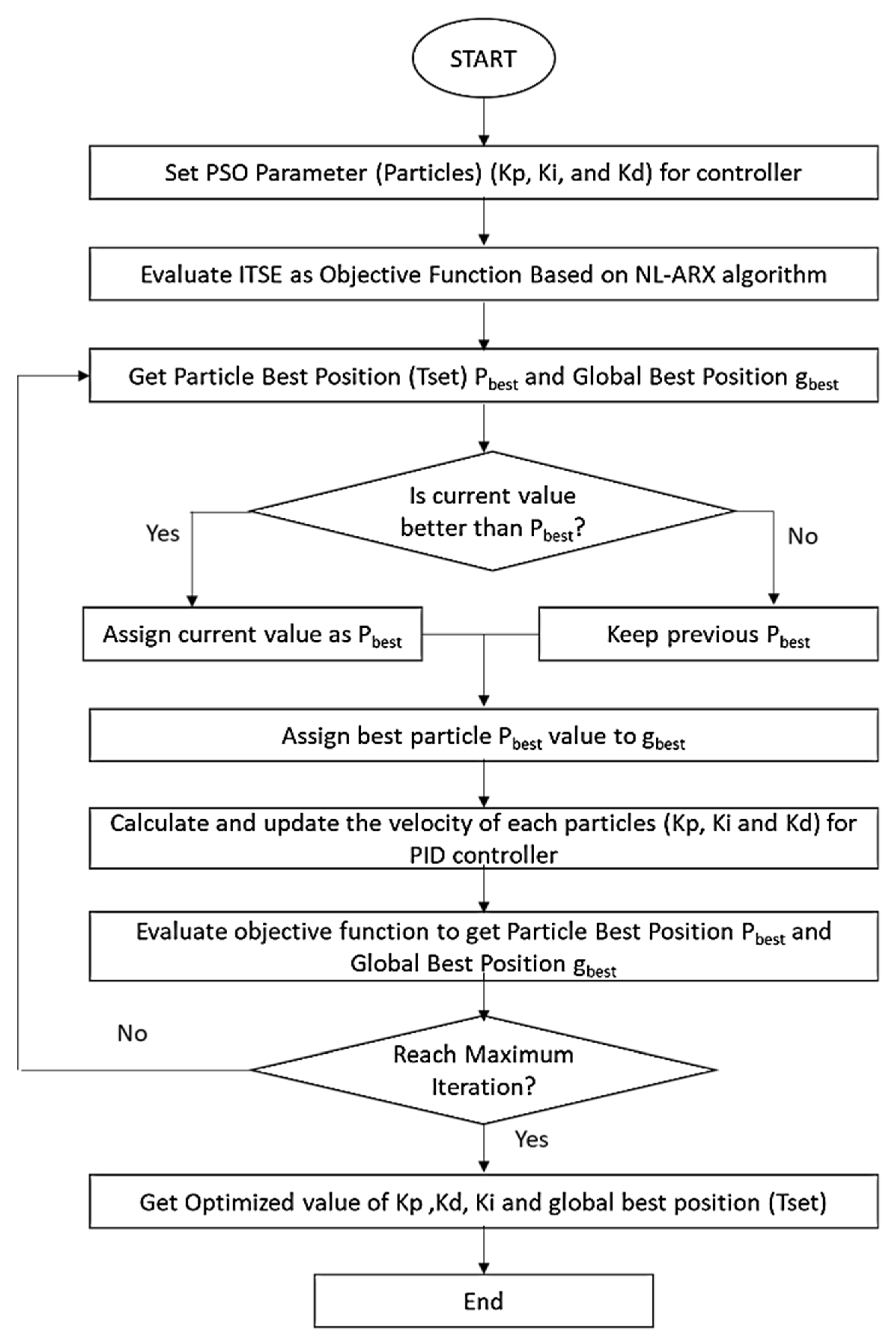
Figure 18 illustrates the FA flowchart.
The firefly’s attractiveness β as a function of distance (r) is defined as follows [58]:
β r = β 0 e γ r 2
where β 0 represents the attractiveness at r = 0 and γ is the constant light absorption coefficient. The Euclidean distance is used to calculate the distance between any two fireflies r i j :
r i j = x i x j = k = 1 d x i , k x j , k 2
where x i and x j represent two separate fireflies and the movement of the fireflies is denoted as:
x i = x i + β 0 e γ r i j 2 x j x i + α r a n d 0.5 × s c a l e
where is the randomly generated variable and r a n d are a random figure generated between 0 to 1. The scale is utilized as the scaling parameter, with the value spanning the top and lower bounds. The following are the usual values used in this study: β = 1 , γ = 1 , and α = 0.8 . The fireflies are used to denote the PID parameter K p , K i , and K d in the controller optimization problem. The error criterion of the controller expressed by the ITSE is used as the objective function.
I T S E = 0 t t · T s e t 2 d t

3.4.2. PSO

PSO is one of the algorithms designed for computers to be able to calculate using a certain quality measure repeatedly to identify the ideal response to a particular concern. The challenge is handled by producing a population known as a particle and shifting these particles throughout the search domain via a mathematical algorithm formula based on velocity and position. The best-known local position governs the motion of each particle; however, if another particle discovers the better-known point in the search, the location is updated, and each particle is routed to that location. It is adapted by the movement of groups of birds that fly together randomly but organized and do not crash into each other, creating the illusion that they are all flying in one huge search region. The PSO approach does not make any assumptions to discover a solution to a problem.
PSO is distinct from other traditional optimization methods, such as genetic algorithms and gradient descent methods since it does not need difference in optimization or optimized gradients of the problem. PSO has its foundation according to the swarm particle’s social conduct. By changing an objective function, this method locates and determines the global optimum answer. At the conclusion of the procedure, the optimum solution for two degrees of freedom PID controller settings in accordance with objective function is determined. PSO selects random solutions to populate the population to start the process. Then, to obtain the best value, it upgrades its performance. Every particle in the swarm is defined by its location and velocity. A moving particle’s velocity is affected by changes in location or direction. The two components p b e s t and g b e s t , which stand for the particle’s ideal positioning and the swarm’s overall best position, are used by each particle to determine its new location. The PSO’s flowchart is shown in Figure 19.
Equations (24) and (25), respectively, may be used to describe the particle’s velocity and location [58].
v i j t + 1 = w v i j t + r 1 c 1 p i j t x i j t + r 2 c 2 g j t x i j t
x i j t + 1 = x i j t + v i j ( t + 1 )
W stands for inertia weight and is used to accelerate PSO convergence; it typically has a value between (0, 1). The velocity of particles is represented by v i j t , c1 and c2 are acceleration coefficients, and r1 and r2 are random integers between (0, 1). Typically, c1 = c2 = 2 and x i j ( t ) is added to record the current locations of all particles in all dimensions. v i j ( t + 1 ) and x i j t + 1 are particle updated velocity and position, respectively. Parameter p i j t is the particle best position, while g j t is the global best position of the swarm. The PSO method begins by initializing the swarm range, location, velocity, and the variables w, c1, and c2. Then, the fitness value of each particle is then computed, p b e s t and g b e s t are specified, and each particle’s location and velocity are changed. When the halting condition is fulfilled, the algorithm comes to a halt. The best solution is selected based on the most recent g b e s t . Table 4 shows the PSO parameters and their values that were utilized in this research.
There are two circumstances that the controller must overcome to be a benchmark for the controller’s performance; specifically, the controller must be able to quickly achieve a preset temperature setting and keep the Tin temperature constant throughout the controller’s active period. In this research, the FA-PID is compared to the other two controllers, which are the traditional PID controller and the PSO-PID. The built-in PID controller in MATLAB was utilized as the traditional PID controller in this study.
Similar outcomes in temperature control optimization can also be attained by using the MPC control approach, which selects control inputs to optimize a specific objective function using the fluidity of a system to forecast future behavior. In addition to MPC, the FLC control approach is efficient at dealing with nonlinear systems and uncertainties because it makes use of linguistic variables to define system behavior and control objectives.

4. Results and Discussion

The developed model of an ACMV system with thermal comfort index compares temperature management techniques that could improve indoor temperature stability and occupant thermal comfort sensation. Furthermore, the model also comprises a thermal comfort algorithm to demonstrate the effect of temperature management on the building’s occupants. The algorithm for thermal comfort sensation is based on the well-known ASHRAE Standard 55-2020 developed by Fanger’s PMV-PPD model, which is also classified as a passive approach that relies on ecological variables to assess the occupants’ thermal convenience [59]. This chapter covers two important research outcomes on indoor temperature control and comfort assessments, both of which were shown using simulation models based on available data obtained from the MITI building.
The simulation model was developed using a tuned PID controller to have the same disposition as the ACMV cooling system. The non-linear ARX algorithm, which can capture the dynamic behavioral temperature variations that occur inside the building space, serves as an identification system in the modelling plant. The PID controller was then adjusted to include two types of nature-based optimization, FA and PSO, as an alternative to improve and enhance control quality. These two types of control methods are named FA-PID and PSO-PID, respectively. The three types of controllers, namely, PID, FA-PID, and PSO-PID, were then compared to evaluate the effectiveness of their control performance against the AHU controller from the ACMV system. The comparison of all types of controls involved was performed over 40 different scenarios.

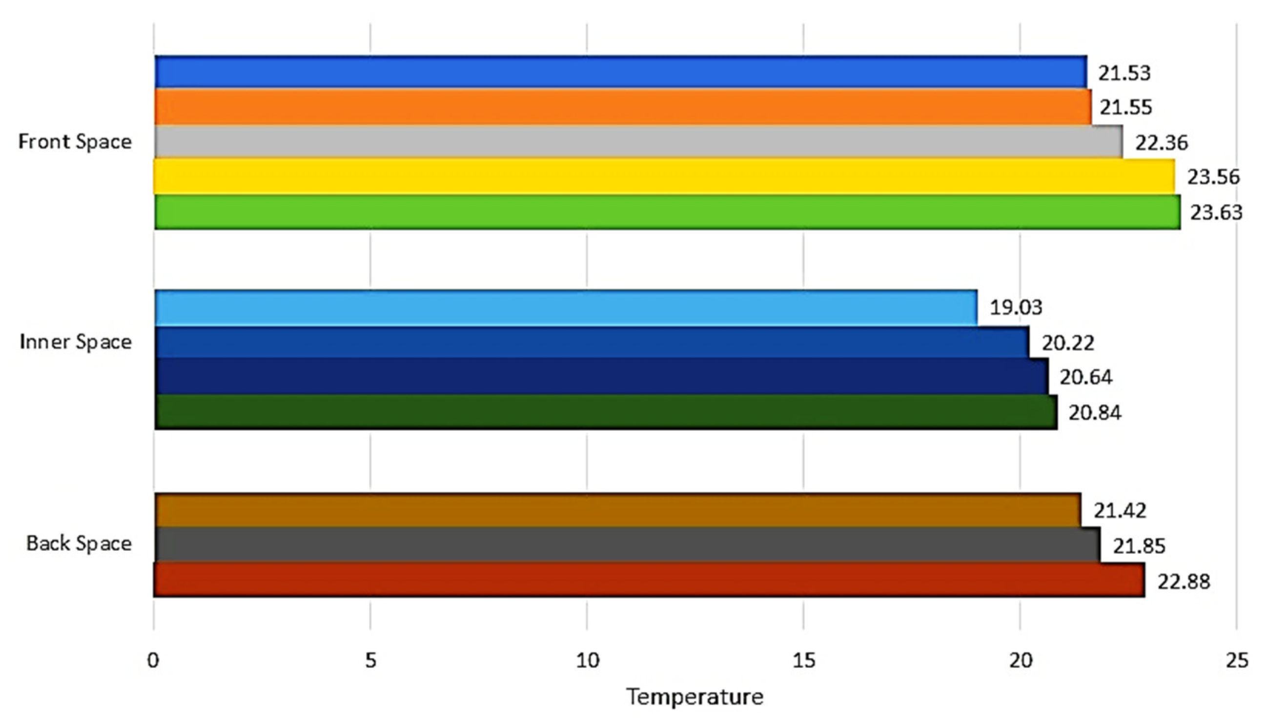
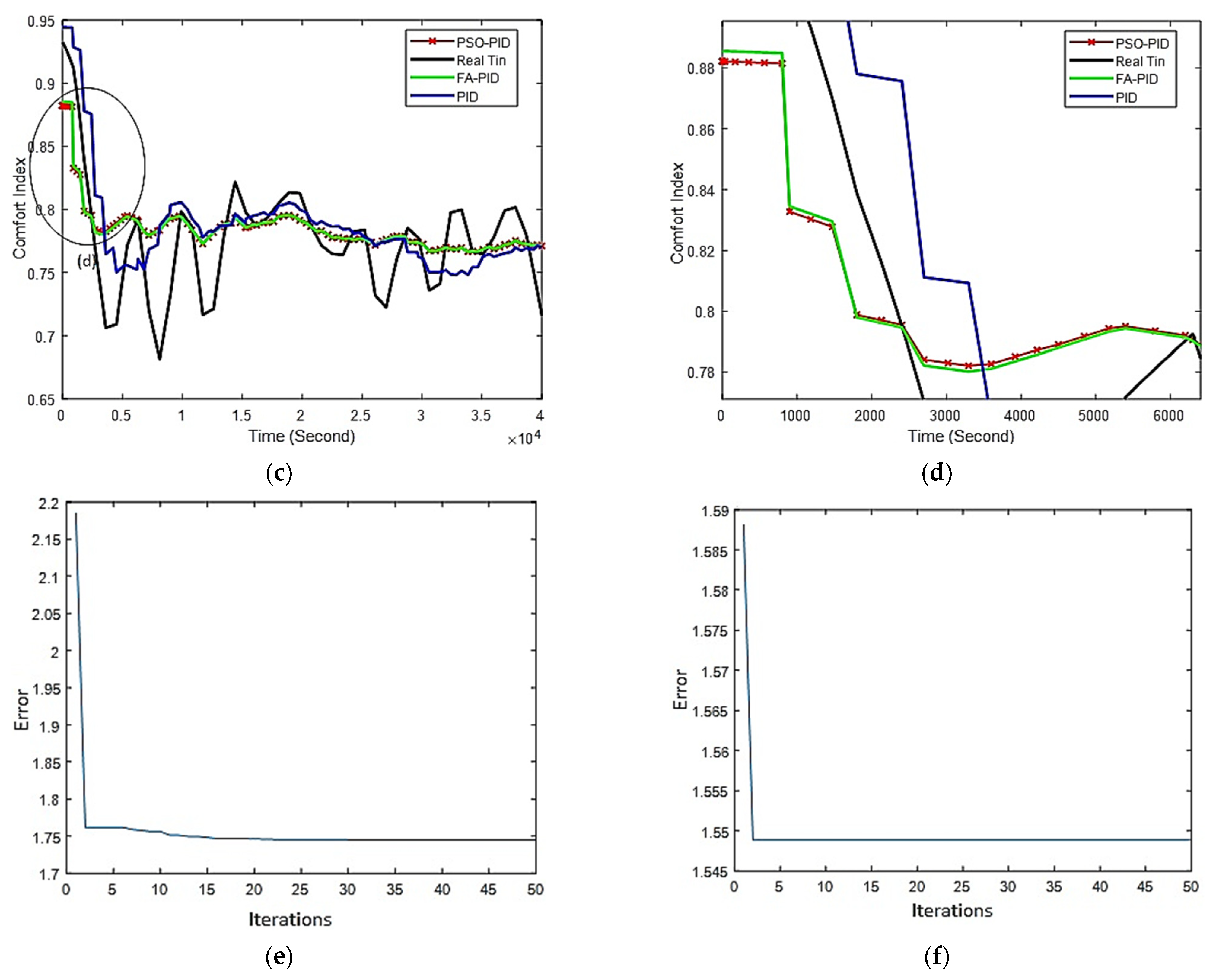
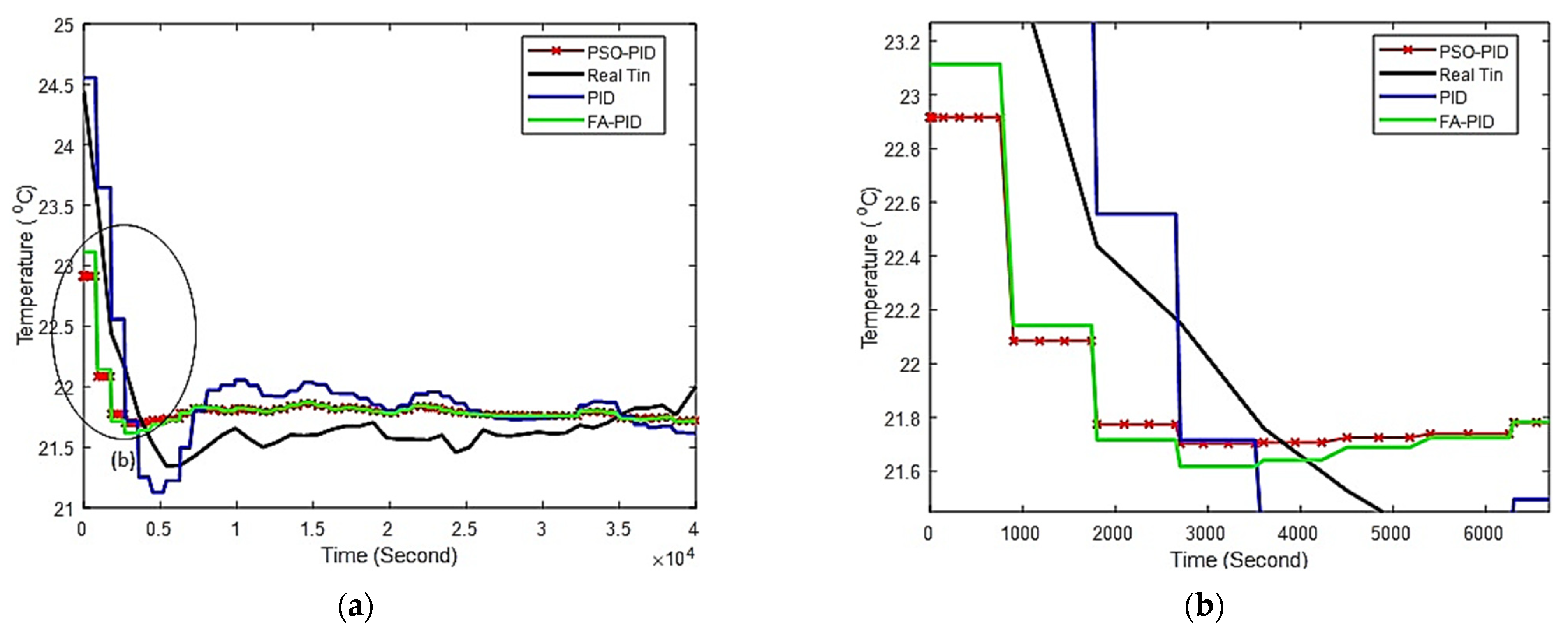
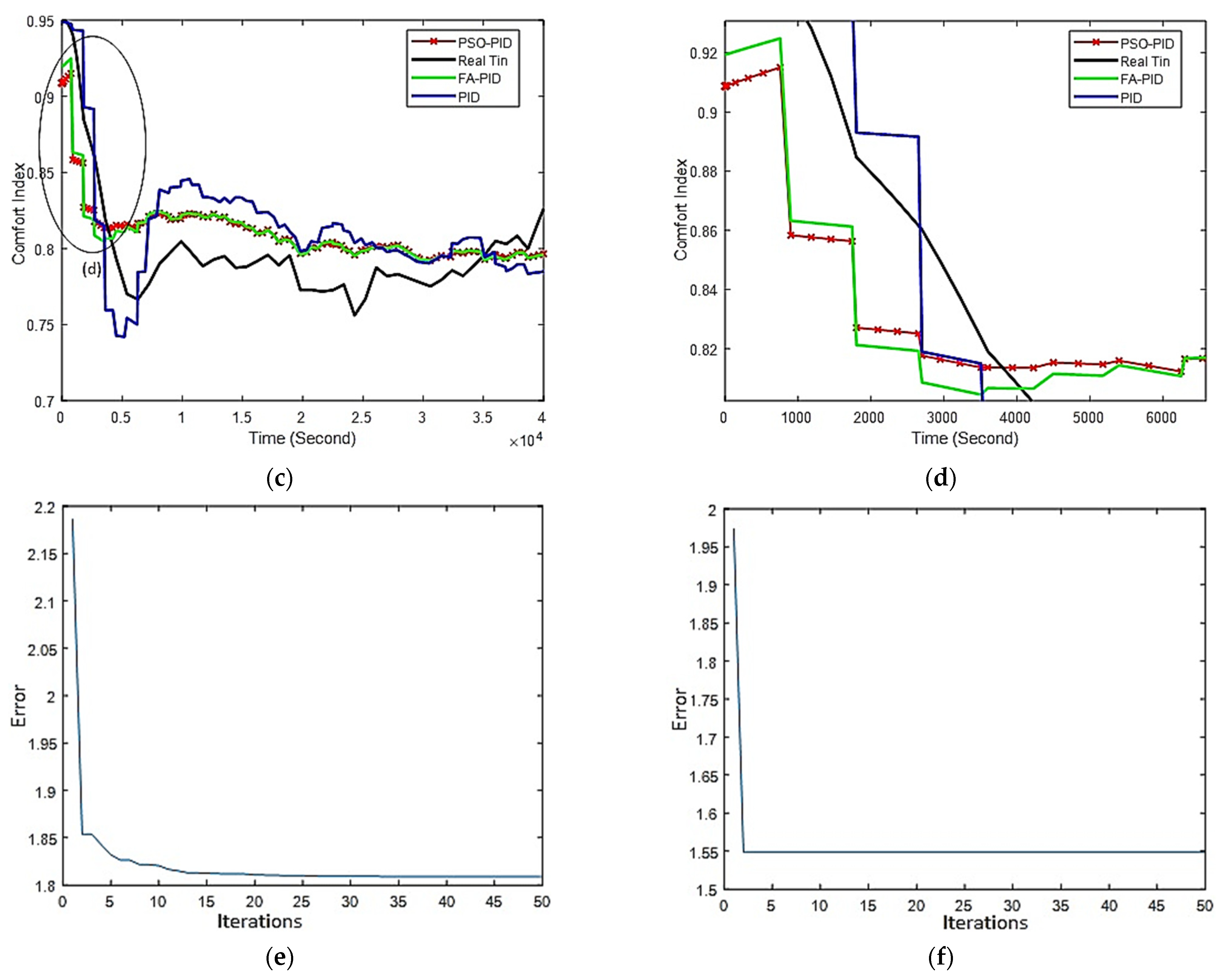
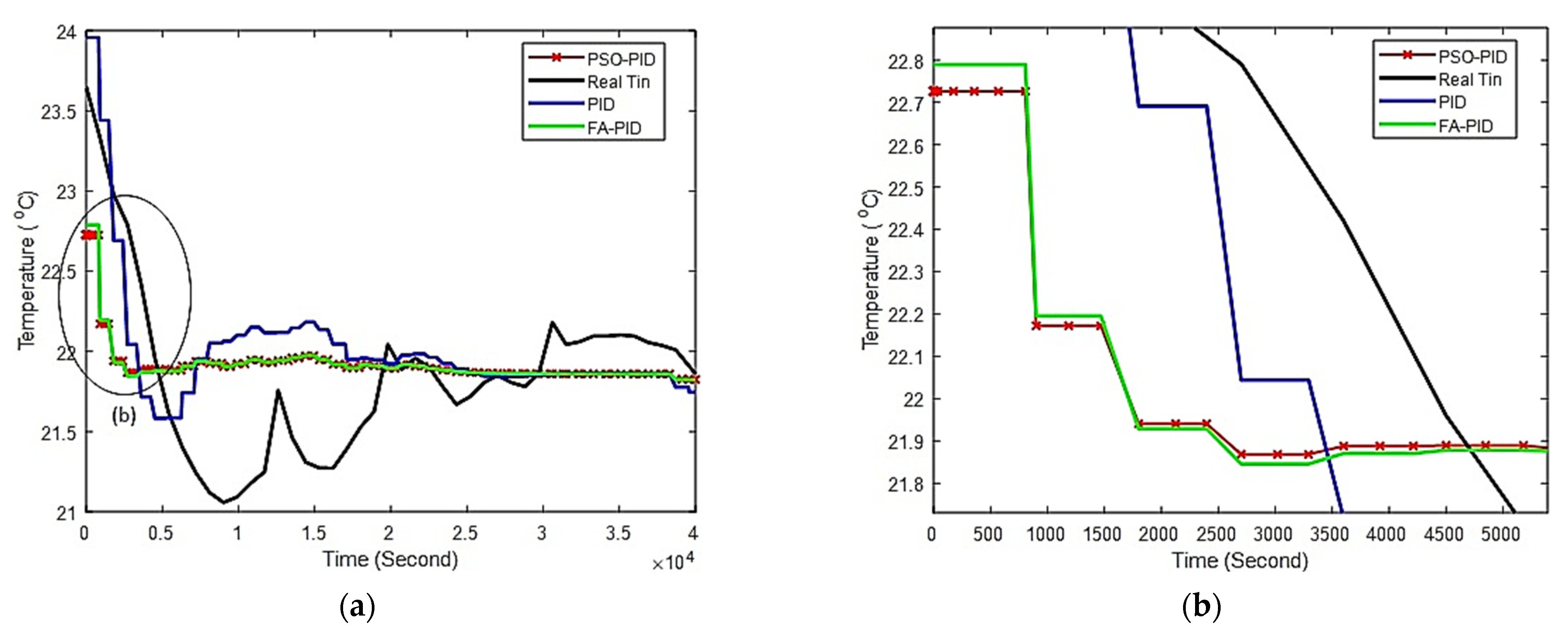
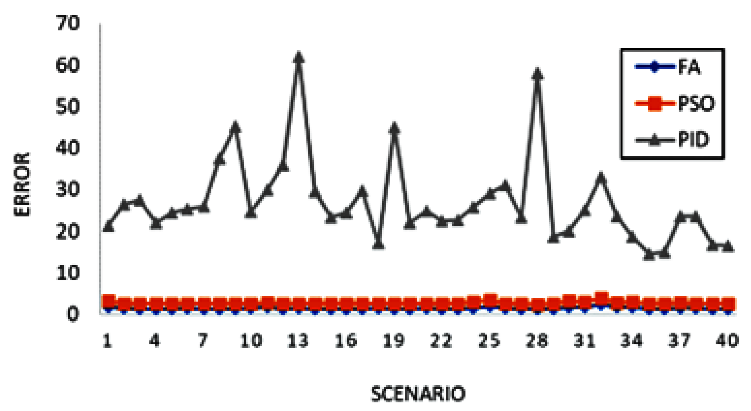
4.1. Result Analysis

Three data points are chosen out of forty data points to analyze controller efficiency. Each point represents the indoor temperature settings, T s e t , that has been altered based on outdoor meteorological conditions on that day to achieve thermal comfort. All 40 scenarios with varied temperature settings are illustrated in Figure 20. The red trendline drawn using the polynomial technique indicates the trend of temperature setting ranged between 22 °C and 22.5 °C.
The temperature setting spans from 21 °C to 24 °C. Figure 21, Figure 22 and Figure 23 show a comparison between four controllers in terms of control performance and comfort index conditions due to different controls techniques. The black circle indicates the part that will zoom in on the next figure. The finest control technique is determined by the controller’s capacity to keep the building’s indoor temperature readings at the specified T s e t with low oscillatory rate. Convergence graphs of FA-PID and PSO-PID are also shown for comparison in finding the minimal error. The actual indoor temperature serves as a gauge for the effectiveness of the AHU controller installed in the structure. A PID controller emulates the AHU by using the system identification technique in simulation.
The tuned PID values for air handler for this case are K p = −2.482, K i = −0.002932, and K d = 1870.809. The findings emphasize performance comparability between FA-PID and PSO-PID as can be seen from Figure 21b,d where the graphs of controller and its comfort index were being enlarged over the first 5000 s to highlight the difference between both optimized PID controller. The resulting thermal comfort from all four distinct types of controllers were calculated using the PMV approach, which is compliant with ASHRAE Standard 55-2020.
An index form of 0 to 1 is used to measure the thermal comfort. The comfort range values for each controller are compared to verify its stability and dependability. The range is the distance between the graph’s highest and lowest points. Lower range indicates better thermal comfort and sensational stability. The convergence graphs of FA-PID and PSO-PID indicate the number of iterations for particles and the maximum generation for fireflies before the curve becomes stagnant or saturated, indicating that the lowest error has been attained. The number of fireflies and particles being used in this study is 20 with 50 iterations. The ITSE approach is used to evaluate the controller performance by calculating the error between the obtained graph line and the desired temperature setting. The outcome is displayed as an index value.
The first scenario data in Figure 21 were taken from day 1 of a dry-day condition with T s e t = 21.47 °C. The range difference between the minimum and highest points of the four interior temperature readings is depicted in Figure 21a,b, with the AHU controller having the largest range of 2.52 °C. The median temperature was kept at 21.53 °C by the PID controller, whereas the median temperature was measured at 21.5 °C for the FA-PID and PSO-PID controllers. The actual indoor temperature had the lowest median comfort measurement of 0.7817, while the PID controller had the greatest median comfort measurement of 0.7865, according to Figure 21c,d. In comparison to the FA-PID controller, the PSO-PID controller achieved the least comfort range of 0.1154. The PSO-PID method converged quicker than the FA-PID approach, as seen in Figure 21e,f.
The second scenario data are selected from day number 25 of a dry-day condition with T s e t = 21.76   °C . Figure 22a,b illustrates the range difference between the minimum and maximum points of all four indoor temperature reading with PID controller having the biggest range, of 3.428 °C. The PID controller managed to keep the median temperature at 21.87 °C, while the FA-PID and PSO-PID controllers had the same median temperature measurement of 21.8 °C.
Based on Figure 22c,d, the real indoor temperature had the lowest median comfort measurement at 0.7928 while PID controller had the highest median comfort at 0.8141. The PSO-PID controller managed to obtain the smallest comfort range at 0.1229 compared to 0.1328 for the FA-PID controller. Figure 22e,f indicates that the PSO-PID algorithm converged faster than the FA-PID algorithm.
The third scenario data are from day 30 of a dry-day condition with T s e t = 21.86 °C. Figure 23a,b depicts the difference in range between the minimum and highest points of all four interior temperature readings, with the AHU controller having the largest range of 2.59 °C. The PID controller managed to hold the median temperature at 21.95 °C, while the FA-PID and PSO-PID controllers both had the same median temperature measurement of 21.9 °C. According to Figure 23c,d, the true interior temperature had the lowest median comfort measurement of 0.8071, while the PSO-PID and FA-PID controllers both had the greatest median comfort measurement of 0.816. The PSO-PID controller achieved the least comfort range, 0.1117, compared to 0.1154 for the FA-PID controller. Figure 23e,f shows that the PSO-PID method converged quicker than the FA-PID approach. The ITSE computation is used to determine controller validation, and Table 5 presents the findings.
According to the results shown in Table 5, in comparison to the FA-PID controller, the PSO-PID controller had a lower ITSE value. The ITSE value for PSO-PID was in the range of 1.549 to 1.598, which is better than the FA-PID controller that had an ITSE value range between 1.707 and 1.809. This result indicates that PSO-PID is the better controller for all three selected scenarios.
According to results obtained from experiments, assessments, and validations of models shown in Figure 21, Figure 22 and Figure 23, the control technique used in this research was successful in making the temperature control more stable than the original control. These findings are critical in demonstrating that changes have been made to further enhance the quality of current controls. It offers compelling proof that the PSO-PID optimization control strategy is successful in improving the standard of temperature management in indoor spaces.
Not only does the new control performance effectively regulate the temperature, but it also successfully reduces the time needed to achieve the target temperature. Faster temperature control can be seen in all the results shown. For example, in scenario 1, the original temperature control took a long time to stabilize the temperature, but it continued to fluctuate until the end of the control period and failed to maintain the desired temperature when compared to controls performed by tuned PID, FA-PID, and PSO-PID, which take less time to reach, and stabilize at, the desired temperature.
PMV and PPD indices forecast a large group of people’s average climate assessment value and the proportion of persons who would be unsatisfied with a given ambient environment, respectively. Results show the satisfaction index of the inhabitants against the temperature of the interior atmosphere of the building. Based on the results, occupants are steadily receiving comfort satisfaction without having to endure a state of precarious satisfaction when the temperature fluctuates.
In contrast to other control techniques presented in this research, the PSO-PID optimization control approach offers a better and higher level of comfort to the occupant. The comfort index is dependent on the circumstance and is tied to temperature settings, which somewhat vary for each individual scenario. The overall average comfort median value is 0.8689, suggesting that occupant contentment with the temperature consistency offered is quite high. Nonetheless, the occupant will still obtain maximum satisfaction due to the temperature stability provided.
Convergence graphs are used to determine that a measured quantity has converged satisfactorily. The graphs produced by the optimization process demonstrate good measure convergence as the curve becomes asymptotic when it plots data for the final iteration and generation. The results of convergence graph depict how the strain of error in a model converged with each iteration of the particle swarm algorithm and each generation of the firefly algorithm. Minimum error values are saturated as of the final iteration and generation, indicating that the convergence process is completed. In general, the findings of this study are encouraging, with the potential to considerably improve the quality of temperature regulation in interior environments, resulting in better occupant comfort and satisfaction.

4.2. ITSE Value Comparison between PID, FA-PID, and PSO-PID

The time-integral criteria are general and all-encompassing instruments for assessing the performance of a control system. There is an inherent purpose to decrease error in every feedback control system, and so a performance measure in terms of Integral of Time Multiply Squared Error (ITSE) is developed to always keep track of the mistakes from zero to infinity, and to eliminate them constantly. Error will be minimized if performance measures are kept to a minimum because error cannot be negative, and these performance metrics are usually stated in terms of either absolute value of error or square error. The error comparison between the PSO-PID, FA-PID, and PID controllers used in this model is shown in Figure 24. The ITSE calculation between each controller and the required temperature is used for this comparison. The T s e t is the target temperature, which varies depending on the scenario. A good outcome will provide a low error value, while a poor result will result in a high error value. A low error value means that the controllers can regulate the temperature close to the desired setting.
The PSO-PID control demonstrates a low error value compared to FA-PID with average error values of 1.27 and 1.39, respectively. The ITSE value for PID is extremely high when compared to FA-PID and PSO-PID. This demonstrated controller with improved optimization techniques is remarkably effective in aiding the improvement of the temperature control efficiency of existing ACMVs. Although the FA-PID controller seems to be satisfactory, the resultant error value is greater than that of the PSO-PID controller. In conclusion, the PSO-PID controller is the optimal control choice for the building’s indoor temperature control model. Comfortable indoor temperatures may very well be achieved with effective temperature control.

5. Conclusions

The study focuses on improving the ACMV control system to achieve comfortable temperature conditions in a building. Temperature readings were collected from sensors installed within the building space and outdoor temperature data were obtained from the Malaysian Meteorology Department. The collected data were categorized into rainy and non-rainy days. A simulation model was used to analyze the indoor temperature characteristics for non-rainy days and develop effective temperature control techniques.
The main parameter of interest is indoor temperature, but other parameters such as relative humidity and electrical power consumption were also considered. The study utilized a PID control technique to model the ACMV system and NL-ARX algorithm to analyze indoor temperature fluctuations influenced by outdoor temperature and cooling system emissions. The study also created a comfortable temperature index model based on ASHRAE standards to monitor the comfort temperature index concurrently with the current temperature conditions. Control performance evaluation involved four types of control: actual ACMV controller, tuned PID controller for simulation purposes, FA-PID controller, and PSO-PID controller.
The study incorporated FA and PSO algorithms into PID control to achieve quicker and more consistent results. FA is based on the attraction of brighter firefly lights, while PSO involves particles moving to converge at the best position. These optimization algorithms are widely used in studies on comfortable temperature control. The desired indoor temperature for the building was set at around 22 °C with a relative humidity of 60% to maintain a comfort index of 0.8 or higher.
The comparisons of FA-PID and PSO-PID controllers revealed that they delivered identical values for temperature but were distinct in how the comfort index value was controlled. The PSO-PID controller performed better in terms of keeping index difference values within a narrower range and lower ITSE values. The study showed that the PSO-PID optimization method outperforms FA-PID in terms of thermal comfort.
Nonetheless, the paper proposes three modeling-based temperature control strategies for optimizing ACMV control systems. It is useful for building managers and ACMV system designers who seek to optimize temperature control in buildings. The study was conducted in a single building for one year, but the findings are applicable to other buildings or places with varying environmental conditions.
The study focuses solely on temperature control and comfort index, without considering other elements that may influence the way the ACMV works, such as energy consumption and indoor air quality. Finally, based on recent developments in the research area, the study considers two optimization techniques, FA and PSO, in conjunction with PID control.

Author Contributions

Conceptualization, M.A. and K.K.; methodology, M.A.; software, H.K.A.; validation, K.V., K.K. and H.K.A.; formal analysis, H.K.A.; investigation, M.A.; resources, M.A.; data curation, M.A.; writing—original draft preparation, M.A.; writing—review and editing, M.A.; visualization, M.A.; supervision, K.K.; project administration, K.V.; funding acquisition, K.K. All authors have read and agreed to the published version of the manuscript.

Funding

This research and the APC was funded by Universiti Kuala Lumpur (UniKL).

Data Availability Statement

Data is available at Ministry of International Trade and Industry (MITI) Malaysia and Malaysian Meteorological Department.

Conflicts of Interest

The authors declare no conflict of interest.

Nomenclature and Abbreviations

Nomenclature
MMetabolic energy production, W/m2
WRate of mechanical work, W/m2
TaAmbient air temperature, °C
TrMean radiant temperature, °C
QdiffHeat loss via diffusion, W
QevapHeat loss via evaporation, W
QrespHeat loss vis respiration, W
fclClothing surface area factor
TTemperature, °C
varRelative air velocity, m/s
lclBasic clothing insulation, clo
rhRelative humidity, %
PaWater vapour partial pressure, (Pa)
hcConvective heat transfer coefficient, W/(m2·K)
Abbreviations
ACMVAir-Conditioning and Mechanical Ventilation
AHUAir Handling Unit
ARXAutoregressive Exogenous
ARIMAAutoregressive Integrated Moving Average
ARMAXAutoregressive Moving Average Exogenous
ASHRAEAmerican Society of Heating, Refrigeration, and Air Conditioning Engineers
BASBuilding Automation System
CDWPCondenser Water Pump
CHWPChilled Water Pump
FAFirefly Algorithm
FA-PIDPID controller optimized by Firefly Algorithm
FCUFan Coil Unit
GAGenetic Algorithm
GBIGreen Building Index
HVACHeating, Ventilation, and Air-Conditioning
IGVIntake Guide Vanes
ITSEIntegral of Time Multiply Squared Error
METMalaysian Meteorology Department
MITIMinistry of International Trade and Industry
NL-ARXNonlinear Autoregressive with Exogenous
NNARXNeural Network-Based Nonlinear Autoregressive
PIDProportional, Integral and Derivative
PMVPredicted Mean Vote
PPDPercentage of Dissatisfied
PSOParticle Swarm Optimization
PSO-PIDPID controller optimized by Particle Swarm Optimization
SCHWPSecondary Chilled Water Pump
T c o m Command Temperature
TinIndoor Temperature
ToutOutdoor Temperature
T s e t Setting temperature
ΔTTemperature Difference
vRelative Airflow Velocity
VAVVariable Air Valve/Volume
VSDVariable Speed Drive
WRate of Mechanical Work

References

  1. Saber, E.; Tham, K.; Leibundgut, H. A Review of High Temperature Cooling Systems in Tropical Buildings. Build. Environ. 2016, 96, 237–249. [Google Scholar] [CrossRef]
  2. Jayamaha, L. Energy-Efficient Building Systems; McGraw-Hill: New York, NY, USA, 2006. [Google Scholar]
  3. Ho, J.; Jindal, G.; Low, M. Singapore’s Intended Nationally Determined Contribution for Cop21 Climate Conference in Paris; Energy Studies Institute: Singapore, 2015. [Google Scholar]
  4. Hassana, S.; Zinb, M.; Majid, A.; Balubaida, S.; Hainina, R. Building Energy Consumption in Malaysia: An Overview. J. Teknol. 2014, 7, 33–38. [Google Scholar] [CrossRef]
  5. National Environment Agency. Stricter Energy Performance Standards for Air Conditioners; NEA: Singapore, 2016. [Google Scholar]
  6. Katili, A.R.; Boukhanouf, R.; Wilson, R. Space Cooling in Buildings in Hot and Humid Climates—A Review of the Effect of Humidity on the Applicability of Existing Cooling Techniques. In Proceedings of the 14th International Conference on Sustainable Energy Technologies—SET, Nottingham, UK, 25–27 August 2015. [Google Scholar]
  7. Shaikh, P.H.; Nor, N.B.M.; Sahito, A.A.; Nallagownden, P.; Elamvazuthi, I.; Shaikh, M.S. Building Energy for Sustainable Development in Malaysia: A Review. Renew. Sustain. Energy Rev. 2017, 75, 1392–1403. [Google Scholar] [CrossRef]
  8. Saidur, R. Energy Consumption, Energy Savings, And Emission Analysis in Malaysian Office Buildings. Energy Policy 2009, 37, 4104–4113. [Google Scholar] [CrossRef]
  9. Roonak, D. Assessing the Thermal Comfort and Ventilation in Malaysia and The Surrounding Regions. Renew. Sustain. Energy Rev. 2015, 48, 681–691. [Google Scholar]
  10. Bouw, M.D.; Dubois, S.; Dekeyser, L.; Vanhellemont, Y. Energy Efficiency and Comfort of Historic Buildings; Flanders Heritage Agency: Brussels, Belgium, 2016. [Google Scholar]
  11. Jylhä, K.; Jokisalo, J.; Ruosteenoja, K.; Pilli-Sihvola, K.; Kalamees, T.; Seitola, T.; Mäkelä, H.M.; Hyvönen, R.; Laapas, M.; Drebs, A. Energy Demand for The Heating and Cooling of Residential Houses in Finland in a Changing Climate. Energy Build. 2015, 99, 104–116. [Google Scholar] [CrossRef]
  12. Bob, M.; Noam, S.; Eerang, P.; Alon, K. The [Limited] Impact of Weather on Tourist Behavior in an Urban Destination. J. Travel Res. 2015, 54, 442–455. [Google Scholar]
  13. Ebrahimi, H.; Barakat, S.; Moradi, B.; Dehghan, H.; Sheykhdarani, S. Assessment of Thermal Comfort within Dormitory of Isfahan University. Int. J. Occup. Hyg. 2019, 12, 1–9. [Google Scholar]
  14. McQuiston, F.C.; Parker, J.D.; Spitler, J.D. Heating, Ventilating and Air-Conditioning Analysis and Design; John Wiley & Sons Inc.: Hoboken, NJ, USA, 2005. [Google Scholar]
  15. Mechaqrane, A.; Zouak, M. A Comparison of Linear and Neural Network ARX Models Applied to a Prediction of the Indoor Temperature of a Building. Neural Comput. Appl. 2004, 13, 32–37. [Google Scholar]
  16. Amaran, S.; Sahinidis, N.V.; Sharda, B.; Bury, S.J. Simulation Optimization: A Review of Algorithms and Applications. Ann. Oper. Res. 2016, 240, 351–380. [Google Scholar] [CrossRef]
  17. Akyol, S.; Alatas, B. Plant Intelligence-Based Metaheuristic Optimization Algorithms. Artif. Intell. Rev. 2017, 47, 417–462. [Google Scholar] [CrossRef]
  18. Alatas, H.; Bingöl, H. Comparative Assessment of Light-Based Intelligent Search and Optimization Algorithms. Light Eng. 2020, 28, 51–59. [Google Scholar] [CrossRef] [PubMed]
  19. Yang, X.-S.; He, X. Firefly Algorithm: Recent Advances and Applications. Int. J. Swarm Intell. 2013, 1, 1–14. [Google Scholar] [CrossRef]
  20. Hu, X.; Eberhart, R. Adaptive Particle Swarm Optimization: Detection and Response to Dynamic Systems. In Proceedings of the 2002 Congress on Evolutionary Computation, Honolulu, HI, USA, 12–17 May 2002. [Google Scholar]
  21. Shaikh, P.H.; Nor, N.B.M.; Nallagownden, P.; Elamvazuthi, I. Intelligent Multi-Objective Optimization for Building Energy and Comfort Management. J. King Saud Univ. Eng. Sci. 2018, 30, 195–204. [Google Scholar] [CrossRef]
  22. Zhai, D.; Chaudhuri, T.; Soh, Y.C. Modeling and Optimization of Different Sparse Augmented Firefly Algorithms for ACMV Systems Under Two Case Studies. Build. Environ. 2017, 125, 129–142. [Google Scholar] [CrossRef]
  23. Wang, Z.; Yang, R.; Wang, L. Intelligent Multi-Agent Control for Integrated Building and Micro-Grid Systems. In Proceedings of the Innovative Smart Grid Technologies (ISGT) 2011, Anaheim, CA, USA, 17–19 January 2011; pp. 1–7. [Google Scholar]
  24. Wang, L.; Wang, Z.; Yang, R. Intelligent Multiagent Control System for Energy and Comfort Management in Smart and Sustainable Buildings. IEEE Trans. Smart Grid 2012, 3, 605–617. [Google Scholar] [CrossRef]
  25. Yang, R.; Wang, L. Development of Multi-Agent System for Building Energy and Comfort Management Based on Occupant Behaviors. Energy Build. 2013, 56, 1–7. [Google Scholar] [CrossRef]
  26. Yang, R.; Wang, L. Control strategy optimization for energy efficiency and comfort management in HVAC systems. In Proceedings of the 2015 IEEE Power & Energy Society Innovative Smart Grid Technologies Conference (ISGT), Washington, DC, USA, 18–20 February 2015; pp. 1–5. [Google Scholar]
  27. Ali, S.; Kim, D. Energy Conservation and Comfort Management in Building Environment. Int. J. Innov. Comput. Inf. Control 2013, 9, 2229–2244. [Google Scholar]
  28. Griego, D.; Krarti, M.; Hernández-Guerrero, A. Optimization of Energy Efficiency and Thermal Comfort Measures for Residential Buildings in Salamanca, Mexico. Energy Build. 2012, 54, 540–549. [Google Scholar] [CrossRef]
  29. Huang, H.; Kato, S.; Hu, R. Optimum Design for Indoor Humidity by Coupling Genetic Algorithm with Transient Simulation Based on Contribution Ratio of Indoor Humidity and Climate Analysis. Energy Build. 2012, 47, 208–216. [Google Scholar] [CrossRef]
  30. Lee, K.-P.; Cheng, T.-A. A Simulation–Optimization Approach for Energy Efficiency of Chilled Water System. Energy Build. 2012, 54, 290–296. [Google Scholar] [CrossRef]
  31. Li, B.; Gangadhar, S.; Cheng, S.; Verma, P.K. Predicting User Comfort Level Using Machine Learning for Smart Grid Environments. In Proceedings of the Innovative Smart Grid Technologies (ISGT) 2011, Anaheim, CA, USA, 17–19 January 2011; pp. 1–6. [Google Scholar]
  32. Abras, S.; Ploix, S.; Pesty, S.; Jacomino, M. A Multi-Agent Home Automation System for Power Management. In Informatics in Control Automation and Robotics; Springer: Berlin/Heidelberg, Germany, 2008; pp. 59–68. [Google Scholar]
  33. Singhvi, V.; Krause, A.; Guestrin, C.; Garrett, J.H.; Matthews, H.S. Intelligent Light Control Using Sensor Networks. In Proceedings of the Third International Conference on Embedded Networked Sensor Systems, San Diego, CA, USA, 2–4 November 2005; pp. 218–229. [Google Scholar]
  34. Guillemin, A.; Morel, N. An Innovative Lighting Controller Integrated in A Self- Adaptive Building Control System. Energy Build. 2001, 33, 477–487. [Google Scholar] [CrossRef]
  35. ISO 7730:2005; Ergonomics of the Thermal Environment. ISO: Geneva, Switzerland, 2005.
  36. Auliciems, A.; Szokolay, S.V. Thermal Comfort; Department of Architecture, The University of Queensland: Brisbane, Australia, 2007. [Google Scholar]
  37. Satoru, T.; Sho, M.; Takayuki, M. Prediction of Whole-body Thermal Sensation in the Non-steady State Based on Skin Temperature. Build. Environ. 2013, 68, 123–133. [Google Scholar]
  38. Ricardo, F.; Natalia, G.; Roberto, L. A Review of Human Thermal Comfort in the Built Environment. Energy Build. 2015, 105, 178–205. [Google Scholar]
  39. Montgomery, R.; McDowall, R. Fundamentals of HVAC Control Systems; American Society of Heating, Refrigerating and Air-Conditioning Engineers, Inc.: Peachtree Corners, GA, USA, 2007. [Google Scholar]
  40. Deara, R.; Gail, B. Thermal Comfort in Naturally Ventilated Buildings: Revisions to ASHRAE Standard 55. Energy Build. 2002, 34, 549–561. [Google Scholar] [CrossRef]
  41. Fanger, P.O. Thermal Comfort: Analysis and Applications in Environmental Engineering; Danish Technical Press: København, Denmark, 1970. [Google Scholar]
  42. Streinu-Cercel, A.; Costoiu, S.; Mârza, M.; Streinu-Cercel, A.; Mârza, M. Models for the Indices of Thermal Comfort. J. Med. Life 2008, 1, 148–156. [Google Scholar]
  43. Tai, K.J.; Hyun, L.J.; Ho, C.S.; Young, Y.G. Development of the Adaptive PMV Model for Improving Prediction Performances. Energy Build. 2015, 98, 100–105. [Google Scholar]
  44. The Engineering ToolBox. Met—Metabolic Rate. 2004. Available online: https://www.engineeringtoolbox.com/met-metabolic-rate-d_733.html (accessed on 7 November 2019).
  45. The Engineering ToolBox. Clothing and Thermal Insulation. 2004. Available online: https://www.engineeringtoolbox.com/clo-clothing-thermal-insulation-d_732.html (accessed on 7 November 2019).
  46. Kreider, J.F.; Curtiss, P.S.; Rabl, A. Heating and Cooling of Buildings; McGraw Hill Inc.: New York, NY, USA, 2002. [Google Scholar]
  47. Building Automation System. Air Handling Unit Level 31; MITI Building: Kuala Lumpur, Malaysia, 2015. [Google Scholar]
  48. Okochi, G.S.; Yao, Y. A Review of Recent Developments and Technological Advancements of Variable-Air-Volume (VAV) Air-Conditioning Systems. Renew. Sustain. Energy Rev. 2016, 59, 784–817. [Google Scholar] [CrossRef]
  49. Coelho, L.D.S.; Askarzadeh, A. An Enhanced Bat Algorithm Approach for Reducing Electrical Power Consumption of Air Conditioning Systems Based on Differential Operator. Appl. Therm. Eng. 2016, 99, 834–840. [Google Scholar] [CrossRef]
  50. Ruano, A.E.; Crispim, E.M.; Conceição, E.Z.E.; Lúcio, M.M.J.R. Prediction of Building’s Temperature Using Neural Networks Models. Energy Build. 2006, 38, 682–694. [Google Scholar] [CrossRef]
  51. Underwood, C.P. HVAC Control Systems: Modelling, Analysis and Design; Routledge: London, UK, 2002. [Google Scholar]
  52. Jimenez, M.J.; Madsen, H. Models for Describing the Thermal Characteristics of Building Components. Build. Environ. 2008, 43, 152–162. [Google Scholar] [CrossRef]
  53. The MathWorks. Nonlinear ARX Models. Available online: https://www.mathworks.com/help/ident/ug/what-are-nonlinear-arx-models.html (accessed on 7 November 2019).
  54. Ogata, K. Modern Control Engineering; Prentice Hall: Hoboken, NJ, USA, 2010. [Google Scholar]
  55. Acosta, A.; Gonzalez, A.; Zamarreno, J.; Alvarez, V. Energy Savings and Guaranteed Thermal Comfort in Hotel Rooms Through Nonlinear Model Predictive Controllers. Energy Build. 2016, 129, 59–68. [Google Scholar] [CrossRef]
  56. Kim, J.; Hong, T.; Jeong, J.; Koo, C.; Jeong, K. An Optimization Model for Selecting the Optimal Green Systems by Considering the Thermal Comfort and Energy Consumption. Appl. Energy 2016, 169, 682–695. [Google Scholar] [CrossRef]
  57. Gandomi, A.H.; Yang, X.-S.; Talatahari, S.; Alavi, A.H. Firefly Algorithm with Chaos. Commun. Nonlinear Sci. Numer. Simul. 2013, 18, 89–98. [Google Scholar] [CrossRef]
  58. Engelbrecht, A.P. Fundamentals of Computational Swarm Intelligence, 1st ed.; Wiley: Hoboken, NJ, USA, 2005. [Google Scholar]
  59. ASHRAE Standard 55-2020; American Society of Heating, Refrigerating and Air-Conditioning Engineers. ASHRAE: Peachtree Corners, GA, USA, 2020; Thermal Environmental Conditions for Human Occupancy. Available online: https://www.ashrae.org/standards-research--technology/standards--guidelines (accessed on 15 July 2023).
Figure 1. Energy Compositions of Commercial Buildings in Malaysia.
Energies 16 08064 g001
Figure 2. Operation of AHU And FCU.
Energies 16 08064 g002
Figure 3. The Simulation Model for The Building Temperature Control System.
Energies 16 08064 g003
Figure 4. Positioning of Sensors at Experimental Site.
Energies 16 08064 g004
Figure 5. Three main areas’ average temperatures.
Energies 16 08064 g005
Figure 6. System for Data Acquisition.
Energies 16 08064 g006
Figure 7. Meteorological Data for the Year 2018.
Energies 16 08064 g007
Figure 8. Average Indoor Temperature.
Energies 16 08064 g008
Figure 9. Average Outdoor Temperature.
Energies 16 08064 g009
Figure 10. Indoor Relative Humidity.
Energies 16 08064 g010
Figure 11. Indoor Temperature with ACMV.
Energies 16 08064 g011
Figure 12. Temperature Differences (ΔT).
Energies 16 08064 g012
Figure 13. Average Temperature Setting.
Energies 16 08064 g013
Figure 14. Command Temperature.
Energies 16 08064 g014
Figure 15. T c o m Response Approach.
Energies 16 08064 g015
Figure 16. Modeling of Temperature Control System.
Energies 16 08064 g016
Figure 17. Temperature Control System Modeling.
Energies 16 08064 g017
Figure 18. Firefly Algorithm Flowchart.
Energies 16 08064 g018
Figure 19. PSO Algorithm Flowchart.
Energies 16 08064 g019
Figure 20. Forty Scenarios with Varies Temperature Setting.
Energies 16 08064 g020
Figure 21. First Scenario, Temperature Setting, T s e t = 21.47   °C . (a) Controllers Performance, (b) Controller: FA-PID vs. PSO-PID, (c) Comfort Index Comparisons, (d) Comfort: FA-PID vs. PSO PID, (e) FA-PID Convergence Graph, (f) PSO-PID Convergence Graph.
Energies 16 08064 g021aEnergies 16 08064 g021b
Figure 22. Second Scenario, Temperature Setting, T s e t = 21.76   °C . (a) Controllers Performance, (b) Controller: FA-PID vs. PSO-PID, (c) Comfort Index Comparisons, (d) Comfort: FA-PID vs. PSO PID, (e) FA-PID Convergence Graph, (f) PSO-PID Convergence Graph.
Energies 16 08064 g022aEnergies 16 08064 g022b
Figure 23. Third Scenario, Temperature Setting, T s e t = 21.86   °C . (a) Controllers Performance, (b) Controller: FA-PID vs. PSO-PID, (c) Comfort Index Comparisons, (d) Comfort: FA-PID vs. PSO PID, (e) FA-PID Convergence Graph, (f) PSO-PID Convergence Graph.
Energies 16 08064 g023aEnergies 16 08064 g023b
Figure 24. ITSE Error Comparison.
Energies 16 08064 g024
Table 1. Utilization of Optimization Techniques in Energy Research.
Optimization TechniqueAuthorBasic Principle
FA D. Zhai et al., 2017 [22]The optimization of ACMV system for thermal comfort using the FA.
MOPSO Rui Yang et al., 2011, 2012, 2013, 2015 [23,24,25,26]Adjusting the temperature, lighting, and air quality to the building occupier proposed levels to reduce energy consumption.
MIGA Safdar et al., 2013 [27]Optimizing energy use based on the comfort index.
GA Griego et al., 2012 [28]Using data from occupant comfort as a guide to manage energy and heat.
GA Huang et al., 2012 [29]Ratios of energy, heat, and humidity for optimization.
PSO & Hooke–JeevesLee et al., 2012 [30]Optimization to reconcile the tension between comfort and energy
MOGA Bei et al., 2011 [31]Energy, thermal comfort, and lighting scheduled controls with discrete predictive models.
Bellman–FordShadi et al., 2008 [32]Techniques for scheduling to maximize energy and thermal comfort.
GA-ANN Singhvi et al., 2005 [33]
Guillemin et al., 2001 [34]
Optimizing energy use to provide thermal comfort
Table 2. Symbol for mathematical Formulas (13) and (14).
AbbreviationPhrase
T i n I n d o o r   T e m p e r a t u r e
T o u t O u t d o o r   T e m p e r a t u r e
T c o m C o m m a n d   T e m p e r a t u r e
G P I D   C o n t r o l l e r   f o r  AHU
H P l a n t   o r   R o o m
Table 3. Constant Value Derived Using Nonlinear ARX Approximation Tool.
ConstantValue
α 0.0732
β 0.7838
γ 3.6368
Table 4. PSO Parameters.
ParameterValue
Number of particles20
Number of iterations50
w m i n 0.4
w m a x 0.9
c 1 2
c 2 2
Table 5. Parameter Values for T s e t .
Controller T s e t KpKiKdITSE
FA-PID 21.47   °C −18.5909−0.00820001.741
PSO-PID−201.549
FA-PID 21.76   °C −15.6791.809
PSO-PID−201.549
FA-PID 21.86   °C −18.0041.707
PSO-PID−201.598
Disclaimer/Publisher’s Note: The statements, opinions and data contained in all publications are solely those of the individual author(s) and contributor(s) and not of MDPI and/or the editor(s). MDPI and/or the editor(s) disclaim responsibility for any injury to people or property resulting from any ideas, methods, instructions or products referred to in the content.

