Distributed Integral Convex Optimization-Based Current Control for Power Loss Optimization in Direct Current Microgrids

Abstract

Due to the advantages of fewer energy conversion stages and a simple structure, direct current (DC) microgrids are being increasingly studied and applied. To minimize distribution loss in DC microgrids, a systematic optimal control framework is proposed in this paper. By considering conduction loss, switching loss, reverse recovery loss, and ohmic loss, the general loss model of a DC microgrid is formulated as a multi-variable convex function. To solve the objective function, a top-layer distributed integral convex optimization algorithm (DICOA) is designed to optimize the current-sharing coefficients by exchanging the gradients of loss functions. Then, the injection currents of distributed energy resources (DERs) are allocated by the distributed adaptive control in the secondary control layer and local voltage–current control in the primary layer. Based on the DICOA, a three-layer control strategy is constructed to achieve loss minimization. By adopting a peer-to-peer data-exchange strategy, the robustness and scalability of the proposed systematic control are enhanced. Finally, the proposed distribution current dispatch control is implemented and verified by simulations and experimental results under different operating scenarios, including power limitation, communication failure, and plug-in-and-out of DERs.

1. Introduction

With the advantages of fewer energy conversion stages and a simple power electronic structure, the DC microgrid is considered a feasible network system to utilize distributed energy resources (DERs). These systems typically operate with a high-current, low-voltage (e.g., 400 V and 48 V) configuration, of which the distribution power loss can be significant in the power delivery process. By considering energy-saving and carbon-reduction, the high distribution power loss in low-voltage DC microgrids has become an increasingly prominent issue [1,2,3]. The high power loss will downgrade the efficiency and result in high heat, shortening the lifespan of power devices. Furthermore, the inevitable heat sink required for thermal management will increase the volume and weight of the power converters, reducing the overall power density of the equipment [3]. By regulating the output voltages of DERs, some optimization methods have been proposed to reduce the wire loss, i.e., predictive control, swarm intelligence algorithm, and random coordinate descent method [4,5,6]. However, limited work has been presented to study the model and optimization methods for the loss in the power conversion stages. During the operation of DC microgrids, the different power losses of power electronic converters and power semiconductors reduce the reliability, requiring effective solutions.

The precise calculation of the converter loss generally requires the comprehensive modeling of the ohmic loss, conduction loss, switching loss, and reverse recovery loss of the resistive components and transistors at the device level [7,8]. From the system-level perspective, because the computation is much more complicated and the number of sensors is limited, simple estimation methods for the converter loss of DERs are widely adopted [9,10,11,12,13]. An early investigation on system-level converter loss was conducted in an AC microgrid in which the converter loss was written as a quadratic function of the active and reactive power [9]. Moreover, based on the converter efficiency and loss profile, the dynamic module-dropping method is proposed in [10,11] to improve the operation efficiency of AC microgrids. In refs. [12,13], the curve-fitting method is designed to model the loss in converters by using the current or power as the variable. In detail, the total loss function of the microgrid is presented as the sum of the converter loss and wire loss.

Based on a summary of the loss functions of all DERs, the loss function of the whole DC network is modeled as a constrained concave function in [14]. Based on the concave properties, the convex optimization methods can be used to identify the optimal output currents of DERs. Furthermore, many convex optimization methods have been widely implemented in various dynamic systems, such as an electric network [15], parallel optimization [16], machine learning [17], and so on. Meanwhile, convex optimization-based algorithms have been developed continuously. Among them, the Lagrange multiplier method, dual ascent algorithm, alternating direction method of multipliers (ADMM), and dual decomposition algorithm are usually adopted for power system optimization. The optimal current dispatching coefficients for loss reduction are calculated using the Lagrange multiplier method [14]. In ref. [15], the dual ascent algorithm is proposed for calculation burden reduction in which the Lagrange multiplier is obtained by iterations. However, the inherent weaknesses of the centralized calculation and dispatching structure, i.e., lower flexibility and poor scalability, will also be introduced [18]. Moreover, for the power electronics-based application, the computing power of the industrial processor limits the utilization of complex algorithms, i.e., ADMM. Therefore, the distributed structure-based algorithms, i.e., gradient ascent algorithm, and distributed integral convex optimization method, have drawn more and more attention.

As the loss function at the top level is solved by using the distributed structure, the matching secondary current sharing control needs to be designed by adopting the distributed structure [18,19,20,21,22,23,24]. In refs. [19,20], the voltage correction terms by current sharing errors are compensated to droop control in achieving proportional current sharing among DERs. Meanwhile, adding adaptive virtual resistance to droop control for DERs can also achieve proportional current sharing with communication between the neighboring DERs [21]. To mitigate the communication frequency and burden, the discontinuous communication-based current distribution strategies, i.e., event-triggered, are reported in [22,23]. In ref. [24], the distributed cooperative control for a multi-photovoltaic energy sources-based DC microgrid is proposed to reduce the total generation cost.

In this paper, a general distribution loss model of a DC microgrid (converter loss and distribution loss) is designed as an equality-constrained function. Through theoretical analysis, it is proven that the proposed loss function has convex characteristics (with a global optimum), regardless of the system scale, network topology, or load variation. Then, an improved distributed integral convex optimization algorithm (DICOA) is applied to solve the proposed distribution loss minimization problem [25]. Through distributed data-exchange, the gradients of the loss functions are adopted to iteratively calculate the optimal current sharing coefficient. In the secondary control layer, the current-sharing coefficients and the measured currents of DERs are used to regulate the reference voltage for current dispatching. The generated adaptive voltage reference is further adopted for the primary control layer to regulate the local converters. By using the control period gradient-based hierarchical control structure, the loss minimization of the DC microgrid can be realized, and the system stability is enhanced. The control design of the whole system is based on distributed data exchange, which enhances the controllability and scalability. Lastly, the proposed method for loss minimization is verified in various scenarios, as shown in the simulation and experimental results.

2. DC Microgrid and Objective Function

2.1. Modeling of the DC Microgrid

Until now, the DC electric network is proposed to utilize the distributed energy resources. As shown in Figure 1, distributed energy resources, energy storage units, power electronics interfaces, and loads are included in the electric system. The DERs with adjustable injection currents/power, such as energy storage units, can be seen as dispatchable units. The renewable energy-based sources, i.e., wind power generation units and photovoltaic plants, can be seen as current sources that are un-dispatchable nodes. The loads, i.e., charger and motor, can be seen as current sinks.

In a DC electric network, the DERs can be seen as nodes V = {1, 2, …, i, j, …, n}, and the data-exchange links are seen as edges between node i and node j, i.e., $\left(j,i\right)\in E$. In this way, the DC electric network is seen as a digraph G = (V, E). In the digraph, the adjacency matrix is given as A $={\left[a_{ij}\right]}_{i,j=1}^n\in R^{n\times n}$, where $a_{ij}=1$ if $\left(i,j\right)\in E$ and $a_{ij}=0$ if $\left(i,j\right)\notin E$. Under the assumption of no self-loop, the neighboring nodes set of node i is defined as n_i = {$j: \left(j,i\right)\in E$}. The in-degree of node i is defined as $d_i^{in}={\sum }_{j\in n_i}{a}_{ij}$. Moreover, the $diag\left(d_i^{in}\right)$ is defined as a diagonal matrix D. Lastly, the Laplacian matrix of the communication network can be written as $\mathbf{L}=\mathbf{D}-\mathbf{A}$.

2.2. Loss Modelling of the DC Microgrid

Generally, the distribution loss of one DER system contains two parts, i.e., the wire loss, $P_{l\mathrm{o}\mathrm{s}\mathrm{s}i}^{\mathrm{c}\mathrm{o}\mathrm{n}\mathrm{v}}$, and converter loss, $P_{l\mathrm{o}\mathrm{s}\mathrm{s}i}^{\mathrm{l}\mathrm{i}\mathrm{n}\mathrm{e}}$, as

$$P_{\mathrm{l}\mathrm{o}\mathrm{s}\mathrm{s}i}=P_{\mathrm{loss}i}^{\mathrm{conv}}+P_{\mathrm{loss}i}^{\mathrm{line}}$$

(1)

Through the approximate description method, the converter loss can be written as a quadratic function [16,17]. Therefore, the wire loss and converter loss are written as follows:

$$P_{\mathrm{loss}i}^{\mathrm{conv}}={\alpha }_i{I}_i^2+{\beta }_i\left|I_i\right|+{\gamma }_i$$

(2)

$$P_{\mathrm{loss}i}^{\mathrm{line}}=R_i{I}_i^2$$

(3)

where R_i is the wire resistance, I_i is the injected current, and α_i, β_i, and γ_i are the loss coefficients of the i-th DER. Generally, the conversion loss parameters can be acquired by checking the technical manual or measurement. Then, the loss function of the i-th DER is given as

$$P_{\mathrm{loss}i}=({\alpha }_i+R_i)(N_i{I}_{\mathrm{tol}}{)}^2+{\beta }_i\left|N_i{I}_{\mathrm{tol}}\right|+{\gamma }_i$$

(4)

where I_tol is the current supplied by all DERs, such as

$${\sum }_{i=1}^n{I}_i=I_{\mathrm{t}\mathrm{o}\mathrm{l}}$$

(5)

and N_i represents the current-sharing coefficients. The N_i of all DERs should satisfy

$${\sum }_{i=1}^n{N}_i=1$$

(6)

Thereby, the loss function of the DC electric network is

$$P_{\mathrm{tloss}}={\displaystyle \sum _{i=1}^n}\left[\right({\alpha }_i+R_i\left)\right(N_i{I}_{\mathrm{tol}}{)}^2+{\beta }_i\left|N_i{I}_{\mathrm{tol}}\right|+{\gamma }_i]$$

(7)

$$g(N_i)={\displaystyle \sum _{i=1}^n}{N}_i-1=0$$

(8)

After analyzing the partial derivatives of the loss function, it can be proofed that the loss model in (7) is strictly convex [25]. Meanwhile, the in-equality constraints and equality constraint should be taken into consideration during the optimization. Thereby, the general objective function is proposed as

$$\begin{array}{cc}\mathrm{m}\mathrm{i}\mathrm{n}& J=P_{\mathrm{tloss}}\\ \mathrm{s}.\mathrm{t}.& g\left(N_i\right)=0\\ & V_{\mathrm{m}\mathrm{i}\mathrm{n}i}\le V_i\le V_{\mathrm{m}\mathrm{a}\mathrm{x}i}\\ & P_{\mathrm{m}\mathrm{i}\mathrm{n}i}\le P_i\le P_{\mathrm{m}\mathrm{a}\mathrm{x}i}\end{array}$$

(9)

where P_i is the injected power, P_mini is the lower bound, P_maxi is the upper bound; V_i is the voltage, V_mini is the lower bound, and V_maxi is the upper bound.

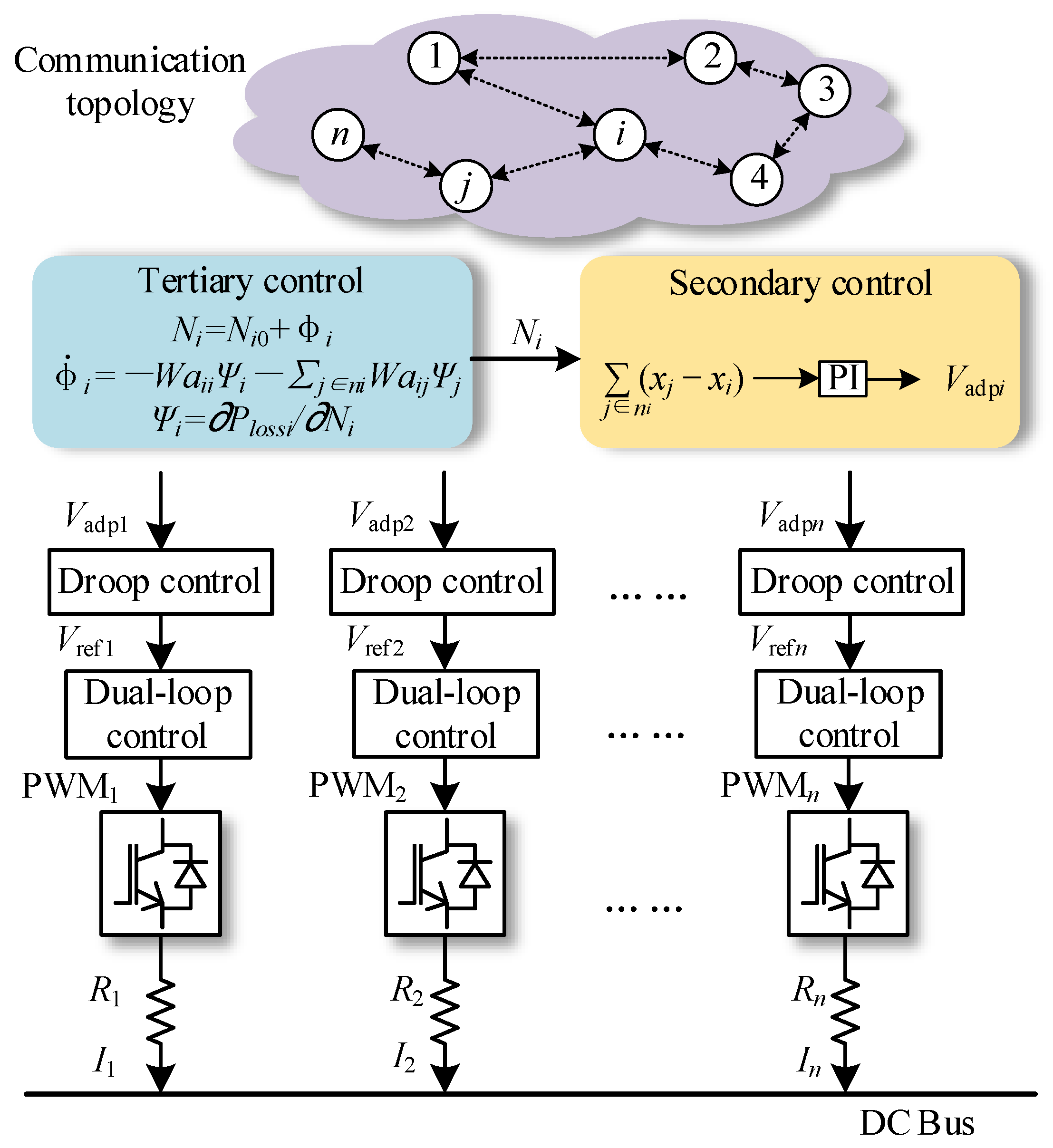
3. Hierarchical Control Design

3.1. DICOA

Based on the convex optimization theory, it is easily concluded that the unique minimum loss exists regardless of other factors. Now, it is assumed to be

$$P_{\mathrm{l}\mathrm{o}\mathrm{s}\mathrm{s}}^{*}=\inf \{\sum {\mathbf{P}}_{\mathbf{l}\mathbf{o}\mathbf{s}\mathbf{s}}=P_{\mathrm{tloss}}\left|{\mathbf{I}}^T\mathbf{N}=1\right.\}$$

(10)

where $\mathbf{N}={\left[N_1,N_2,\cdots N_n\right]}^T$, $\mathbf{I}={\left[\mathrm{1,1},\cdots 1\right]}^T$, $\sum {\mathbf{P}}_{\mathbf{l}\mathbf{o}\mathbf{s}\mathbf{s}}$ is the sum of the following vector:

$${\mathbf{P}}_{\mathrm{loss}}={\left[P_{\mathrm{loss}1},P_{\mathrm{loss}2},\cdots ,P_{\mathrm{loss}i},\cdots ,P_{\mathrm{loss}n}\right]}^T$$

(11)

Lemma 1.

Under assumption, ${\mathit{N}}^{*}={\left[N_1^{*},N_2^{*},\cdots N_n^{*}\right]}^T$is the optimal solution of objective function (9), if and only if ${\mathit{N}}^{*}$ satisfies

$$\begin{array}{c}\nabla {\mathit{P}}_{\mathrm{loss}}\left({\mathit{N}}^{*}\right)=-{\lambda }^{*}\mathit{I}\\ {\mathit{I}}^T{\mathit{N}}^{*}=1\end{array}$$

(12)

where $\nabla {\mathbf{P}}_{\mathrm{loss}}={\left[P_{\mathrm{loss}1}^{\prime }\left(N_1\right),P_{\mathrm{loss}2}^{\prime }\left(N_2\right),\cdots ,P_{\mathrm{loss}i}^{\prime }\left(N_i\right),\cdots ,P_{\mathrm{loss}n}^{\prime }\left(N_n\right)\right]}^T$ is the vector of gradients, and $\lambda$^* is the Lagrange multiplier of the optimal condition.

Proof. 

The Lagrange dual function of the proposed objective function is given as □

$$\begin{gathered} L\left(N_i,\lambda \right)=P_{\mathrm{tloss}}\left(N_i\right)+\lambda \ast g\left(N_i\right) \\ =\sum _{i=1}^n\left[\right(a_i+R_i\left)\right(N_i{I}_{\mathrm{tol}}{)}^2+b_i\left|N_i{I}_{\mathrm{tol}}\right|+c_i]+\lambda ({\sum }_{i=1}^n{N}_i-1) \end{gathered}$$

(13)

According to the Karush–Kuhn–Tucker optimization equations [17], the values in N^∗ are the optimal current-sharing coefficients if and only if the following two conditions can be satisfied:

$$\begin{array}{c}{P}_{\mathrm{loss}\mathrm{i}}^{\prime }\left(N_i\right)+{\lambda }^{*}=0\\ {\mathbf{I}}^T{\mathbf{N}}^{*}=1\end{array}$$

(14)

As shown in (12), under the optimal condition, the derivative of each loss function should be equal to $-{\lambda }^{*}$. Meanwhile, the second condition means the current-sharing coefficients should satisfy the supply–demand balance. Moreover, the conditions in (14) and (12) are equivalent to each other, which means the proof is completed.

As shown in Lemma 1, it can be concluded that $\nabla {\mathbf{P}}_{\mathrm{loss}}={\left[P_{\mathrm{loss}1}^{\prime }\left(N_1\right),P_{\mathrm{loss}2}^{\prime }\left(N_2\right),\cdots ,P_{\mathrm{loss}i}^{\prime }\left(N_i\right),\cdots ,P_{\mathrm{loss}n}^{\prime }\left(N_n\right)\right]}^T$ (also named incremental costs [25]) are identical under the optimal condition. Intuitively, the distribution loss optimization can be achieved by using consensus control for the loss gradients. Moreover, multi-step iteration is necessary because the global data cannot be acquired under a distributed control structure. After analysis, the following iteration optimization method (DICOA) is proposed to find the optimal current-sharing coefficients:

$$\left\{\begin{array}{c}{N}_i=N_{i0}+{\Phi }_i\\ {\dot{\Phi }}_i=-W{a}_{ii}{\Psi }_i-{\sum }_{j\in n_i}W{a}_{ij}{\Psi }_j\\ {\Psi }_i=\frac{\partial P_{\mathrm{l}\mathrm{o}\mathrm{s}\mathrm{s}i}}{\partial N_i}\end{array}\right.$$

(15)

where $N_{i0}$ is the initial value of $N_i$, and ${\sum }_{i=1}^n{N}_{i0}=1$; W is a constant, which affects the convergence speed; ${\Phi }_i$ is an intermediate variable. As shown in (9)–(15), the loss model and proposed DICOA are applicable for a general DC microgrid regardless of the number of distributed energy resources (DERs) or system topology.

Lemma 2.

By using DICOA, the current-sharing coefficients $N$ will converge to $N^{*}$.

Proof. 

As shown in (15), the iterative feedback term of each DER is the difference between its own incremental cost and that of its neighboring DERs. Thus, the variation in the local current- sharing coefficient at each step is described by a weighted sum of the differences between its local gradient value and those of the neighboring nodes. The proposed DICOA can be illustrated as follows: during the iteration process, the output current from nodes with higher marginal loss will be reduced while the output current from nodes with lower marginal loss will be reduced. In other words, by making trade-offs of the incremental cost, the incremental cost of all DERs will tend to be equal. After iterations, equations (12) and (14) can be satisfied, while the extremum point of the objective function can be found. □

To satisfy the equality constraint, the graph of the communication topology should be balanced, and the elements in the Laplacian matrix satisfy the following equation:

$$a_{ii}=-{\sum }_{j\in n_i}{a}_{ij}$$

(16)

During the whole updating process, the sum of the current-sharing coefficients satisfies the following conditions:

$${\sum }_{i=1}^n{N}_i={\sum }_{i=1}^n{N}_{i0}+{\sum }_{i=1}^n{\Phi }_i=1+{\sum }_{i=1}^n{\Phi }_i$$

(17)

By adding intermediate variables, the following is obtained:

$$\begin{gathered} {\sum }_{i=1}^n\left(-W{a}_{ii}{\Psi }_i-{\sum }_{j\in n_i}W{a}_{ij}{\Psi }_j\right)=-W{\sum }_{i=1}^n{a}_{ii}{\Psi }_i-W{\sum }_{i=1}^n{\sum }_{j\in n_i}{a}_{ij}{\Psi }_j \\ =W{\sum }_{i=1}^n{\sum }_{j\in n_i}{a}_{ij}{\Psi }_i-W{\sum }_{i=1}^n{\sum }_{j\in n_i}{a}_{ij}{\Psi }_{j}0 \end{gathered}$$

(18)

Obviously, in each iteration period, the sum of current-sharing coefficients ${\sum }_{i=1}^n{\Phi }_i$ = 1, which means the second equations in (12) and (14) can be satisfied. Therefore, the updated current-sharing coefficients satisfy the equality constraint during the optimization process. By considering the power constraint, the saturation link can be added as given by

$$N_i(k+1)=\left\{\begin{array}{cc}\frac{\left|I_{\mathrm{m}\mathrm{i}\mathrm{n}i}\right|}{\left|I_{\mathrm{t}\mathrm{o}\mathrm{l}}\left(k\right)\right|}& P_i<P_{\min i}\\ \frac{\left|I_{\mathrm{m}\mathrm{a}\mathrm{x}i}\right|}{\left|I_{\mathrm{t}\mathrm{o}\mathrm{l}}\left(k\right)\right|}& P_i>P_{\max i}\\ \left(15\right)& P_{\min i}\le P_i\le P_{\max i}\end{array}\right.$$

(19)

where I_mini and I_maxi are the minimum value and maximum value of the injection currents. Obviously, the loss model is also a concave function irrespective of the power clip or number of power supplies [15].

Specifically, we use addition and subtraction iteration or the dual variables. For comparison, two methods, i.e., Lagrange multiplier [14] and dual ascent algorithm [2], are presented here. The performance indexes of the three methods are summarized in

Table 1. Summarization of Key Performance Indexes.

Algorithms/Methods	Division	Iteration
Lagrange Multiplier method	✓	✕
Dual ascent algorithm	✓	✓
DICOA	✕	✓

. The division is avoided by the proposed DICOA, which mitigates the computational burden on microprocessors. By using distributed iterations, the scalability of DICOA is enhanced for large-scale DC microgrids.

3.2. Lower Control Layers

In this paper, the regulations of the current-sharing errors are implemented by a cascaded control: the adaptive output voltage term V_adpi for distributed secondary control is used to regulate the output voltage reference V_refi, a dual-loop control to regulate the duty ratio.

(1)

With the use of the optimal current distribution coefficients derived by the DICOA, the current sharing error of the i-th DER can be calculated by

$$e_i={\sum }_{j\in n_i}(x_j-x_i)$$

(20)

where $x_i=I_i/N_i^{*}$ is a control variable. The current sharing errors, required to be regulated at zero, yield

$$\frac{I_1}{N_1^{*}}=\frac{I_2}{N_2^{*}}=\cdots =\frac{I_n}{N_n^{*}}$$

(21)

For the distributed secondary control, the PI controllers are adopted as

$$V_{\mathrm{a}\mathrm{d}\mathrm{p}i}=(k_{\mathrm{P}i}+\frac{k_{\mathrm{I}i}}{s})e_i$$

(22)

where k_Pi and k_Ii are gains.

(2)

In the droop control part, the output voltage reference can be calculated as

$$V_{\mathrm{r}\mathrm{e}\mathrm{f}i}=V_{\mathrm{nom}}-R_{\mathrm{d}i}{I}_i+V_{\mathrm{a}\mathrm{d}\mathrm{p}i}$$

(23)

where V_nom is the nominal value of the bus voltage, and R_di is the pre-given virtual resistance. Moreover, a saturation limiter can be used to regulate the voltage within the tolerances. In this way, only the inequality constraint of the injected power is considered in the DICOA.

(3)

For the voltage–current control, both the DC source current and the duty ratio are required to be regulated within the tolerances.

By taking the Laplace transformation of (23), the adaptive voltage is written as

$$s{\mathbf{V}}_{\mathbf{a}\mathbf{d}\mathbf{p}}\left(s\right)=s{\mathbf{k}}_{\mathbf{p}}\mathcal{L}\left\{\mathbf{x}\left(s\right)\right\}+{\mathbf{k}}_{\mathbf{I}}\mathcal{L}\left\{\mathbf{x}\left(s\right)\right\}=\mathbf{G}\left(s\right)\mathcal{L}\left\{\mathbf{x}\left(s\right)\right\}$$

(24)

where ${\mathbf{V}}_{\mathbf{a}\mathbf{d}\mathbf{p}}\left(s\right)={\left[V_{\mathrm{a}\mathrm{d}\mathrm{p}1}\left(s\right),V_{\mathrm{a}\mathrm{d}\mathrm{p}2}\left(s\right),\cdots V_{\mathrm{a}\mathrm{d}\mathrm{p}n}\left(s\right)\right]}^T$; $\mathbf{x}\left(s\right)=\left[x_1\right(s),x_2(s),\dots ,x_n(s){]}^T$; ${\mathbf{k}}_{\mathbf{P}}=\mathrm{diag}\left(k_{P1},k_{P2},\dots ,k_{Pn}\right)$, ${\mathbf{k}}_{\mathbf{I}}=\mathrm{diag}\left(k_{I1},k_{I2},\dots ,k_{In}\right)$; and $\mathbf{G}\left(s\right)=\mathrm{diag}\left(s{k}_{P1}+k_{I1},s{k}_{P2}+k_{I2},...,s{k}_{Pn}+k_{In}\right)$. At steady state (i.e., $t\to \mathrm{\infty }$), using final value theorem,

$$\underset{s\to 0}{\lim }s\mathcal{L}\left\{\mathbf{x}\left(s\right)\right\}=0$$

(25)

As analyzed above, the control variables will be converged to consensus. In practice, the communication delay in the control process will affect the control performance and the system stability [17]. For the proposed hierarchical control, the sampling frequency of the lower control layer is much faster than that of the higher control layer. By considering the inertia of converters, the updating period of DICOA is much longer than the control period of secondary control. Therefore, the system stability can be guaranteed with the considerations of communication delay. The multi-layer control diagram is presented in Figure 2.

4. Simulation Results

For the simulation case studies, a six DER-based DC microgrid is built for verification. The main specifications of the DERs and electric network are given in

Table 2. Main Specifications of the DERs in the Simulation.

Descriptions	Symbol	Value
Nominal DC bus voltage	Vnom	48 V
Lower limit of the DC bus voltage	Vmin	45.6 V
Upper limit of the DC bus voltage	Vmax	50.4 V
Lower output power limit of the DERs	Pmin	0 W
Upper output power limit of the DERs	Pmax	350 W
Source voltage of the DERs	VSi	24 V
Inductances of the converters	Li	460 μH
Output capacitances of the converters	Ci	10.1 μF
Line resistance of the DER1	R1	0.53 Ω
Line resistance of the DER2	R2	1.18 Ω
Line resistance of the DER3	R3	0.16 Ω
Line resistance of the DER4	R4	0.64 Ω
Line resistance of the DER5	R5	0.46 Ω
Line resistance of the DER6	R6	0.67 Ω
Communication delay	τ	0.01 s

and

Table 3. Parameters of Controllers in the Simulation.

Descriptions	Symbol	Value
Mutual weights	Wij	0.0002
Virtual resistances	Rdi	0.05 Ω
Conversion loss coefficients of DER1	α	1.161
	β	0.730
	γ	1.693
Conversion loss coefficients of DER2	α	0.641
	β	0.547
	γ	5.260
Conversion loss coefficients of DER3	α	1.693
	β	5.260
	γ	3.540
Conversion loss coefficients of DER4	α	0.730
	β	1.620
	γ	2.800
Conversion loss coefficients of DER5	α	1.939
	β	1.830
	γ	2.693
Conversion loss coefficients of DER6	α	0.917
	β	1.847
	γ	3.260
Switching frequency of the converters	fs	100 kHz
Updating frequency of the DICOA	f3	0.2 Hz
Sampling frequency of the distributed secondary control	f2	1 kHz
Sampling frequency of the local control	f1	100 kHz

, respectively. In the simulations, the parameters of the mutual-weights, PI controllers, converters, and virtual resistances are identical for all DERs. The limitations of bus voltage and the output power are also given in the table. As an important parameter, the value of mutual weight (selected as 0.0002 in simulations) determines the dynamic performance of DICOA. Four different cases are studied, i.e., the normal operation for Case 1, power clip for Case 2, communication failure for Case 3, and plug-out of one DER for Case 4. Meanwhile, the different communication topologies of cases are given in Figure 3.

For the proposed six DER-based DC microgrid, the concave property of the distributed loss function with six variables (current distribution coefficients) has been theoretically proofed in Section 2. Furthermore, by the fitting value method, the loss models can be presented as curved surfaces. In Figure 4, the load current sink is 20 A, and three current distribution coefficients are selected and fixed at 0.1 (i.e., N₄ = N₅ = N₆ = 0.1 for Figure 4a, N₅ = N₆= N₁ = 0.1 for Figure 4b, N₆ = N₁ = N₂ = 0.1 for Figure 4c, N₁ = N₂ = N₃ = 0.1 for Figure 4d, N₂ = N₃ = N₄ = 0.1 for Figure 4e, and N₃ = N₄ = N₅ = 0.1 for Figure 4f). In this way, six loss functions with three variables and one equality constraint can be drawn as 3D concave surfaces. Apparently, all surfaces are concave, and the minimum power loss is 198.3 W, 183.4 W, 192.7 W, 181.2 W, 193.9 W, and 184.6 W. Therefore, the proposed distribution loss model is verified to be convex w.r.t. current-sharing coefficients.

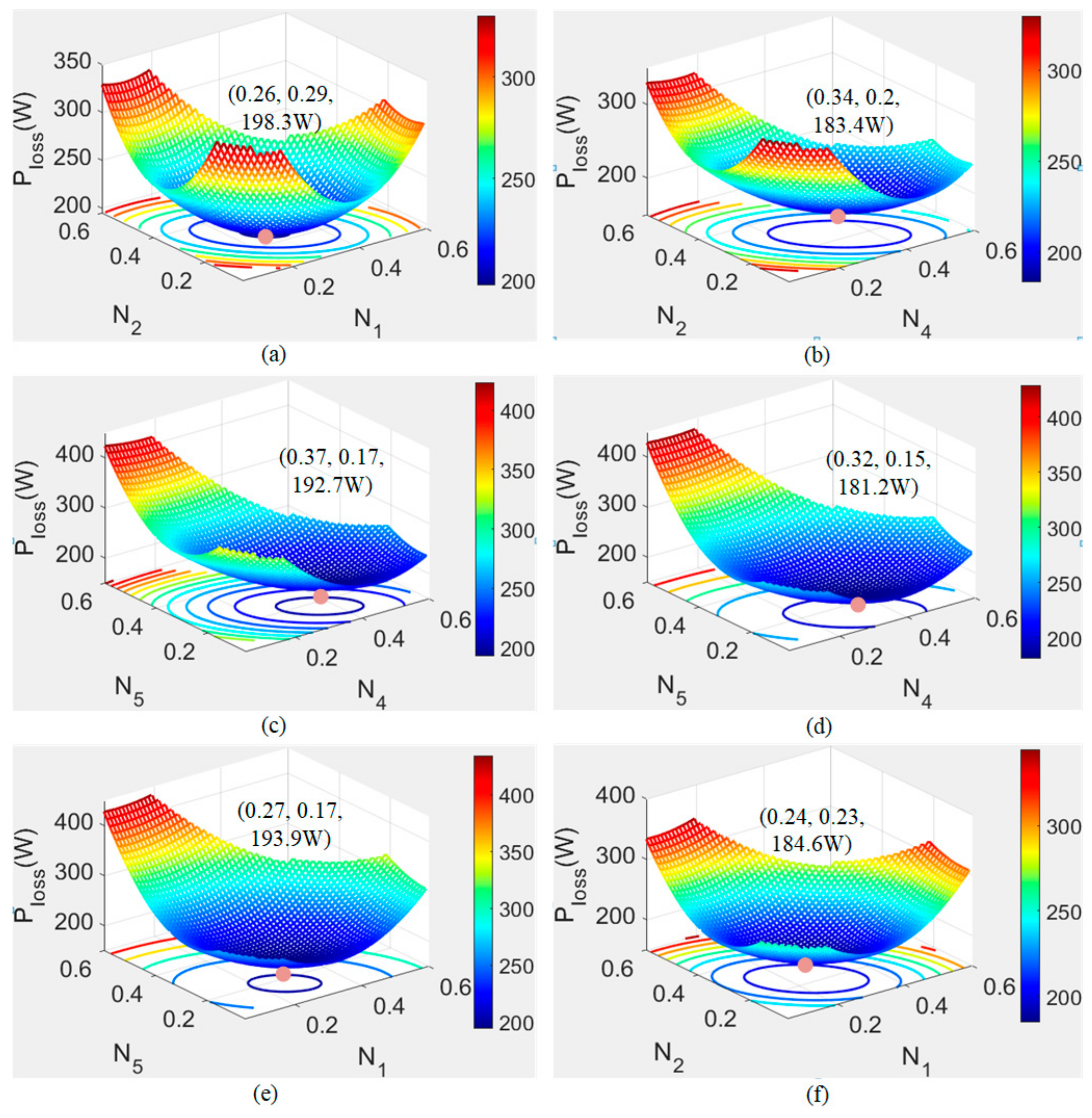
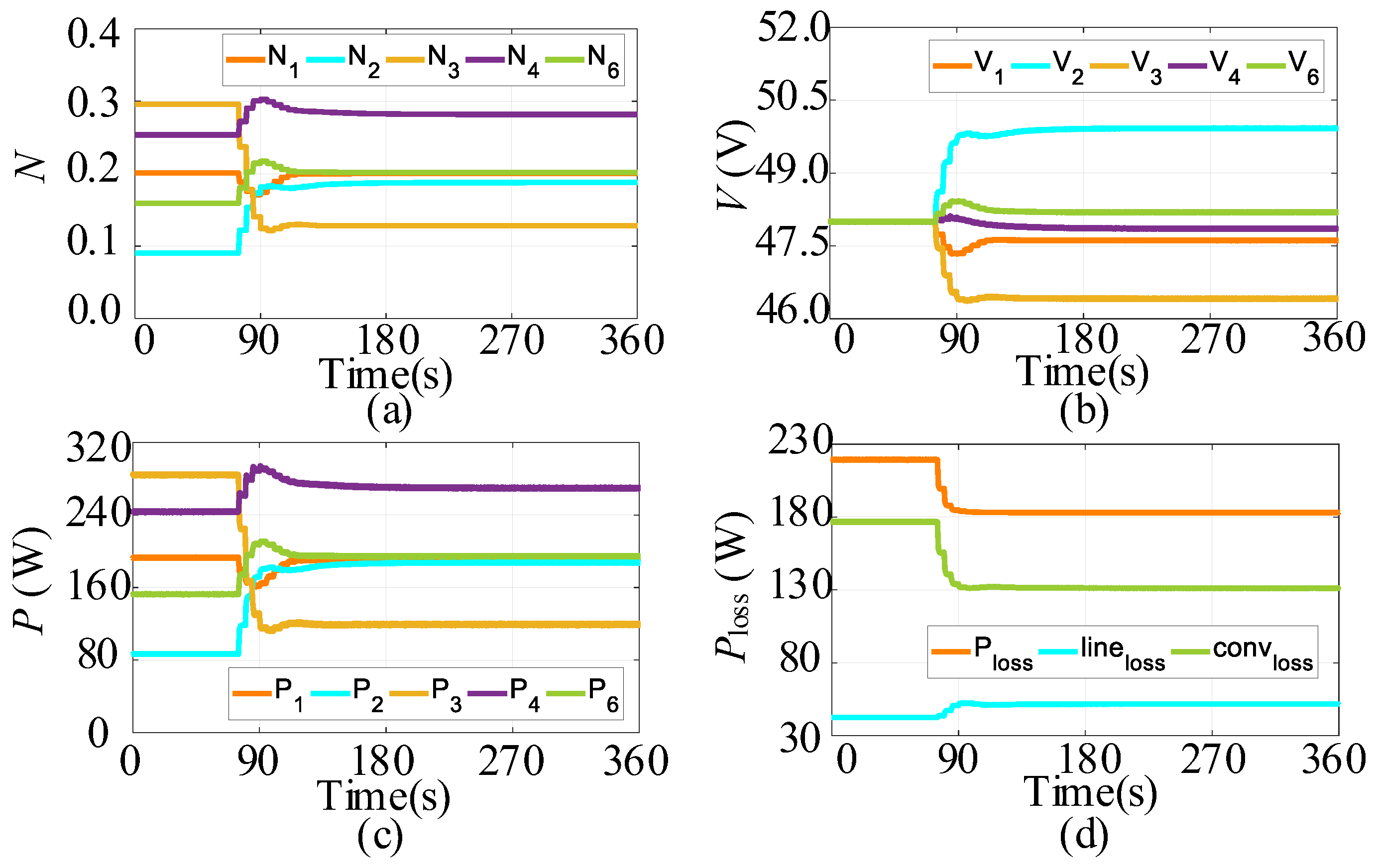
• Case 1: System Operation of the DC Electric Network Based on Six DERs

Under the load current of 20 A, the DC electric network based on the six DERs operates for a period of 300 s. Meanwhile, the wire loss optimization strategy in [3,16] is adopted at 0 s for comparison. As shown in Figure 5, the output currents in the DC microgrid are dispatched according to the wire loss minimization-based current ratio. At steady-state, the converter loss, wire loss, and the total loss are regulated to be 164.8 W, 34.6 W, and 199.4 W, respectively. From 75 s, the current-sharing coefficients are updated by the proposed DICOA in which the iteration cycle is 5 s. Afterwards, the optimal coefficients by DICOA are $N_1^{*}=0.178$, $N_2^{*}=0.167$, $N_3^{*}=0.110$, $N_4^{*}=0.249$, $N_5^{*}=0.118$, and $N_6^{*}=0.178$. At each iteration, by adjusting the voltages, the current dispatching is achieved by the secondary control. At new steady states, the total loss is reduced to 167.9 W. Compared with that of the conventional method, the total loss of the DC electric network is reduced by 31.5 W, which is about 15.8%.

• Case 2: Output Power Limitation

In the second case, the load current is increased to 35 A and the line resistances are varied to be R₁ = 0.53 Ω, R₂ = 1.18 Ω, R₃ = 0.36 Ω, R₄ = 0.32 Ω, R₅ = 0.46 Ω, and R₆ = 0.67 Ω. In Figure 6, the wire loss optimization control, DICOA without constraint, and complete control strategy are used in the DC network from 0 s to 50 s, 50 s to 160 s, and 160 s to 300 s, respectively. By using the current distribution coefficients by wire loss optimization, the generated loss of the DC microgrid is 490.6 W before 50 s. With the use of convex optimization, the optimized value of N₄ is 0.247 without considering the power constraint. However, the power from DER4 is 413 W in the period of 50 s to 160 s. Therefore, the in-equality constraint should be added in the hierarchical control strategy. At 160 s, the power from DER4 is limited at 350 W (upper bound), as shown in Figure 6c. When the N₄ is fixed at 0.215, based on the new convex model, the proposed DICOA continuously updates the remaining five current distribution coefficients. At the new steady state, the power distribution coefficients of the four DERs are updated to be $N_1^{*}=0.188$, $N_2^{*}=0.177$, $N_3^{*}=0.110$, $N_4^{*}=0.215$, $N_5^{*}=0.123$, and $N_6^{*}=0.187$. Additionally, the bus voltages of the DC electric network are always regulated within the limitations, as shown in Figure 6b. Due to the power inequality constraint, the new optimal point deviates from the ideal minimum point, and the resulting loss is higher than the loss at 160 s. However, with the use of the proposed DICOA, the total loss is still reduced by 65.3 W, in which the power loss saving is about 13.3%.

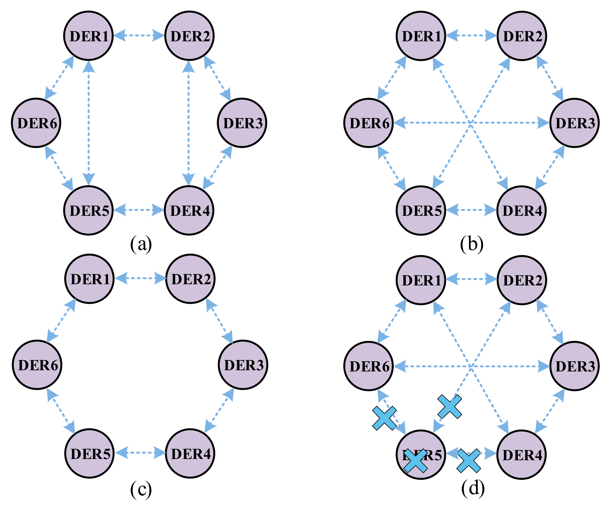
• Case 3: Communication Failure

In Case 3, the communication links between DER1 and DER5 and between DER2 and DER4 are cut off as shown in Figure 3, while the remaining structure and parameters are the same as those in Case 1. In Figure 7, the conventional wire loss optimization control and proposed control are implemented from 0 s to 140 s and from 140 s to 560 s, respectively. By using the same parameters, the control results based on the conventional method are same as those in Case 1, i.e., the distribution loss is 199.4 W. From 140 s, the current distribution coefficients are updated by the proposed DICOA in a cycle of 5 s. At steady state, the current coefficients updated by DICOA are $N_1^{*}=0.178$, $N_2^{*}=0.167$, $N_3^{*}=0.110$, $N_4^{*}=0.249$, $N_5^{*}=0.118$, and $N_6^{*}=0.178$, which are exactly the same as the ones being optimized in Case 1. As compared with the results in Figure 5, the only difference is that the iteration rate in Figure 8 is slower with fewer communication links. The total loss by the designed strategy is reduced by about 15.8% (from 199.4 W to 167.9 W). It is also identical to the loss reduction in Case 1. This case indicates that the global convex optimization can be realized by DICOA only if the graph of the data-exchanging network has connectivity.

• Case 4: Plug-Out of One DER

In the last simulation case, DER5 is removed from the DC electric network, and the communication topology is shown in Figure 3d. Thereby, the graph of new communication topology (with five DERs) is still a spinning tree. The current sink is set to be 20 A, and the system operation time is 360 s. In Figure 8, the conventional wire loss optimization strategy is applied before 75 s, and the proposed DICOA is implemented after 75 s. By adopting the DICOA, the current-sharing coefficients are calculated to be $N_1^{*}=0.2$, $N_2^{*}=0.188$, $N_3^{*}=0.128$, $N_4^{*}=0.282,$ and $N_6^{*}=0.202$ at steady-state. The total loss is reduced from 219.3 W to 183.1 W (by about 16.5%). Regardless of the number of DERs and communication structure, the scalability of the proposed DICOA-based multi-layer control is verified.

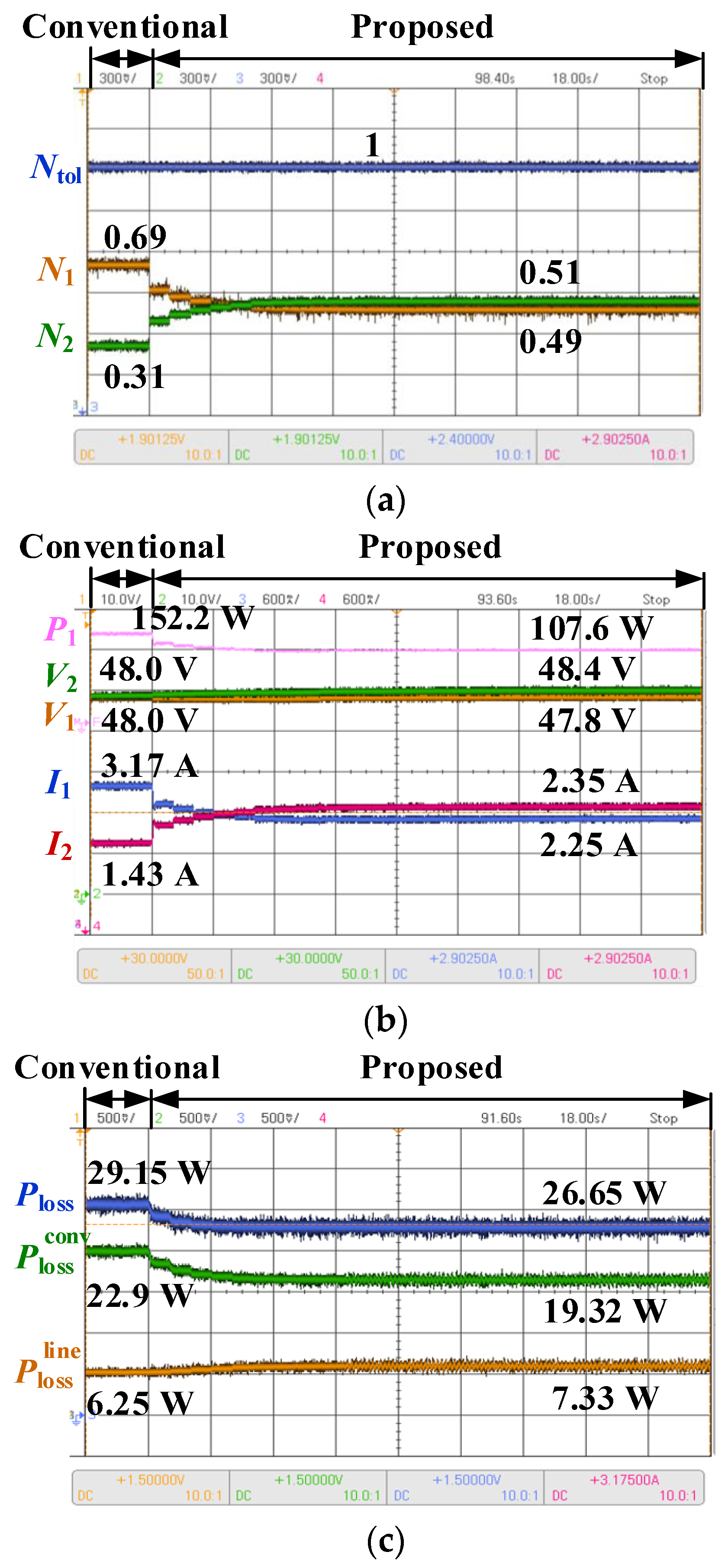
5. Experimental Results

In experiments, the boost converter-based DERs are adopted to construct the DC microgrid. In details, two experimental scenarios are carried out. The data of DERs are exchanged among them. The virtual resistances, operation frequency, and the sampling period of the secondary control are the same as the ones in Table 3. The line resistances and PI controllers of secondary control are given in

Table 4. Parameters in Experiments.

Scenarios	Line Resistances		PI Compensators
	R1 (Ω)	R2 (Ω)	KPi	KIi	KP1i	KI1i	KP2i	KI2i
1	0.43	0.94	0.2	1.0	0.025	0.1	0.05	0.1
2	0.2	0.2	0.2	1.0	0.025	0.1	0.05	0.1

. After analysis, the mutual weights are set to 0.002. The updating frequency of the DICOA is set to 1/6 Hz. The loss coefficients are obtained as follows: α₁ = 1.161, β₁ = 0.730, and γ₁ = 1.693 for DER1, α₂ = 0.641, β₂ = 0.547, and γ₂ = 5.260 for DER2, and α₃ = 1.693, β₃ = 5.26, and γ₃ = 3.54 for DER3. In this way, the concave property is further proofed by the experiment. In experiments, the intermediate variables (current-sharing coefficients and power loss) are outputted by pins of DSP, while the remaining variables are measured by probes.

• Scenario 1: Normal Operation

Under the load current of 4.6 A, the experimental waveforms under the proposed hierarchical control strategy are presented in Figure 9. From 0 s to 18 s, the current ratio N₁: N₂ = 0.69: 0.31, obtained by the conventional method, is used for current sharing. At steady state, the variables of the two DERs are regulated to be I₁ = 3.17 A, V₁ = 48.0 V and I₂ = 1.43 A, V₂ = 48.0 V, with output power values of 152.2 W and 68.6 W, respectively. Under the wire loss optimization method, the total loss, wire loss, and converter loss are 29.15 W, 6.25 W, and 22.9 W, respectively. By updating in the period of 6 s, the current dispatching coefficients are converged with the optimal values with the help of DICOA. Afterwards, the optimal coefficients are updated to be $N_1^{*}=0.49$ and $N_2^{*}=0.51$. With the help of secondary control, the currents, and voltages of DERs are 2.25 A, 47.8 V and 2.35 A, 48.4 V, with output power values of 107.6 W and 113.7 W. Finally, the total loss of the DC electric network is optimized to be 26.65 W, which is reduced by 8.58%.

• Scenario 2: Injection Power Limitation

In the second experimental scenario, the experimental waveforms in the period from 0 s to 120 s under a 5.2 A load are presented in Figure 10. Before 12 s, the current ratio based on the conventional method, N₁:N₂ = 0.38:0.62, is used for distributed current sharing (1.98 A and 3.22 A). Subsequently, the total loss by the wire loss optimization method is 36.5 W. When the DICOA is activated at 12 s, the current distribution coefficients start the iteration, and they are optimized as $N_1^{*}=0.22$ and $N_2^{*}=0.78$ at steady state. Meanwhile, the variables of the two DERs are I₁ = 1.14 A, V₁ = 47.9 V and I₂ = 4.06 A, V₂ = 49.8 V. Without considering the power limitation, the optimal current distribution coefficients based on conventional optimization will converge to $N_1^{*}=0.12$ and $N_2^{*}=0.88$. By using DICOA, the injection power from DER2 is limited at the pre-defined maximum value. Finally, the total loss based on the proposed DICOA is reduced to 32.2 W. Compared to the wire loss optimization control, the loss reduction of the DC microgrid is 11.8%. Thus, the results of Scenario II verify that the proposed hierarchical control can reduce loss even if the output power is clipped at the boundaries.

6. Conclusions

In this paper, a general distribution loss model with generality for various DC distribution systems and conditions is proposed. Both converter loss and line loss are included in the proposed distribution loss model. Then, distribution loss is described by the function of the current allocation coefficients of DERs. With convexity, the global minimization of the distribution loss can be achieved by adjusting the current allocation coefficients. Then, a distributed loss optimization algorithm, DICOA, is designed to find the optimal current-sharing coefficients. By considering the characteristics of the power electronic system, a hierarchical control strategy based on multiple time scales is designed to realize the loss optimization objective. The comprehensive results of various case studies are presented to verify the proposed control strategy for loss reduction. In view of some application limitations, more modelling and optimization work for the DC microgrid will be presented in future work.

References

1. Babazadeh-Dizaji, R.; Hamzeh, M. Distributed hierarchical control for optimal power dispatch in multiple DC microgrids. IEEE Syst. J. 2020, 14, 1015–1023. [Google Scholar] [CrossRef]
2. Jiang, Y.; Yang, Y.; Tan, S.C.; Hui, S.Y.R. Dual-ascent hierarchical control-based distribution power loss reduction of parallel-connected distributed energy storage systems in dc microgrids. IEEE J. Emer. Sel. Top. Ind. Electron. 2023, 4, 137–146. [Google Scholar] [CrossRef]
3. Yang, Y.; Tan, S.C.; Hui, S.Y.R. Mitigating distribution power loss of DC microgrids with DC electric springs. IEEE Trans. Smart Grid 2018, 9, 5897–5906. [Google Scholar] [CrossRef]
4. Pires, V.F.; Pires, A.; Cordeiro, A. DC Microgrids: Benefits, Architectures, Perspectives and Challenges. Energies 2023, 16, 1217. [Google Scholar] [CrossRef]
5. Su, W.; Yun, S.; Li, H.; Lu, H.H.C.; Fernando, T. An MPC-based dual-solver optimization method for DC microgrids with simultaneous consideration of operation cost and power loss. IEEE Trans. Power Syst. 2021, 36, 936–947. [Google Scholar] [CrossRef]
6. Fan, Z.; Fan, B.; Peng, J.; Liu, W. Operation loss minimization targeted distributed optimal control of DC microgrids. IEEE Syst. J. Early Access 2021, 15, 5186–5196. [Google Scholar] [CrossRef]
7. Ren, Y.; Xu, M.; Zhou, J.; Lee, F.C. Analytical loss model of power MOSFET. IEEE Trans. Power Electron. 2006, 21, 310–319. [Google Scholar]
8. Rodríguez, M.; Rodríguez, A.; Miaja, P.F.; Lamar, D.G.; Zúniga, J.S. An insight into the switching process of power MOSFETs: An improved analytical losses model. IEEE Trans. Power Electron. 2010, 25, 1626–1640. [Google Scholar] [CrossRef]
9. Yuan, W.; Wang, Y.; Liu, D.; Deng, F.; Chen, Z. Efficiency-prioritized droop control strategy of AC microgrid. IEEE J. Emerg. Sel. Top. Power Electron. 2020, 3, 2936–2950. [Google Scholar] [CrossRef]
10. Wang, H.; Khambadkone, A.M.; Yu, X. Control of parallel connected power converters for low voltage microgrid-part II: Dynamic electrothermal modeling. IEEE Trans. Power Electron. 2010, 25, 2971–2980. [Google Scholar] [CrossRef]
11. Wang, Y.; Chen, D.L.Z.; Liu, P. A hierarchical control strategy of microgrids toward reliability enhancement. In Proceedings of the International Conference on Smart Grid (icSmartGrid), Nagasaki, Japan, 4–6 December 2018; pp. 123–128. [Google Scholar]
12. Bartal, P.; Nagy, I. Game theoretic approach for achieving optimum overall efficiency in DC/DC converters. IEEE Trans. Ind. Electron. 2014, 61, 3202–3209. [Google Scholar] [CrossRef]
13. Jiang, Y.; Yang, Y.; Tan, S.C.; Hui, S.Y.R. Power loss minimization of parallel-connected DERs in dc microgrids using a distributed hierarchical control. IEEE Trans. Smart Grid 2022, 13, 4538–4550. [Google Scholar] [CrossRef]
14. Jiang, Y.; Yang, Y.; Tan, S.C.; Hui, S.Y.R. Distribution power loss mitigation of parallel-connected distributed energy resources in low-voltage DC microgrids using a Lagrange multiplier-based adaptive droop control. IEEE Trans. Power Electron. 2021, 36, 9105–9118. [Google Scholar] [CrossRef]
15. Shi, M.; Chen, X.; Zhou, J.; Chen, Y.; Wen, J.; He, H. Advanced secondary voltage recovery control for multiple HESSs in a droop-controlled DC microgrid. IEEE Trans. Smart Grid 2019, 10, 3828–3839. [Google Scholar] [CrossRef]
16. Cevher, V.; Becker, S.; Schmidt, M. Convex optimization for big data: Scalable, randomized, and parallel algorithms for big data analytics. IEEE Signal Process. Mag. 2014, 31, 32–43. [Google Scholar] [CrossRef]
17. Boyd, S.; Vandenberghe, L. Convex Optimization; Cambridge University Press: Cambridge, UK, 2004. [Google Scholar]
18. Ali, S.; Zheng, Z.; Aillerie, M.; Sawicki, J.P.; Pera, M.C.; Hissel, D. A review of DC Microgrid energy management systems dedicated to residential applications. Energies 2021, 14, 4308. [Google Scholar] [CrossRef]
19. Meng, L.; Shafiee, Q.; Trecate, G.F.; Karimi, H.; Fulwani, D.; Lu, X.; Guerrero, J.M. Review on control of DC microgrids and multiple microgrid clusters. IEEE J. Emerg. Sel. Topics Power Electron. 2017, 5, 928–948. [Google Scholar]
20. Sahoo, S.; Mishra, S. A distributed finite-time secondary average voltage regulation and current sharing controller for DC microgrids. IEEE Trans. Smart Grid 2019, 10, 282–292. [Google Scholar] [CrossRef]
21. Nasirian, V.; Davoudi, A.; Lewis, F.L.; Guerrero, J.M. Distributed adaptive droop control for DC distribution systems. IEEE Trans. Energy Convers. 2014, 29, 944–956. [Google Scholar] [CrossRef]
22. Guo, F.; Wang, L.; Wen, C.; Zhang, D.; Xu, Q. Distributed voltage restoration and current sharing control in islanded DC microgrid systems without continuous communication. IEEE Trans. Ind. Electron. 2020, 67, 3043–3053. [Google Scholar] [CrossRef]
23. Xing, L.; Xu, Q.; Guo, F.; Wu, Z.G.; Liu, M. Distributed secondary control for DC microgrid with event-triggered signal transmissions. IEEE Trans. Sustain. Energy 2021, 12, 1801–1810. [Google Scholar] [CrossRef]
24. Poursafar, N.; Taghizadeh, S.; Hossain, M.J.; Guerrero, J.M. An optimized distributed cooperative control to improve the charging performance of battery energy storage in a multiphotovoltaic islanded DC microgrid. IEEE Syst. J. 2022, 16, 1170–1181. [Google Scholar] [CrossRef]
25. Xiao, L.; Boyd, S. Optimal scaling of a gradient method for distributed resource allocation. J. Optimiz. Theory Appl. 2006, 29, 469–488. [Google Scholar] [CrossRef]
Figure 1. A general DC microgrid with parallel-connected DERs, (a) simplified architecture, and (b) simplified circuit diagram.
Energies 16 08106 g001
Figure 2. Control diagram of the hierarchical control strategy.
Energies 16 08106 g002
Figure 3. Communication network in simulations, (a) Case1, (b) Case2, (c) Case3, and (d) Case4.
Energies 16 08106 g003
Figure 4. Loss surfaces versus current distribution coefficients of the DC microgrid, (a) N4 = N5 = N6 = 0.1, (b) N1 = N5 = N6 = 0.1, (c) N1 = N2 = N6 = 0.1, (d) N1 = N2 = N3 = 0.1, (e) N2 = N3 = N4 = 0.1, (f) N4 = N5 = N3 = 0.1.
Energies 16 08106 g004
Figure 5. Simulation results of Case 1, (a) current-sharing coefficient, (b) voltage, (c) power, and (d) loss.
Energies 16 08106 g005
Figure 6. Simulation results of Case 2, (a) current-sharing coefficient, (b) voltage, (c) power, and (d) loss.
Energies 16 08106 g006
Figure 7. Simulation results of Case 3, (a) current-sharing coefficient, (b) voltage, (c) power, and (d) loss.
Energies 16 08106 g007
Figure 8. Simulation results of Case 4, (a) current-sharing coefficient, (b) voltage, (c) power, and (d) loss.
Energies 16 08106 g008
Figure 9. Experimental results of Scenario 1, (a) current-sharing coefficient, (b) voltage, current, power, and (c) loss.
Energies 16 08106 g009
Figure 10. Experimental results of Scenario 2, (a) current-sharing coefficient, (b) voltage, current, power, and (c) loss.
Energies 16 08106 g010