Abstract
Deep comprehension of wind farm performance is a complicated task due to the multivariate dependence of wind turbine power on environmental variables and working parameters and to the intrinsic limitations in the quality of SCADA-collected measurements. Given this, the objective of this study is to propose an integrated approach based on SCADA data and Computational Fluid Dynamics simulations, which is aimed at wind farm performance analysis. The selected test case is a wind farm situated in southern Italy, where two wind turbines had an apparent underperformance. The concept of a space–time comparison at the wind farm level is leveraged by analyzing the operation curves of the wind turbines and by comparing the simulated average wind field against the measured one, where each wind turbine is treated like a virtual meteorological mast. The employed formulation for the CFD simulations is Reynolds-Average Navier–Stokes (RANS). In this work, it is shown that, based on the above approach, it has been possible to identify an anemometer bias at a wind turbine, which has subsequently been fixed. The results of this work affirm that a deep comprehension of wind farm performance requires a non-trivial space–time comparison, of which CFD simulations can be a fundamental part.
1. Introduction
The comprehension of wind turbine performance in a real-world environment [1] is, in general, a complicated task. This occurs substantially for two reasons:
- the wind turbine power has a multivariate dependence on environmental factors, on working parameters, and on the health status of the machine;
- there are data quality issues related to the wind speed measurement.
As regards the latter point, the standard is that the wind speed at a wind turbine site is measured by cup- or ultrasonic anemometers, which are placed behind the rotor span, and the free stream wind speed is estimated ex post through a nacelle transfer function. Several environmental factors on which the power of a wind turbine depends are not measured in industrial plants, mainly for economic reasons. Some examples are the vertical components of the wind flow [2], the turbulence intensity [3], the humidity, the temperature [4], and so on. This means that in case the wind turbine is situated in a harsh environment [5] or is operating incorrectly (for example, if it is subjected to systematic yaw error [6,7]), the interaction between the wind field and the wind turbine rotor is different with respect to standard conditions and typically unpredictable. Furthermore, it is not rare that anemometers of industrial wind turbines are affected by bias [8,9,10] and therefore do not measure the wind speed correctly.
The most adopted method for wind turbine verification is the power curve analysis [11]. The power curve is simply the relationship between the input (wind speed) and the output (power) of a wind turbine. For the above-cited reasons, it is well established that the power curve of a wind turbine is site dependent [12], which means that the power curve of the same wind turbine model situated in different environments looks different. Given this, the design specifications of the power curve of a certain wind turbine model are useful only to a certain extent because there is no precise ground truth about how the measured power curve should appear at a given real-world site.
As regards the multivariate dependence of wind turbine power on operational parameters, a meaningful simplification is that the power that should be extracted by a wind turbine is given in Equation (1) [13]:
where R is the rotor diameter, is the air density, v is the free stream wind speed and is the power coefficient which depends on the blade pitch and on the rotor speed through the tip-speed ratio .
Given the above considerations and, most of all, the absence of a ground truth for performance verification, the most consistent approach is the space–time comparison [14], which is based on the assumption that the behavior of a wind turbine should be reasonably similar to itself over time and that the behavior of wind turbines of the same model at the same site should, as well, be reasonably similar. In a nutshell, the scientific objective of the present study is to pursue this concept further with respect to the state-of-the-art. The main innovative aspect of this work is that the two sources of complexity regarding wind turbine performance interpretation (which are the multivariate behavior and the wind speed data quality issues) are disentangled. This is achieved by separately employing SCADA data analysis methods [15] and Computational Fluid Dynamics (CFD) simulations and interpreting them jointly. The former method is applied to address the multivariate behavior of the power on the working parameters, and the latter to address the comprehension of the wind field on site and how it is measured by the wind turbines. The innovativeness does not regard every single method in particular, although it should be noted that the application of CFD simulations to a wind farm operational assessment is, in general, overlooked; rather, the approach regards the overall application and the interpretation. The study is organized as an academia–industry collaboration between the University of Perugia and the Fera company, and it is devoted to a real-world test-case study: a wind farm situated in Italy, composed of seven wind turbines having 3.4 MW of rated power each.
Two methods based on SCADA data are employed:
- The analysis of operation curves [16] which do not depend on the measurement of wind speed. The space–time comparison is pursued in order to individuate if there are differences in the wind turbines suspected of under-performance.
- The analysis of the power of the wind turbines of interest as a function of the power of nearby reference wind turbines. This method is typically called power–power or side–side and has been applied in the literature for evaluating small energy gains due to technology optimizations [17,18].
As anticipated above, the numerical method selected in this study consists of CFD simulations of the free wind flow over the wind farm. WindSim software has been employed for the solution of the Reynolds-Averaged formulation of the Navier–Stokes equations (RANS). The rationale for this analysis is that a possible anemometer bias at a wind turbine could be individuated in the form of a mismatch between the simulated wind field and the wind field measured by the nacelle anemometer of the wind turbine of interest. Once again, the space comparison between wind turbines from the same site comes in handy, and this is pursued in an original way. The hypothesis of anemometer bias is confirmed if the mismatch between the numerical simulations and measurements distinguishes the suspected wind turbine with respect to what happens for the rest of the fleet. From this point of view, each wind turbine can be conceptually considered a meteorological mast that can be employed for reference or validation.
Regarding the test case of this work, the above summarized holistic approach provided the solution to a measurement bias problem. Indeed, based upon the analyses reported in this work that were conducted, the nacelle anemometer of one wind turbine has been replaced, and the anomaly has been fixed.
2. The Test Case and the Data Set
The wind farm is composed of seven wind turbines having 3.4 MW of rated power each. The hub height is 96.5 m, and the rotor diameter is 104 m. The blade pitch angle is controlled electrically. The layout of the wind farm is reported in Figure 1. As can be deduced from the further information reported in Section 3, the wind farm is poorly affected by wakes, and the terrain is not particularly complex. Therefore, wind turbines are expected to perform similarly.
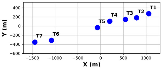
Figure 1.
The layout of the test case wind farm.
The nacelle anemometers of T2 and T4 have been replaced (the date is not reported for confidentiality). This allows for comparing the behavior before and after the replacement.
Data Pre-Processing
The data at our disposal go from 1 January 2016 to 31 October 2022. The available validated measurements have ten minutes of averaged time, and for each wind turbine are the following:
- Wind Speed v measured by the ultrasonic nacelle anemometer (m/s);
- Output power P (kW);
- Blade pitch angle ();
- Rotor speed (rpm);
- Gearbox speed (rpm).
Appropriate data pre-processing is fundamental in order to interpret the wind turbine performance correctly. In particular, a two-step method is applied in this study:
- For each wind turbine, data are filtered on the request that it has been producing output during all the 10-min intervals associated with a record. This has been done using the appropriate run-time counter available in the SCADA data set.
- Industrial wind farms might operate under curtailment, due to grid requirements or for noise- or load-reduction. It is recommended to filter out the time steps associated with operation under curtailment when analyzing the performance of a wind turbine [19,20]. A simple and effective method is based on the fact that wind turbines under curtailment are forced to pitch anomalously in order to regulate the load at the desired set point. Therefore, for the deviation with respect to the average wind speed–blade pitch [21], a curve can be used for distinguishing the operation under curtailment. A threshold has been employed for this study. An example of filtering is reported in Figure 2. From this figure, it appears that the identification of anomalous data is acceptable for practical uses, such as for the purposes of this study. It should be noticed that there are several methods in the literature for substituting the missing or filtered-out data through interpolation [22,23]. This is not necessary for the objectives of this work, which is based on an analysis of the average behavior of the wind turbines.
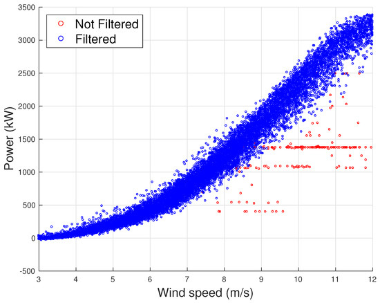 Figure 2. Example of raw and filtered power curve data of T1.
3. Methods
3.1. SCADA Data Analysis
The basis for the SCADA data analysis is constituted by the binning method. The rationale is that for the purpose of performance analysis, the average behavior of a wind turbine is likely sufficient to highlight an apparent anomaly. The critical point is instead given by the interpretation of the apparent under-performance, and here is where the approach proposed in this study intervenes.
The principles of the binning method can be summarized starting from the power curve analysis. The power curve is the relation between the wind speed v and the power P. The design specifications of a wind turbine indicate that this relation should be a line; however, in a real-world environment, it is instead a cloud of points. Therefore, the simplest method for a space–time comparison is the binning method applied to the power curve, which reduces a cloud of points to an average line. The method simply consists of grouping the measurements in intervals of wind speed, whose amplitude is typically selected based on plausibility arguments as 0.5 or 1 m/s. Therefore, a given data set is divided accordingly into J subsets having a population of , with . For each, the average power is computed as in Equation (2):
where is the i-th power measurement in the j-th wind speed bin. Therefore, the binning method results in a set of points identifying a line in the plane.
Based on Equation (1), it is recommended that the nacelle wind speed v be renormalized by considering the effect of air density, as indicated in Equations (3) and (4):
where is the corrected wind speed, is the air density measured on site, is the air density in standard conditions, is the absolute temperature in standard conditions (288.15 K), and is the absolute ambient temperature measured on site. This procedure is fundamental in order to compare the observed power curve against the design specifications or in order to perform a time comparison by referring the measurements to a common benchmark (standard conditions). The renormalization is less fundamental when performing a space comparison during a given period because it is supposed that nearby wind turbines are subjected to reasonably similar conditions. Regarding this point, the literature also provides more complex renormalization methods [10,24] based on statistical analysis or design specifications in order to compensate for the absence of a ground-truth reference.
In the present study, two generalizations of the application of the binning method are proposed to interpret a more in-depth performance of the wind farm under investigation.
The former generalization is given by the analysis of operation curves that do not involve wind speed. Some of them have been methodologically explored in [16] and applied in [25] to the long-term analysis of wind turbine performance. These are, for example, the rotor speed–power curve, or the gearbox speed–power curve or the blade pitch–power curve. Since a wind turbine is substantially controlled by regulating the blade pitch and, consequently, the rotor speed, an under-performance should, in principle, be individuated as diminished extracted power for a given rotational speed or, in the partial load region, as increased blade pitch for extracting a certain power. Technically, this requires adapting the binning method from the couple to , where and can be an arbitrary couple of quantities that are considered representative of the wind turbine behavior. As a rule of thumb for individuating the bins, the 10% of the range that assumes is a reasonable bin amplitude.
The latter generalization of the binning method proposed in this study is based on the idea that a wind turbine’s under-performance could likely be individuated as a decrease of the relative performance with respect to a reference wind turbine (which can be selected as the nearest one, for example). For this analysis, the binning method can be applied by selecting to be the power of a reference wind turbine and the power of the target wind turbine. For the application to the test case of interest, is selected as the power of the T5 reference wind turbine and as the power of the target T4 wind turbine. The applications of the binning method employed in this study are therefore summarized in Table 1.

Table 1.
Applications of the binning method.
3.2. Numerical Simulations
CFD (Computation Fluid Dynamics) simulations of the wind field on the actual terrain have been performed using the RANS (Reynolds-Average Navier–Stokes) approach with the WindSim software. The selection of the computational method has been based on the fact that the objective is to inquire if there is a systematic error in the wind speed measurements of one or more wind turbines. Therefore, a numerical simulation, which provides an average picture of the flow field, is sufficient for the scope, and there is no need to employ more sophisticated methods like Large-Eddy Simulations [26]. Furthermore, in general, the WindSim software is widely used in the wind energy practitioners community and for research purposes, as well [27,28,29].
The RNG k- turbulence model has been employed. The selection of RNG k- is based on its good capability of capturing terrain effects [30]. Furthermore, it is the most used and validated in RANS simulations for the mean flow in the Atmospheric Boundary Layer, which has been considered adequate for the purposes of this work (characterization of the mean flow). The calculation domain has been initialized using the ASTERDEM terrain digital information and the European Corine Land use map for roughness estimation. The digital terrain model and the calculation grid are represented respectively in Figure 3 and Figure 4, while the details of the grid (for a total number of 3,492,480 cells) are reported in Table 2. The overall domain size is km in the East–West and North–South directions. The boundary profile is logarithmic, which means it assumes an infinite flat terrain upstream from the calculation domain. The standard setting of 500 m for the boundary layer height has been used in the present study. The boundary condition on top of the domain is constant pressure, and the non-equilibrium log-law wall functions are employed near the ground.
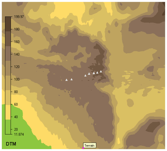
Figure 3.
Digital terrain model.
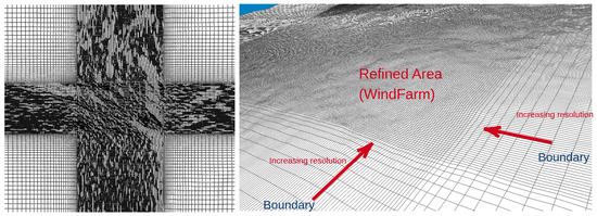
Figure 4.
Grid resolution in the horizontal plane: from the boundary to the investigated area (WindFarm), the spacing is refined from 270 to 17 m.
Table 2.
Grid specifications.
The numerical CFD calculations have been performed blowing the wind on the terrain considering twelve direction sectors and a neutral atmosphere on top of the boundary layer (600 m of height). Two wind regimes have been simulated:
- Low: 10 m/s;
- High: 13 m/s.
Nevertheless, from a practical point of view, it is clear from the wind rose reported in Figure 5 that the most important sectors are 150 and 330 and the results are presented mostly for these two sectors.
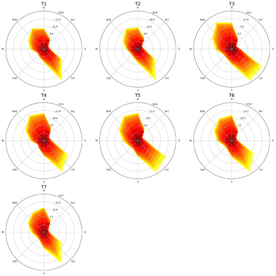
Figure 5.
Wind speed directional distributions on the turbines.
The wind speed and wind shear profiles for the most important wind direction sectors are reported in Figure 6 and Figure 7.
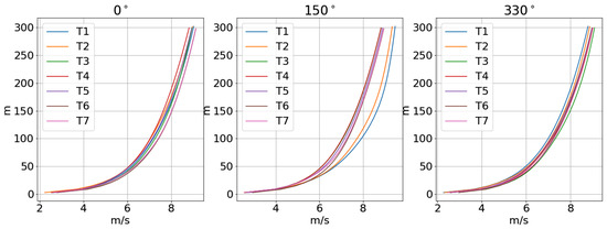
Figure 6.
Wind speed profile for the , , and direction sectors.
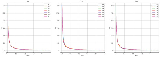
Figure 7.
Wind shear profile for the , , and direction sectors.
The validation of the numerical model is summarized in Table 3 and Table 4, where the average wind speed for the low and high wind speed regimes is compared against SCADA measurements upon averaging on all the wind turbines. The maximum average absolute error is in the order of 1%, which indicates a very good agreement.
Table 3.
Average measured and simulated wind speed: low wind regime.
Table 4.
Average measured and simulated wind speed: high wind regime.
Finally, the adopted procedure goes as follows:
- one turbine is selected as a reference for the wind speed measurement;
- SCADA data are filtered when the wind direction is within the wind sector of interest, and the nacelle wind speed at the reference wind turbine is equal to the one calculated by the CFD model, with a tolerance of 0.2 m/s;
- the difference between the measured and the numerical wind speed are computed (absolute and in percentage) for all the other wind turbines in the farm;
- the above steps are repeated, changing the reference turbine each time: eventually, an error matrix has been obtained.
The rationale for this analysis is that if there is a systematic error affecting one wind turbine anemometer, it can be individuated by the mismatch between measurements and model estimates when the model is set up on the measurements of the other wind turbines in the farm, and vice versa.
4. Results
4.1. SCADA Data Analysis
A preliminary space–time comparison is pursued through the analysis of the power curve, computed using the binning method as indicated in Table 1. Figure 8 reports the power curves of all the wind turbines in the wind farm for 2016 and 2021, respectively. It clearly appears that T4 appears to be underperforming in 2021, while it did not do so in 2016. Therefore, a time comparison of the power curve is performed for T4 (the target wind turbine) and for a reference one (selected to be T5). The results are reported in Figure 9, from which it appears that the power curve of T4 apparently degrades in time, with an abrupt change occurring in 2020, while this does not happen for wind turbine T5.
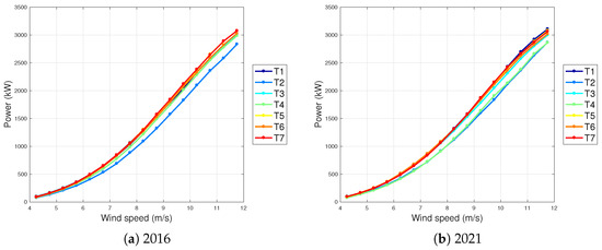
Figure 8.
Power curve for the whole wind farm, computed using the binning method.
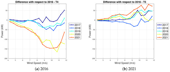
Figure 9.
Difference of the power curve with respect to 2016, for wind turbines T4 and T5.
Given the above results, Figure 10 reports a space–time comparison of the rotor speed–power curves of the wind farm in 2016 and 2021. From this figure, it appears that each wind turbine extracts averagely the same amount of power for a given average rotor speed. The same kind of conclusion about the operational behavior arises from Figure 11 and Figure 12, where the gearbox speed–power curves and the rotor speed–blade pitch curves are reported for the same periods.
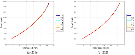
Figure 10.
Rotor speed–power curve for the whole wind farm, computed using the binning method.
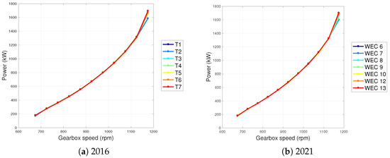
Figure 11.
Gearbox speed–power curve for the whole wind farm, computed using the binning method.
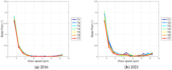
Figure 12.
Rotor speed–blade pitch curve for the whole wind farm, computed using the binning method.
From Figure 10 and Figure 11, it appears that, given a certain rotational speed, wind turbine T4 extracts, on average, the same amount of power as the other wind turbines. At this stage, two hypotheses are conceivable: wind turbine T4 has a lower rotor speed and different blade pitch for a given wind intensity (with respect to the other wind turbines on the farm), which means there is under-performance or an issue with the wind speed measurement. In order to discriminate between these two hypotheses, the binning method is applied to the analysis of the power of the target wind turbine T4 relative to that of reference wind turbine T5. The results are reported in Figure 13 and indicate that the difference in the relative behavior of T4 with respect to T5 is practically negligible (few kW) from 2016 to 2021, while Figure 8 indicates that over those five years, T4 has worsened with respect to T5 up to more or less 10%. This contradiction suggests that the most plausible hypothesis is that wind turbine T4 is affected by anemometer bias. Finally, in Figure 14, the average power curve of the wind farm for 2022 is reported. It appears that, upon replacement of the nacelle anemometer at wind turbine T4, the apparent anomaly has largely been reduced.
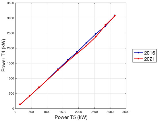
Figure 13.
Power of T4 as a function of the power of T5, computed using the binning method: 2016 and 2021.
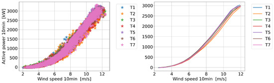
Figure 14.
Power curve for the whole wind farm, computed using the binning method: 2022, upon nacelle anemometer replacement at wind turbine T4.
A deeper insight into the diagnosis of the problem at T4 is provided by the results of the numerical simulations, reported in Section 4.2.
4.2. Numerical Simulations
The results of the comparison between numerical simulations and measurements for 2021 are summarized in Figure 15. The matrix is meaningful because it indicates straightforwardly that wind turbines T2 and T4 are anomalous. The sign of the anomaly is fundamental in order to interpret the results. If the model is tuned to the nacelle anemometer of T2 or T4, the average wind speed estimated at the nacelle of the other wind turbines is higher than the real one for all the wind turbines on the farm. This means that there is a bias at the nacelle anemometers of T2 and T4, which measure a wind speed higher than the actual. From Figure 16, it appears that the error in the wind speed estimation with respect to T4 diminishes considerably upon the replacement of the nacelle anemometer. This is corroborated as well by Figure 17 and Figure 18, where the average absolute errors between the model and measurements are reported for the low and high wind speed regimes. The change in the behavior of T4 upon nacelle anemometer replacement is evident.
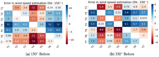
Figure 15.
Percentage error in the wind speed estimation before the replacement of the T4 nacelle anemometer: low wind regime. In the i-th row, the results are obtained by calibrating the model on the nacelle wind speed of the i-th wind turbine.
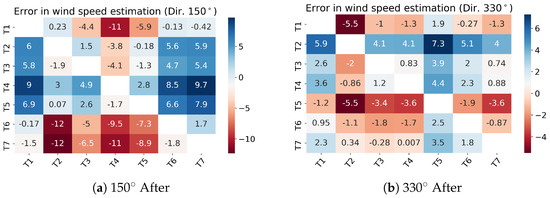
Figure 16.
Percentage error in the wind speed estimation upon the replacement of the T4 nacelle anemometer: low wind regime. In the i-th row, the results are obtained by calibrating the model on the nacelle wind speed of the i-th wind turbine.
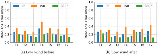
Figure 17.
The mean absolute error between simulation and measurements for the sectors , and , before and after the replacement of the T4 nacelle anemometer: low wind regime.
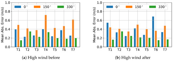
Figure 18.
The mean absolute error between simulation and measurements for the sectors , and , before and after the replacement of the T4 nacelle anemometer: high wind regime.
A careful analysis of Figure 15 and Figure 16 indicates that there are strong directional behaviors, and in particular, the sector is quite peculiar because there are differences between two sub-clusters, which are T1-T6-T7 and T2-T3-T4-T5. This interpretation is corroborated by Figure 19, where the average wind direction (as simulated by tuning the model iteratively on each wind turbine) is compared against SCADA measurements. While the model predicts minimal deviations from one turbine site to the other, the measured wind turbine nacelle direction changes up to from one turbine site to the other.
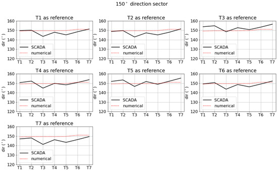
Figure 19.
Comparison between simulation and measurements regarding the average wind direction, where each wind turbine is selected iteratively for tuning the model.
5. Conclusions
The objective of the present study has been to formulate an innovative approach for wind turbine performance analysis and interpretation. As discussed in Section 1, the comprehension of wind turbine performance is characterized by several critical points that deal with data analysis and with measurements. In a nutshell, the power curve of a wind turbine is site dependent and affected by the operation status of the machine. There is no precise ground truth, and the power curve provided by design specifications is useful only to a certain extent. Furthermore, the power of a wind turbine has a multivariate dependence on ambient conditions and working parameters.
Given these considerations, the most innovative approaches in the literature treat the real-world comprehension of wind turbine performance as an issue of space–time comparison [14], to which the present study has contributed through the combined use of SCADA data analysis and CFD simulations. The rationale for this approach is to separate the analysis of the wind field and of the working behavior of the wind turbine and to interpret the results holistically. Based on this, the present study has been organized as a real-world test case discussion regarding a situated wind farm owned by the Fera company.
An important conclusion of the present study is that a robust comprehension of wind turbine performance also requires analysis methods that do not employ wind speed measurements. Two types have been employed in this test case study and are recommended in general. These are the analysis of operation curves (as rotor speed–power or blade pitch–power) and of the relative performance between nearby wind turbines. A general recommendation arising from this work is that the use of CFD simulations for performance analysis is overlooked in the wind energy industry. The test case considered in this work indicates that a RANS free flow model on the actual terrain provides information that can be very useful for understanding the operational behavior of a wind farm. The practical conclusion has been that, based on the analyses of the present work, a nacelle anemometer bias has been individuated and fixed.
The most straightforward further direction of this work is incorporating the rotor orientation in the comparison between numerical modeling and SCADA-collected measurements. This could help interpret the static and dynamic wind turbine yaw behavior, which would be a decisive step forward in improving wind farm operation.
Author Contributions
Conceptualization, F.C. and D.A.; Methodology, F.C., F.N. and D.A.; Formal analysis, D.A.; Investigation, F.C. and R.P.; Data curation, F.C., D.A. and F.N.; Writing—original draft, D.A.; Writing—review & editing, F.C., R.P. and F.B.; Supervision, F.B. All authors have read and agreed to the published version of the manuscript.
Funding
This research received no external funding.
Conflicts of Interest
The authors declare no conflict of interest.
References
- Astolfi, D.; Pandit, R.; Terzi, L.; Lombardi, A. Discussion of wind turbine performance based on SCADA data and multiple test case analysis. Energies 2022, 15, 5343. [Google Scholar] [CrossRef]
- Honrubia, A.; Vigueras-Rodríguez, A.; Gómez-Lázaro, E. The influence of turbulence and vertical wind profile in wind turbine power curve. In Progress in Turbulence and Wind Energy IV; Springer: Berlin/Heidelberg, Germany, 2012; pp. 251–254. [Google Scholar]
- Hedevang, E. Wind turbine power curves incorporating turbulence intensity. Wind Energy 2014, 17, 173–195. [Google Scholar] [CrossRef]
- Pandit, R.K.; Infield, D.; Carroll, J. Incorporating air density into a Gaussian process wind turbine power curve model for improving fitting accuracy. Wind Energy 2019, 22, 302–315. [Google Scholar] [CrossRef]
- Troldborg, N.; Andersen, S.J.; Hodgson, E.L.; Meyer Forsting, A. Brief communication: How does complex terrain change the power curve of a wind turbine? Wind Energy Sci. 2022, 7, 1527–1532. [Google Scholar] [CrossRef]
- Astolfi, D.; Pandit, R.; Gao, L.; Hong, J. Individuation of Wind Turbine Systematic Yaw Error through SCADA Data. Energies 2022, 15, 8165. [Google Scholar] [CrossRef]
- Astolfi, D.; Castellani, F.; Becchetti, M.; Lombardi, A.; Terzi, L. Wind Turbine Systematic Yaw Error: Operation Data Analysis Techniques for Detecting It and Assessing Its Performance Impact. Energies 2020, 13, 2351. [Google Scholar] [CrossRef]
- Rabanal, A.; Ulazia, A.; Ibarra-Berastegi, G.; Sáenz, J.; Elosegui, U. MIDAS: A benchmarking multi-criteria method for the identification of defective anemometers in wind farms. Energies 2019, 12, 28. [Google Scholar] [CrossRef]
- Amato, A.; Heiba, B.; Spertino, F.; Malgaroli, G.; Ciocia, A.; Yahya, A.M.; Mahmoud, A.K. An Innovative Method to Evaluate the Real Performance of Wind Turbines with Respect to the Manufacturer Power Curve: Case Study from Mauritania. In Proceedings of the 2021 IEEE International Conference on Environment and Electrical Engineering and 2021 IEEE Industrial and Commercial Power Systems Europe (EEEIC/I&CPS Europe), Bari, Italy, 7–10 September 2021; pp. 1–5. [Google Scholar]
- Carullo, A.; Ciocia, A.; Malgaroli, G.; Spertino, F. An Innovative Correction Method of Wind Speed for Efficiency Evaluation of Wind Turbines. Acta IMEKO 2021, 10, 46–53. [Google Scholar] [CrossRef]
- Lydia, M.; Kumar, S.S.; Selvakumar, A.I.; Kumar, G.E.P. A comprehensive review on wind turbine power curve modeling techniques. Renew. Sustain. Energy Rev. 2014, 30, 452–460. [Google Scholar] [CrossRef]
- Barber, S.; Hammer, F.; Tica, A. Improving Site-Dependent Wind Turbine Performance Prediction Accuracy Using Machine Learning. ASCE-ASME J. Risk Uncertain. Eng. Syst. Part B Mech. Eng. 2022, 8, 021102. [Google Scholar] [CrossRef]
- Ackermann, T. Wind Power in Power Systems; John Wiley & Sons: Hoboken, NJ, USA, 2005. [Google Scholar]
- Ding, Y.; Kumar, N.; Prakash, A.; Kio, A.E.; Liu, X.; Liu, L.; Li, Q. A case study of space–time performance comparison of wind turbines on a wind farm. Renew. Energy 2021, 171, 735–746. [Google Scholar] [CrossRef]
- Astolfi, D.; Castellani, F.; Terzi, L. Mathematical methods for SCADA data mining of onshore wind farms: Performance evaluation and wake analysis. Wind Eng. 2016, 40, 69–85. [Google Scholar] [CrossRef]
- Astolfi, D. Wind Turbine Operation Curves Modelling Techniques. Electronics 2021, 10, 269. [Google Scholar] [CrossRef]
- Lee, G.; Ding, Y.; Xie, L.; Genton, M.G. A kernel plus method for quantifying wind turbine performance upgrades. Wind Energy 2015, 18, 1207–1219. [Google Scholar] [CrossRef]
- Hwangbo, H.; Ding, Y.; Eisele, O.; Weinzierl, G.; Lang, U.; Pechlivanoglou, G. Quantifying the effect of vortex generator installation on wind power production: An academia-industry case study. Renew. Energy 2017, 113, 1589–1597. [Google Scholar] [CrossRef]
- Morrison, R.; Liu, X.; Lin, Z. Anomaly detection in wind turbine SCADA data for power curve cleaning. Renew. Energy 2021. [Google Scholar] [CrossRef]
- De Caro, F.; Vaccaro, A.; Villacci, D. Adaptive wind generation modeling by fuzzy clustering of experimental data. Electronics 2018, 7, 47. [Google Scholar] [CrossRef]
- Pandit, R.K.; Infield, D. Comparative assessments of binned and support vector regression-based blade pitch curve of a wind turbine for the purpose of condition monitoring. Int. J. Energy Environ. Eng. 2019, 10, 181–188. [Google Scholar] [CrossRef]
- Qu, F.; Liu, J.; Ma, Y.; Zang, D.; Fu, M. A novel wind turbine data imputation method with multiple optimizations based on GANs. Mech. Syst. Signal Process. 2020, 139, 106610. [Google Scholar] [CrossRef]
- Martinez-Luengo, M.; Shafiee, M.; Kolios, A. Data management for structural integrity assessment of offshore wind turbine support structures: Data cleansing and missing data imputation. Ocean Eng. 2019, 173, 867–883. [Google Scholar] [CrossRef]
- Carullo, A.; Castellana, A.; Vallan, A.; Ciocia, A.; Spertino, F. In-field monitoring of eight photovoltaic plants: Degradation rate over seven years of continuous operation. Acta IMEKO 2018, 7. [Google Scholar] [CrossRef]
- Astolfi, D.; Byrne, R.; Castellani, F. Analysis of Wind Turbine Aging through Operation Curves. Energies 2020, 13, 5623. [Google Scholar] [CrossRef]
- Porté-Agel, F.; Wu, Y.T.; Lu, H.; Conzemius, R.J. Large-eddy simulation of atmospheric boundary layer flow through wind turbines and wind farms. J. Wind Eng. Ind. Aerodyn. 2011, 99, 154–168. [Google Scholar] [CrossRef]
- Sebastiani, A.; Castellani, F.; Crasto, G.; Segalini, A. Data analysis and simulation of the Lillgrund wind farm. Wind Energy 2021, 24, 634–648. [Google Scholar] [CrossRef]
- Tabas, D.; Fang, J.; Porté-Agel, F. Wind energy prediction in highly complex terrain by computational fluid dynamics. Energies 2019, 12, 1311. [Google Scholar] [CrossRef]
- Song, Y.; Paek, I. Prediction and Validation of the Annual Energy Production of a Wind Turbine Using WindSim and a Dynamic Wind Turbine Model. Energies 2020, 13, 6604. [Google Scholar] [CrossRef]
- Peralta, C.; Nugusse, H.; Kokilavani, S.; Schmidt, J.; Stoevesandt, B. Validation of the simplefoam (rans) solver for the atmospheric boundary layer in complex terrain. ITM Web Conf. 2014, 2, 01002. [Google Scholar] [CrossRef]


Disclaimer/Publisher’s Note: The statements, opinions and data contained in all publications are solely those of the individual author(s) and contributor(s) and not of MDPI and/or the editor(s). MDPI and/or the editor(s) disclaim responsibility for any injury to people or property resulting from any ideas, methods, instructions or products referred to in the content. |
© 2023 by the authors. Licensee MDPI, Basel, Switzerland. This article is an open access article distributed under the terms and conditions of the Creative Commons Attribution (CC BY) license (https://creativecommons.org/licenses/by/4.0/).