Abstract
The rapid development of natural gas pipelines has highlighted the need to utilize SCADA (supervisory control and data acquisition) system data. In this paper, a heat transfer model of a natural gas pipeline based on data feature extraction and first principle models, which makes full use of the measured temperatures at each end of the pipeline, is proposed. Three methods, the NARX neural network (nonlinear autoregressive neural network with exogenous inputs), time series decomposition, and system identification, were used to model the changes of gas temperatures of the pipeline. The NARX neural network method uses a cyclic neural network to directly model the relationship of temperature between the start and the end of the pipeline. The measured temperature series at the pipeline inlet and outlet were decomposed into trend items, fluctuation items, and noise items based on the time series decomposition method. Then the three items were fitted separately and combined to form a new temperature prediction series. The system identification method constructed the first-order and second-order transfer function to model the temperature. The simulation of the three data-driven models was compared with those of the physics-based simulation models. The results showed that the data-driven model has great advantages over the physics-based simulation models in both accuracy and efficiency. The proposed models are more suitable for applications such as online simulation and state observation of long-distance natural gas pipelines.
1. Introduction
Natural gas, as a stable, low-cost, high-calorific green energy, plays an important role in protecting the ecological environment and transitioning from fossil energy to clean energy. As natural gas is a low-density, compressible fluid, pipeline transportation is the most economical way for long-distance transportation. As the natural gas pipeline network becomes larger, research development on reliability [1], design [2], and operation optimization [3] is necessary, as well as the simulation of natural gas pipeline networks, to accurately reproduce the distribution of gas pressure, temperature, and flow in the pipeline, and carry out pipeline network design planning and operation scheduling based on these parameters. The conventional numerical simulation method of the natural gas pipeline is to establish a mathematical model according to the mass, momentum, and energy conservation equations, and then use a suitable numerical method to solve the equations [4]. The choice of different mathematical models and numerical solutions determines the precision and accuracy of the simulation method [5,6]. For the hydraulic equation centered on the mass equation and the momentum equation, the common simplification method is to ignore the inertial term in the momentum equation. The studies found that the neglect of the inertial term will lead to large errors in the case of fast transients [7]. The thermodynamic equation dominated by the energy equation has often been simplified by isothermal or adiabatic flow process in previous studies. However, the gas state changes with the variation of pressure and temperature, and the assumption of isothermal and adiabatic process is inconsistent with practical engineering, which leads to large errors in the temperature simulation of natural gas pipelines.
With the development of computer technology, the natural gas pipeline simulation, based on the three complete basic equations without simplification, has become mainstream. To solve complex gas pipeline flow equations, there are a variety of numerical methods. The finite difference method is commonly used to discretize the continuous solution domain into a grid of abscissa distance and ordinate time. In the finite volume method [8], the derivative term is integrated into an expression of the state variable of the interface, and the interface value approximated from the local distribution is substituted to obtain a complete discretization equation. The characteristic line method [5] is a method for solving hyperbolic partial differential equations based on characteristic theory, which transforms the partial differential equation into a total differential problem along the characteristic line. The idea of the state space model method [9,10] originates from modern control theory. Based on the Laplace transformation, the time domain functions are converted into frequency domain functions to obtain a set of closed ordinary differential equations. The state space method needs to omit the inertial system of momentum equation and use it under adiabatic or isothermal conditions, with high calculation efficiency and low calculation accuracy.
In recent years, in order to solve the problem that the accuracy and calculation speed of conventional numerical simulation methods cannot be achieved simultaneously, some scholars have begun to use data-driven modeling methods. In 2015, Hadian used neural networks to model the hydraulic steady state of a large natural gas pipeline network, and combined it with a model predictive control algorithm for pressure control [11]. In 2018, based on deep learning algorithms, Su used time windows and autoencoders to predict the operation status of natural gas pipeline networks [12]. In 2020, Cui used the calculation results of neural networks as the initial value in the iterative process of steady-state hydraulic calculation to speed up the calculation [13]. In 2022, Yin adopted the idea of the surrogate model, combined with BP neural networks and genetic algorithms to carry out data-driven modeling and control of natural gas station pipeline networks [14]. At present, the research on data-driven natural gas pipeline simulation technology is still in its infancy. The existing research is mainly based on the steady-state model considering only hydraulics, which are lack of temperature transient models.
In first principle models, the heat exchange between the natural gas in the pipeline and the environment is an important part of the thermal simulation. In some simplified thermal models, it is assumed that the total heat transfer coefficient of the pipeline and the ambient temperature around the pipeline remain unchanged. When Fourier law is used to calculate the heat transfer, the periodic changes of the ambient temperature with time are ignored in this assumption, which makes the description of the temperature field of the pipeline and the surrounding environment deviate, which results in large calculation deviations when it is brought into the thermal equation. Targeting this problem, a transient heat transfer model was developed, which iteratively solves the pipeline problem according to the time and space division, and the calculation results are more accurate than the steady-state model. However, due to the large number of calculations and the inability to obtain the environmental parameters along the line in practical application, it is difficult to apply the algorithm for engineering requirements.
When physics-based simulation models are used to simulate the natural gas temperature, steady-state thermodynamics are used to speed up the calculation, or transient thermodynamics are used to improve the simulation accuracy. Therefore, a data-driven thermal model for long distance natural gas pipelines is proposed in this paper. Using the measured temperature at both ends of the pipeline, three methods, the NARX neural network [15], time series decomposition, and system identification [16,17], are used to model the temperature of the natural gas pipeline. To verify the advantages of different approaches in different aspects, three data-driven models are compared with first principle models in simulation. Finally, the calculation accuracy and applicability of different methods are judged from calculation times and errors.
This paper contributes the following:
To improve the simulation efficiency, this paper proposes an agent simulation method using data-driven methods to simulate the natural gas pipeline outlet temperature, which includes the NARX neural network, time series decomposition, and system identification.
The input parameters of the data-driven model are determined based on the mechanism analysis, which avoids the problem of blind parameter adjustments of the data-driven model and ensures the rationality of the operation and the reliability of the results.
The data-driven methods are verified by a section of the actual operating pipeline, and their simulation error influencing factors are analyzed.
2. First Principle Model
2.1. Gas Flow Model in Pipe
The mathematical description of the flow of natural gas in the pipeline included the continuity equation, Equation (1); the momentum equation, Equation (2); the energy equation, Equation (3); and the gas state equation, Equation (4). The continuity equation and momentum equation primarily solved the hydraulic parameters of natural gas, while the energy equation primarily solved the thermodynamic parameters. The gas state equation was used to describe the relationship between the state of natural gas and the pressure and temperature [18].
where A, x, d, and θ are the cross-sectional area (m2), the axial length of pipeline (m), the inner diameter (m) and the inclination of pipelines, respectively. T is time(s). T, p, v, and ρ are the temperature (K), pressure (Pa), velocity (m/s), and density (kg/m3) of natural gas, respectively. λ is the friction factor. g is gravitational acceleration. e is the specific internal energy (J/kg). h is the specific enthalpy (J/kg). Qq is the heat transfer between the natural gas and the ambient environment (J/kg). Z is the compressibility factor.
2.2. Thermal Model
Early gas pipeline flow simulations were carried out under isothermal or adiabatic assumptions. Increasing research has led to the development of various temperature models based on energy equations. There are three types of commonly used models: the steady flow model based on the Sukhov formula, the heat transfer model based on steady heat transfer, and the heat transfer model based on transient heat transfer.
2.2.1. Sukhov Formula
The Sukhov formula is recognized as the temperature equation in the pipeline design in the field of oil and gas storage and transportation engineering. It can be deduced directly from Equation (3) under stable flow conditions.
For steady flow, the temperature drop equation along the natural gas pipeline is as follows:
where T0 is the ambient temperature (K). Tq is the pipe inlet temperature (K). a is , while M is the mass flow (kg/s), cp is the specific capacity heat in constant pressure (J·kg−1K−1). Di is the throttling effect coefficient (K/Pa).
The last item of Equation (5) considers the temperature drop caused by the Joule–Thomson effect. If the influence of this item is ignored, the Sukhov formula is obtained:
Since this formula only considers the stable flow of natural gas, it simplifies the actual gas flow process in the pipe. Although it is still used in engineering, the calculation results of high pressure and unstable flow conditions have large errors.
2.2.2. Steady-State Heat Transfer Model
The heat transfer between the gas in the tube and the surrounding environment is an important part of the thermal simulation. In the energy equation, the heat transfer term Q represents the heat transfer between the unit mass of natural gas and the surrounding environment. In most thermal models, it is considered that the pipeline and the surrounding environment are in a steady state, which means that the surrounding environment temperature is constant, and the thermal conductivity of the pipe material and the surrounding environment are unchanged.
Fourier’s law Equation (7) is applied to calculate the total heat transfer between a certain section of natural gas and the environment:
where Kall is the heat transfer coefficient (W/(m2·K)).
This formula can be further rewritten as:
The expression Kall/πD of K(W/m2·K) represents the total heat transfer coefficient between the pipe with diameter D and the environment, which is also the total heat transfer coefficient between the gas and the surrounding ground [19].
2.2.3. Transient State Heat Transfer Model
The accurate description of the heat transfer phenomenon of natural gas pipelines requires analysis of multiple factors. The heat transfer of natural gas pipelines in the above steady-state model description is one-dimensional heat transfer, and there is no description of the ground characteristics and ambient temperature changes near the pipelines. In fact, due to the heat storage effect of the environmental medium, the temperature of the surrounding environment and the pipe wall after heat exchange is not a constant value, but a radial temperature field with the pipe as the axis. Moreover, the pipe wall of a natural gas pipeline is composed of a steel layer, a thermal insulation layer, and an anticorrosion layer. The transient heat exchange model considering the heat storage capacity of multilayer structure is shown as Equation (9) [20].
In the calculation of the model, not only the change of temperature with the radial temperature of the pipe, but also the change of temperature of each layer with time and the heat exchange process between gas and the inner wall of the pipe, were considered. Previous studies [20,21,22] show that the calculation accuracy of the transient heat transfer model is higher than that of the steady-state heat transfer model. However, the calculation of the transient heat transfer model greatly increases the calculation amount of thermal simulation, and it is difficult to determine the temperature and heat transfer characteristics of different formations, so the transient heat transfer model is rarely used in the simulation of gas temperature change.
2.2.4. Thermohydraulic Simulation of a Natural Gas Pipeline Based on the FVM
There are three common methods used in gas pipeline simulations: the method of characteristics (MOC), the finite difference method (FDM), and the finite volume method (FVM). When comparing the results of the MOC and the FVM under fast and slow transients in a single natural gas pipeline, the FVM outperforms the MOC in both aspects. Therefore, the FVM with staggered grids is used for natural gas thermohydraulic simulation. According to thermodynamic law, the energy equation Equation (4) is converted as follows:
Equations (1), (2) and (10) constitute the control equations for the natural gas pipeline simulation.
The control equations are discretized using FVM on staggered grids (Figure 1) [8]. Among the main variables, the velocity variable is located at the edge of the grid and is marked with a virtual line. The pressure and temperature variables are located in the center of the grid and are marked with black dots. Density, heat capacity, and other physical parameters are also located in the center of the grid.
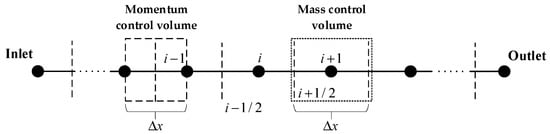
Figure 1.
Schematic diagram of pipe grid division.
The momentum equation Equation (2) is discretized in the momentum control volume, and the continuity equation Equation (1) and energy equation Equation (10) are discretized into the following equations, respectively, in the mass control volume:
where superscript # represents the current value of the variable, and * represents the value to be solved in the next iteration of the variable.
Using to the discrete equation of FVM, the overall pipeline simulation process, which solves the transient hydrothermal state of natural gas pipeline by a numerical method, is shown in Figure 2 [8].
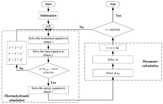
Figure 2.
The FVM numerical solution process.
2.3. Model Comparison
2.3.1. Basic Data
In order to systematically compare the differences in numerical accuracy and calculation speed of the three thermal models based on first principle models, a section of an actual natural gas pipeline was used in this paper. The differences in numerical accuracy and calculation speed of different methods were analyzed by comparing the numerical results and CPU time under the same calculation conditions. The pipeline parameters, pipe wall properties, and gas composition are shown in Table 1, Table 2 and Table 3.

Table 1.
Pipeline parameters.
Table 2.
Properties of pipe wall.
Table 3.
Gas composition.
The 12-hour operation data of the pipeline were obtained through the supervisory control and data acquisition (SCADA) system, and the boundary data of simulation calculations were determined, including the exit pressure, flow rate, the temperature of the first station, and the entry pressure of the last station. The conditions of inlet and outlet pressure (Figure 3) and inlet temperature (Figure 4) are as follows:
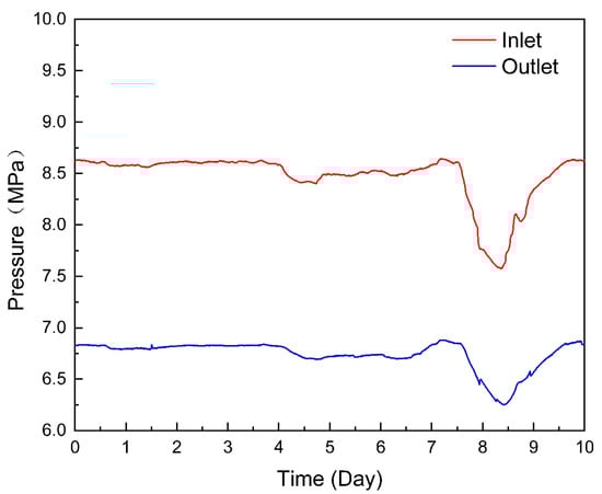
Figure 3.
Inlet and outlet pressure.
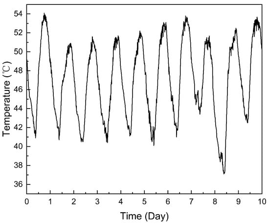
Figure 4.
Inlet Temperature.
The selected pipeline was in stable operation from one to seven days, with a steady inlet and outlet pressure, temperature affected by day and night temperature differences, and an air cooler cooling efficiency showing periodic regular fluctuations. After the eighth day, due to the increase of gas consumption of downstream users, the reduction of gas storage in the pipe led to an abnormal pressure drop in the whole line.
2.3.2. Comparison of First Principle Models
In this paper, the hydrothermal simulation of steady-state heat transfer model and transient heat transfer model was realized based on the finite volume method under a staggered grid. The calculation parameter settings and calculation time of this example are shown in Table 4.
Table 4.
Grid calculation parameters.
The grid spacing was 1 km, the time step was 10 s, and the simulation was performed for 10 days. By solving the two types of first principle models, the results of the hydraulic simulation and thermal simulation of the natural gas pipeline could be obtained. The comparison between the calculated outlet flow rate and temperature is shown in the Figure 5 and Figure 6:
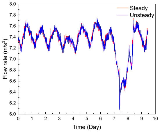
Figure 5.
Flow rate comparison.
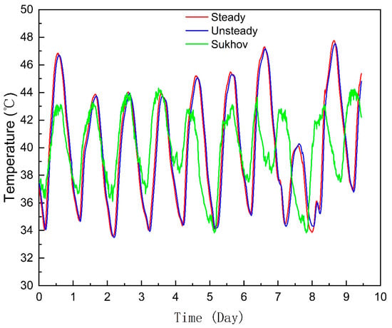
Figure 6.
Temperature comparison.
Figure 5 and Figure 6 demonstrate that under the same boundary conditions, whether through hydraulic simulation or thermal simulation, the calculation results of the steady-state model and the transient model are basically consistent, while the temperature results calculated by the Sukhov formula have large errors. The reason is that the transient model considers the relationship between the radial temperature field with the axis of the pipe and time and space, while the steady model converts the heat transfer of the pipe into a one-dimensional heat transfer problem, making its errors relatively large. The Sukhov formula considers that the temperature distribution along the natural gas pipeline is constant during operation. The steady model converts the heat transfer of the pipeline into a one-dimensional heat transfer problem to be solved. The total heat transfer coefficient takes the total heat transfer coefficient as a constant to solve, which has less parameters and a faster calculation speed. The transient model considers the heat capacity and temperature change of each layer of the pipeline. Therefore, in the process of solving the heat transfer coefficient, multiple differential equations, which are based on the known heat transfer parameters, such as soil type, geographical location, etc., needed to be solved.
The error vector can be calculated from the data in Figure 6 and the formula for calculating the absolute value of the relative error, and the error comparison between the steady-state model and the transient model can be obtained, as shown in Table 5:
Table 5.
Comparison of physical model.
The results show that the simulation result of the transient model was better than the steady model. Therefore, this paper uses the simulation results of transient state heat transfer model as a reference for comparison of various methods for the following two reasons: (1) For the unsteady-state heat transfer model, it is necessary to determine the parameters such as soil type, fuel depth, and geographic location. It is difficult to identify these unsteady-state heat transfer model parameters simultaneously. (2) The amount of heat transferred to the ground in the steady model can be close to the calculated value of the unsteady model by modifying the total heat transfer coefficient [23]. The steady-state model is often used for thermohydraulic simulation when gas temperatures need to be calculated quickly. In addition, the steady and transient models rely on hydraulic calculation to solve the temperature, which is the fundamental reason for the calculation time.
3. Data-Driven Model Construction
For the simulation of gas temperature change, it is difficult to determine the environmental parameters of the buried depth of the pipeline and pipeline parameters required in the simulation of the first principle model, which creates extensive difficulties in the calculation of the first principle model. For thermal simulation, the temperature change at the outlet point of natural gas is affected by many factors such as the temperature change at the upstream point and the ambient temperature change. Therefore, this paper adopts a data-driven method to explore mapping the relationship between the upstream and outlet temperatures of the pipeline. Common data-driven modeling methods include neural networks, time series analyses, and system identification.
3.1. NARX Neural Network
3.1.1. NARX Neural Network Introduction
As a dynamic neural network, NARX has a memory function [24]. It retains the information of the last moment, which not only makes full use of data information but also improves its ability to solve complex problems. For the complex factors affecting the gas temperature change in the natural gas pipeline, the mathematical model parameters are numerous and difficult to determine, so a nonlinear autoregressive model with time series was established.
The NARX network is an external input nonlinear autoregressive neural network, which can fit the nonlinear system approximation function well. Its mathematical description is:
where ŷ is the predicted output of NARX, which can be represented as a function of exogenous inputs (x(t − 1), …, x(t − d1)) and endogenous inputs (ŷ(t − 1), …, ŷ(t − d2)) of the neural network. d1 and d2 are input delay and feedback delay, respectively. The structure of NARX ensures that it includes a time delay in the input to maintain a continuous record of the input data history. The output of hidden layers and output layers of the NARX network are computed by:
where w is the weight of the neural network. b is the bias of the neural network, which include all parameters of NARX during the training procedure. u(t) is output of hidden layers and input of output layers. Subscripts 1 and 2 denote hidden layers and output layers, respectively. Subscript h denotes the history data. xh and ŷh are defined by Equation (17):
Figure 7 shows the structure of the established NARX neural network, where + represents the weighting, and the arrow represents the data flow direction. The outlet temperature of the natural gas pipeline can be determined by the inlet temperature and the inlet and outlet pressure, which was used as the input variable of the NARX neural network. In addition, the outlet temperature at the previous moment was also brought into the calculation as an input variable.
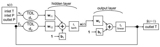
Figure 7.
The NARX neural network structure.
3.1.2. NARX Neural Network Construction
The training methods of the NARX neural network included open-loop and closed-loop. The output of the NARX neural network model trained by open-loop was not fed back to the model for correction, so the fitting results of the model met the law of the training sample set. The NARX neural network trained by closed-loop could feed back the predicted temperature at time t − 1 to the input sample, and combined the input variables (inlet temperature and inlet and outlet pressure) at time t to predict the temperature of natural gas at time t. The specific training methods are as follows:
- The measured pipeline data were divided into a training dataset and a dataset used in the case study, and the dataset used in the case study was a comparison of each method in the article.
- The training data set was normalized, which eliminated the impact of dimensions on model training. Batch normalization was used as the normalization method.
- The training data set was randomly divided into three types of training, verification, and test data, including 70%, 15%, and 15% data, respectively.
- The neural network model was trained. During training, the NARX model used the open structure for training, which means that the measured data were selected for input by the endogenous inputs of NARX.
- After the model training, the endogenous inputs of NARX were adjusted to the output value of NARX at the previous time to complete the closed-loop prediction of the model.
The NARX neural network had three main parameters: input delay, feedback delay, and a number of hidden layers. The input delay and feedback delay determined the different delay steps of the output variable and the input variable to control the time step of continuous prediction; the number of hidden layers determined the training effect of the neural network.
For the settings of the NARX parameters, the input delay was designed by calculating the time required for the pressure wave at the inlet of the pipeline to the outlet. For the feedback delay, the prediction accuracy of the model should first rise and then decline with the increase of output delay. The selected parameters were as follows: input delay (1:80) and feedback delay (1:5). The training datasets were divided into three categories of training, validation, and test data containing 70%, 15%, and 15% of the data, respectively.
Additionally, this paper used the example data of Section 2.3 to test 100 parameter settings and select the delay setting with the best prediction result. The comparison of prediction results was obtained by comparing the average value of the absolute value of the difference between the neural network output and the original data. The average error results of 100 groups of results are shown in Figure 8:
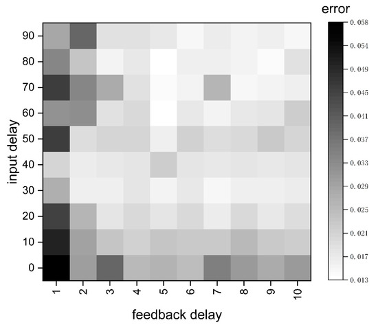
Figure 8.
Average error result.
The comparison results showed that the setting of input delay (1:80) and feedback delay (1:5) had the best simulation effect on temperature. This was approximately the same as the results of parameter settings derived from the mechanistic analysis. In order to ensure that there was no over fitting, the number of hidden layers cannot be too large. In this paper, 10 hidden layers were selected.
Taking the calculation in Section 2.3 as an example, the inlet temperature sequence was used as the input and the outlet temperature sequence was used as the output to train the neural network. The results of the outlet temperatures are shown in Figure 9. The mean absolute error was 0.833 °C, the maximum absolute error was 5.253 °C, and the mean relative error was 1.982%.
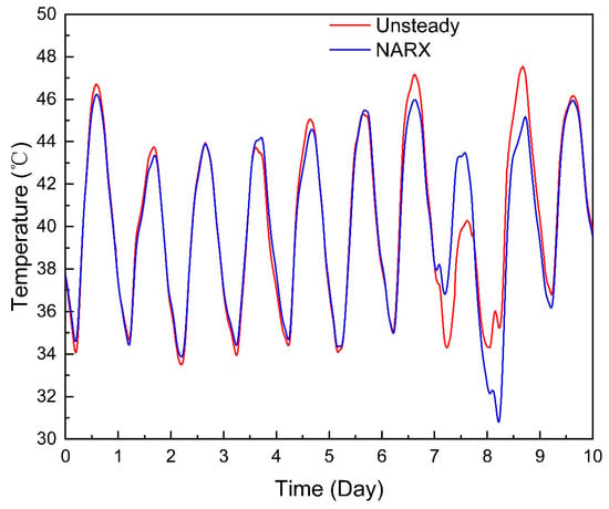
Figure 9.
NARX neural network result.
3.2. Time Series Decomposition
3.2.1. Time Series Decomposition
Because the ambient temperature changes periodically with the season, day and night, and the outlet temperature of natural gas is affected by the upstream temperature changes and the accumulation of upstream temperature changes, the time series of natural gas temperature has many variation characteristics, such as trend, periodicity, and mutagenicity.
In this paper, the temperature time series were decomposed into three parts: the trend item, the fluctuation item, and the noise item. The trend item represents the influence of the environmental temperature cycle change and the temperature cumulative change on the temperature time series, the fluctuation item represents the influence of the upstream temperature fluctuation on the outlet temperature, and the noise item represents the measurement noise of the thermometer. By decomposing the time series and analyzing and studying the variation laws of each item, the variation laws of natural gas temperatures can be better explained.
Let X be the time series, T is the trend item, P is the fluctuation item, and R is the noise item, then X can be expressed as:
- Smooth the temperature time series X through the Savitzky–Golay filter Equation (19), and the difference between the results obtained and the temperature time series is the noise item R, which does not influence the trend item and the fluctuation item.
- The trend item represents the overall trend of the temperature changes in a period of time. Therefore, the trend item represents the overall change of natural gas temperatures over a long period of time. The trend item is obtained by filtering the time series with the mean value of 1000 points, which is the average value of the time required for the inlet temperature changes to transfer to the outlet temperature.
- The temperature time series minus the noise item and the trend item is the fluctuation item.
In the calculation example of Section 2.3, after adding random noise (white noise) to the time series of inlet and outlet temperatures, after performing the above decomposition steps, each subitem can be obtained as shown in Figure 10.
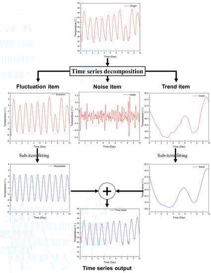
Figure 10.
Time series decomposition results.
3.2.2. Subitem Fitting
In the three decomposition items of the temperature time series, the noise item could be ignored due to the normal distribution with a mean value of approximately zero. The mapping relationship between the trend item and the fluctuation item was carried out by using the least squares method. First, the input and output delays of each subitem were determined, and then the linear mapping was performed, as shown in Equation (20):
Taking the calculation in Section 2.3 as an example, the fitting effect of each subitem is shown in Figure 11, and the total fitting effect of the outlet temperature is shown in Figure 12. The mean absolute error was 0.978 °C, the maximum absolute error was 4.564 °C, and the mean relative error was 2.348%.
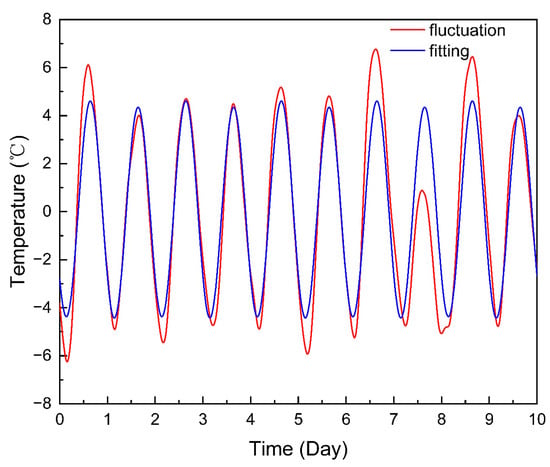
Figure 11.
Subitem fitting.
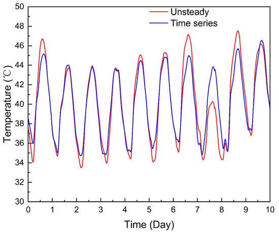
Figure 12.
Total fitting.
3.3. System Identification
System identification is to determine a model equivalent to the measured system from a set of given model classes on the basis of input and output data for a system [25]. The three major elements of system identification are: system input and output data (dataset), model class, and equivalence criterion (criteria function). The relationship is shown in Figure 13.
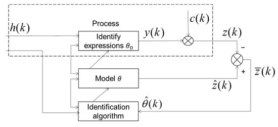
Figure 13.
System identification structure.
In order to obtain the estimated value of the model parameter θ, the step-by-step method is generally used. At time k, the output of the model was calculated according to the estimated parameters of the previous time, and the predicted output value was obtained:
Then the prediction error of the output at time k is:
where the process output
Then, the input h(k) of the identification expression can be calculated. The should be fed back to the identification algorithm, the current model parameter estimation θ(k) under a certain criterion function should be calculated, the model parameters updated, the corresponding criterion function iterated to obtain the minimum value, and then the required model obtained.
The mathematical model obtained by the system identification method was only an equivalent model of the actual pipeline, and could not be completely equivalent to the pipeline object. The model finally obtained was used to represent the data characteristics of the pipeline system and express it in an appropriate form, which could fit the dynamic characteristics of the actual change of natural gas temperature well.
In this paper, the state space model Equation (24) is selected as the input model to describe the gas thermodynamic process system identification. The characteristic of this model is that it cannot only reflect the internal state of the system, but also reflect the relationship between the internal state of the system and the external input and output variables.
Taking the calculation in Section 2.3 as an example, the inlet temperature sequence was used as the input and the outlet temperature sequence was used as the output, and the model was identified. The results of the outlet temperature are shown in Figure 14. The mean absolute error was 1.206 °C, the maximum absolute error was 6.057 °C, and the mean relative error was 3.008%.
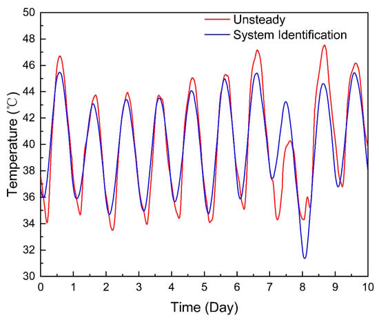
Figure 14.
State space identification result.
4. Data-Driven Model Comparison
4.1. Numerical Accuracy Comparison Method
To quantify the numerical accuracy of the five different forms of thermal simulation, the mean relative error was defined as follows:
where subscript u represents the calculation result of the transient model.
In order to facilitate the comparison of deviations between different methods, the following two forms were used:
The overall deviation of different methods was expressed by the average of the deviation, that is:
The comparison of the calculation accuracy of different methods was carried out using the cumulative error, that is, the cumulative error at the point t = n was the sum of the error at t = 0 to the error at t = n. The purpose of this was to clarify the law of error distribution between different algorithms, and to facilitate the comparison of the size of errors between different algorithms.
4.2. Comparison of Simulation Results of Various Methods
In this paper, the numerical results of the three data-driven models were obtained in Section 3, and the two first principle models were solved in Section 2. The calculation results of the four methods can be compared with the result of the transient state heat transfer model as shown in Figure 15:
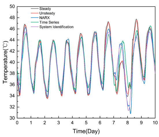
Figure 15.
Comparison of thermal simulation results.
As shown as Figure 15, the calculation results of the two first principle models were consistent with the actual data, and the calculation results of the three data-driven models were very similar to the actual data, but the calculation error was large under some transient working conditions. The reason for this was that the three data-driven models were simulated based on mapping law between the data. The conventional working conditions account for a large proportion in the data, resulting in a large weight of the conventional working conditions when training the model. The data results during the simulation were biased towards the conventional working conditions, resulting in a large error under some working conditions.
Figure 16 and Figure 17 show the overall deviation and cumulative deviation of the five methods used to predict the outlet temperature using the error calculation method given in Section 4.1:
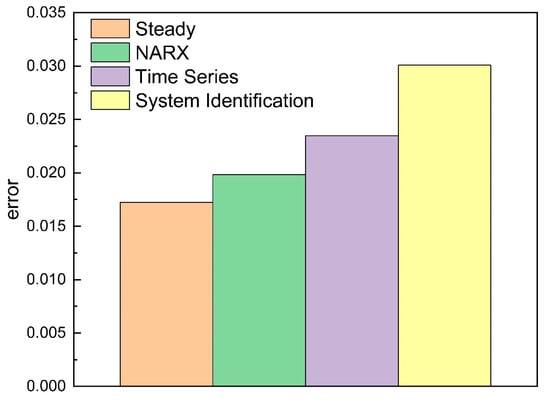
Figure 16.
Overall deviation.
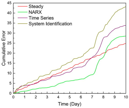
Figure 17.
Cumulative error.
Figure 16 demonstrates that the overall error of the transient simulation results was less than 1%, which was almost consistent with the actual data, while the overall error of the steady-state simulation results and the NARX neural network results was about 2%, and the overall errors of the time series decomposition and the system identification were about 2.5% and 3%, respectively, which is larger than the NARX neural network. Compared with the other two data-driven models, the calculation error of the NARX neural network was small because the output value of the last time was input during training, so it could correct the change of the natural gas outlet temperature caused by external interference, making its error smaller. The results show that when the accuracy requirements of the calculation were not high (<3%), the calculation results of the five methods satisfied the accuracy requirements, and any method could be applied in the operation of a pipeline.
Figure 17 demonstrates that the cumulative errors of the simulation results of the first principle models showed a trend of uniform growth, which was expounded in Section 2.3.2. The errors of the three data-driven models also increased uniformly under normal working conditions, while the cumulative error curves under abnormal working conditions had a clear increasing trend. The cumulative errors of the three data-driven models’ simulation results of 1–7 days all increased evenly. When the abnormal conditions occurred on the eighth day, the cumulative error curve had an obvious sloping increasing trend. The above results showed that data-driven models are highly sensitive to the occurrence of abnormal conditions, but the results still met the requirements for simulation accuracy in the actual operation of a pipeline.
In terms of calculation speed, the same computing equipment was used to calculate the five simulation models, and the simulation times are shown in Table 6. There were two iterative processes in the calculation process of the transient simulation, so in this case (grid spacing 1 km, time step 10 s), the calculation time was 951 s; there was an iterative process in the steady-state simulation calculation process. In this case, the calculation time was 209 s; the calculation time of the three data-driven models was very short, the calculation time of the NARX neural network was 0.0382 s, the calculation time of the time series decomposition was 1.67 s, and the calculation time of the system identification was 0.163 s. The model used for the NARX neural network and system identification has been trained, and the model training still needs some time (NARX 4.00 s, system identification 1.52 s). As the NARX neural network simulation speed was the fastest, it is better to select NARX models for long-term simulation. The calculation speed of the data-driven models was faster than that of the first principle model by comparison.
Table 6.
Comparison of simulation time.
5. Conclusions
Six methods in the thermal simulation of natural gas pipelines were studied in this paper: the Sukhov model, the steady-state heat transfer model, the transient heat transfer model, the NARX neural network method, the time series decomposition method, and the system identification method. The actual cases were designed to compare the simulation accuracy between the physics-based simulation models and the data-driven models. From the numerical results, the following conclusions can be made:
- (1)
- The average simulation errors of the three data-driven models were 1.98%, 2.35%, and 3.01%, which satisfy the requirements for simulation accuracy in pipeline operations. The main accuracy loss of data-driven models occurred under abnormal working conditions, such as a sudden change of ambient temperature and natural gas cooling and transportation, while the calculation accuracy was very high under normal working conditions. Therefore, when the requirements for simulation accuracy are high, the data-driven model can be used for simulation under stable working conditions.
- (2)
- The time calculations of the data-driven models were 4.0382 s, 1.67 s, and 1.683 s, which were faster than that of the first principle model. Among them, the total time of time series decomposition and system identification were almost consistent. The NARX neural network and system identification models need to obtain the applicable model through the analysis of historical data. The time to establish the model was relatively long, while the time series decomposition model was calculated directly, which was shorter than the NARX neural network.
- (3)
- In terms of applicability, the three first principle models did not need to be calculated with actual known data, and have strong applicability to different pipelines, but the physical parameters, such as ambient temperature, thermal conductivity between the pipe and the surrounding environment should be known; the solutions of the three data-driven models were obtained by analyzing the known data. Therefore, the models obtained for different pipelines and even different working conditions were different, and there are requirements for the acquisition of actual data. Too little data will lead to the model output not being in line with the reality, and a large difference in data under different working conditions will also lead to a deviation of calculation capacity under different working conditions.
The numerical results show that data-driven models have high calculation accuracy, high simulation efficiency, and have good applicability to the direction of rapid calculation demand, such as pipeline control engineering and parallel simulation of pipe networks. Moreover, simulation results could replace part of the calculation results of the mechanism model to simplify the complex hydrothermal coupling solution method. The input parameters of the data-driven model were determined based on the physics analysis, which avoided the problem of the blind parameter adjustment of the data-driven model and ensured the rationality of the operation and the reliability of the results.
In future research, sensitivity analysis of input parameters of the data-driven model can identify pipeline parameters. In addition, it is necessary to use the data-driven model as a proxy model to speed up solving the process of thermohydraulic simulation.
Author Contributions
Conceptualization, K.W.; methodology, H.X.; validation, H.X. and W.Q.; investigation, H.L.; supervision, Y.L.; project administration, B.H. All authors have read and agreed to the published version of the manuscript.
Funding
This work was supported by the Science Foundation of the China University of Petroleum, Beijing (No. 2462020YXZZ045) and the research and development of multitime scale flow digitalization system (No. HX20210115).
Informed Consent Statement
Not applicable.
Data Availability Statement
Not applicable.
Acknowledgments
This work is supported by the National Engineering Laboratory for Pipeline Safety/MOE Key Laboratory of Petroleum Engineering/Beijing Key Laboratory of Urban Oil and Gas Distribution Technology, China University of Petroleum-Beijing and PipeChina Beijing Pipeline Company.
Conflicts of Interest
The authors declare no conflict of interest. We declare that we do not have any commercial or associative interest that represent a conflict of interest in connection with the work submitted.
References
- Su, H.; Zhang, J.; Zio, E.; Yang, N.; Li, X.; Zhang, Z. An integrated systemic method for supply reliability assessment of natural gas pipeline networks. Appl. Energy 2018, 209, 489–501. [Google Scholar] [CrossRef]
- Ríos-Mercado, R.Z.; Borraz-Sánchez, C. Optimization problems in natural gas transportation systems: A state-of-the-art review. Appl. Energy 2015, 147, 536–555. [Google Scholar] [CrossRef]
- Chen, Q.; Wu, C.; Zuo, L.; Mehrtash, M.; Wang, Y.; Bu, Y.; Sadiq, R.; Cao, Y. Multi-objective transient peak shaving optimization of a gas pipeline system under demand uncertainty. Comput. Chem. Eng. 2021, 147, 107260. [Google Scholar] [CrossRef]
- Wang, P.; Yu, B.; Han, D.; Sun, D.; Xiang, Y. Fast method for the hydraulic simulation of natural gas pipeline networks based on the divide-and-conquer approach. J. Nat. Gas Sci. Eng. 2018, 50, 55–63. [Google Scholar] [CrossRef]
- Koo, B. Comparison of finite-volume method and method of characteristics for simulating transient flow in natural-gas pipeline. J. Nat. Gas Sci. Eng. 2022, 98, 104374. [Google Scholar] [CrossRef]
- Wang, P.; Yu, B.; Deng, Y.; Zhao, Y. Comparison study on the accuracy and efficiency of the four forms of hydraulic equation of a natural gas pipeline based on linearized solution. J. Nat. Gas Sci. Eng. 2015, 22, 235–244. [Google Scholar] [CrossRef]
- Osiadacz, A.J. Different transient flow models-limitations, advantages, and disadvantages. In Proceedings of the PSIG Annual Meeting, San Francisco, CA, USA, 23–25 October 1996. [Google Scholar]
- Fan, D.; Gong, J.; Zhang, S.; Shi, G.; Kang, Q.; Xiao, Y.; Wu, C. A transient composition tracking method for natural gas pipe networks. Energy 2021, 215. [Google Scholar] [CrossRef]
- Alamian, R.; Behbahani-Nejad, M.; Ghanbarzadeh, A. A state space model for transient flow simulation in natural gas pipelines. J. Nat. Gas Sci. Eng. 2012, 9, 51–59. [Google Scholar] [CrossRef]
- Behbahani-Nejad, M.B.; Bagheri, A. A MATLAB Simulink library for transient flow simulation of gas networks. World Acad. Sci. Eng. Technol. 2008, 2, 139–145. [Google Scholar]
- Hadian, M.; AliAkbari, N.; Karami, M. Using artificial neural network predictive controller optimized with Cuckoo Algorithm for pressure tracking in gas distribution network. J. Nat. Gas Sci. Eng. 2015, 27, 1446–1454. [Google Scholar] [CrossRef]
- Su, H.; Zio, E.; Zhang, J.; Yang, Z.; Li, X.; Zhang, Z. A systematic hybrid method for real-time prediction of system conditions in natural gas pipeline networks. J. Nat. Gas Sci. Eng. 2018, 57, 31–44. [Google Scholar] [CrossRef]
- Cui, G.; Jia, Q.-S.; Guan, X.; Liu, Q. Data-driven computation of natural gas pipeline network hydraulics. Results Control Optim. 2020, 1, 100004. [Google Scholar] [CrossRef]
- Yin, X.; Wen, K.; Wu, Y.; Han, X.; Mukhtar, Y.; Gong, J. A machine learning-based surrogate model for the rapid control of piping flow: Application to a natural gas flowmeter calibration system. J. Nat. Gas Sci. Eng. 2022, 98, 104384. [Google Scholar] [CrossRef]
- He, L.; Wen, K.; Wu, C.; Gong, J.; Ping, X. Hybrid method based on particle filter and NARX for real-time flow rate estimation in multi-product pipelines. J. Process Control 2020, 88, 19–31. [Google Scholar] [CrossRef]
- Walters, E.S.P. Continuous-Time System Identification from Discrete -Time Measurements with Application to Natural Gas Pipeline Modeling. Ph.D. Thesis, Marquette University, Ann Arbor, MI, USA, 2002. [Google Scholar]
- Aalto, H. Model Predictive Control of Natural Gas Pipeline Systems—A case for Constrained System Identification. IFAC-PapersOnLine 2015, 48, 197–202. [Google Scholar] [CrossRef]
- Hai, W.; Xiaojing, L.; Weiguo, Z. Transient flow simulation of municipal gas pipelines and networks using semi implicit finite volume method. Procedia Eng. 2011, 12, 217–223. [Google Scholar] [CrossRef]
- Goldstein, R.J.; Eckert, E.R.G.; Ibele, W.E.; Patankar, S.V.; Simon, T.W.; Kuehn, T.H.; Strykowski, P.J.; Tamma, K.K.; Bar-Cohen, A.; Heberlein, J.V.R.; et al. Heat transfer: A review of 1998 literature. Int. J. Heat Mass Transf. 2001, 44, 253–366. [Google Scholar]
- Chaczykowski, M. Transient flow in natural gas pipeline—The effect of pipeline thermal model. Appl. Math. Model. 2010, 34, 1051–1067. [Google Scholar] [CrossRef]
- Thorley, A.R.D.; Tiley, C.H. Unsteady and transient flow of compressible fluids in pipelines—A review of theoretical and some experimental studies. Int. J. Heat Fluid Flow 1987, 8, 3–15. [Google Scholar] [CrossRef]
- Abbaspour, M.; Chapman, K.S. Nonisothermal Transient Flow in Natural Gas Pipeline. J. Appl. Mech. 2008, 75, 031018. [Google Scholar] [CrossRef]
- Price, G.R.; McBrien, R.K.; Rizopoulos, S.N.; Golshan, H. Evaluating the effective friction factor and overall heat transfer coefficient during unsteady pipeline operation. In Proceedings of the International Pipeline Conference, Calgary, AL, Canada, 9–13 June 1996; pp. 1175–1182. [Google Scholar]
- Li, X.; Wang, Y.; Zhu, Y.; Yang, G.; Liu, H. Temperature prediction of combustion level of ultra-supercritical unit through data mining and modelling. Energy 2021, 231, 120875. [Google Scholar] [CrossRef]
- Zadeh, L.A. From circuit theory to system theory. Proc. IRE 1962, 50, 856–865. [Google Scholar] [CrossRef]


Disclaimer/Publisher’s Note: The statements, opinions and data contained in all publications are solely those of the individual author(s) and contributor(s) and not of MDPI and/or the editor(s). MDPI and/or the editor(s) disclaim responsibility for any injury to people or property resulting from any ideas, methods, instructions or products referred to in the content. |
© 2023 by the authors. Licensee MDPI, Basel, Switzerland. This article is an open access article distributed under the terms and conditions of the Creative Commons Attribution (CC BY) license (https://creativecommons.org/licenses/by/4.0/).