The Flow of a Thermo Nanofluid Thin Film Inside an Unsteady Stretching Sheet with a Heat Flux Effect

Abstract

This research investigated the flow and heat mass transmission of a thermal Buongiorno nanofluid film caused by an unsteady stretched sheet. The movement of the nanoparticles through the thin film layer is caused by the strength of the heat flow and the stretching force of the sheet working together. The thermal thin-film flow and heat mechanism, and the properties of mass transfer along the film layer, were comprehensively investigated. The consequences of the heat generation, magnetic field, and dissipation phenomenon were also thoroughly examined. Using appropriate dimensionless variables, the fundamental time-dependent equations of thin film nanofluid flow and heat mass transfer were modeled and converted to the ordinary differential equations system. Mathematica version 12 is the software that was used to build the numerical code here. Next, the shooting technique was applied to numerically solve the transformed equations. The elegance of the shooting technique and evidence of the consistency, dependability, and precision of our acquired results is that the results are more effective than those for the thin film nanofluid equations that are now available. There is a significant degree of consistency between the recently calculated results and the results that have been published for a limiting condition. Investigations were conducted into the effects of a variety of parameters on the flow of nanoliquid films, including the Nusselt number, skin friction, and Sherwood number. In addition, a detailed overview of the physical embedded parameters is provided through graphs and tables. However, the important features of the most relevant outcomes are the effects of higher porous and unsteadiness parameters on minimizing the thickness of the thin film; and the viscoelastic parameter has the reverse effect. Additionally, it is seen that the temperature profile improves as a result of higher thermophoresis and Brownian motion parameter values.

1. Introduction

Thin-liquid-film flow problems have drawn a lot of attention in recent years. The widespread use of thin-liquid-film flow in technological sectors provides the historical underpinning for this significance. Thin-film flow problems are complex and difficult to define due to their roots in specialized and general sectors, such as the examination of flow in human lungs and industrial challenges needing lubricants. The grasp the coating process, designing different heat exchangers, and chemical processing all depend on having a solid understanding of heat transmission inside thin liquid films [1,2]. Additionally, some frequent uses and applications of liquid film flow include the drawing out of elastic sheets, the extraction of polymers and metals, exchanges, the fluidization of devices, the striating of foods, and continual shaping [3]. Due to these significant applications, Wang [4] was the pioneer in studying the flow of a Newtonian fluid in a thin liquid layer over an unsteady stretched sheet. He thought about a particular form for the stretching velocity that can satisfy a similarity analysis.

Due to the increase in energy expenditure, many energy systems, especially those that are associated with thin-film models, need precise regulation of heat transfer. Recent years have seen the development of the idea of using nanofluids to manage heat transfer in a variety of industrial processes, which has been proposed and evaluated by certain researchers experimentally and theoretically. It is extremely difficult to increase the efficiency and compactness of many pieces of technical equipment, including heat exchangers and electronic devices, because standard heat-transfer fluids, such as water and oil, have low thermal conductivity. There is a tremendous incentive to create new hea- transfer fluids with significantly better conductivity in order to overcome this drawback. Suspending small solid particles in a fluid is a novel approach to increasing its thermal conductivity. Slurries can be created by combining different powders with fluids, such as metallic, non-metallic, and polymeric particles. It is anticipated that the thermal conductivities of nanofluids characterized by suspended particles will be higher than those of ordinary fluids. Therefore, engineering topics such as electronic equipment cooling, heat exchangers, and chemical processes can all benefit from the use of nanofluids. Nanofluids demonstrate a higher potential for increasing heat-transfer rates in a number of situations when compared to the current methods for improving heat transfer. The sensation of a new kind of fluid and the word "nanofluid" were things Choi [5] had anticipated. The outcome that Choi [5] attained inspired researchers and engineers to take on the challenge of exploring the potential of these alluring fluids. Buongiorno [6] used a model in which thermophoresis and Brownian motion are taken into consideration to conduct an extensive assessment of convective transport in nanofluids. Due to the significance of this research area, numerous publications have presented various models to describe nanofluids. Ramzan et al. [7] examined the Maxwell nanofluid model. Khan et al. [8] investigated the Carreau nanofluid model’s response to the phenomenon of convective surface conditions. On the Sharma and Gupta [9] looked at how thermal radiation and the viscous dissipation phenomenon affected the Jeffrey nanofluid, whereas the micropolar nanofluid model, which is influenced by magnetic field and thermal radiation, was the main topic of discussion for Patel et al. [10]. Later on, Alali and Megahed [11] went on to look at the slip velocity phenomenon and the impacts of thermal radiation on the heat transfer mechanism for the Casson nanofluid’s liquid-film flow. Recently, Yousef et al. [12] assessed the effects of chemical reactions on a porous-medium dissipative Casson–Williamson nanofluid model. Likewise, the Williamson nanofluid flow model under the influence of the gyrotactic microorganisms was studied by Areshi et al. [13]. Additionally, Lund et al. [14] conducted a thorough investigation of the hybrid nanofluid model in a porous media.

Non-Newtonian fluids are a specific category of fluids whose viscosity changes as the shear rate rises. Due of their significant applicability in numerous industrial and engineering fields, this category is quite significant ([15,16]). Special non-Newtonian fluids known as viscoelastic fluids exhibit an additional elasticity property in addition to their viscosity, which allows them to store and release shear energy. References [17,18,19] include a few works on non-Newtonian, viscoelastic nanofluid models. All of the aforementioned research attests to the fact that the physical properties of a viscoelastic thin-liquid-film nanofluid flowing by a stretching sheet under variable heat flux conditions are not given any consideration. The novelty and main objective of the current work was to examine the situation of varying heat flux for thin liquid films that are viscoelastic due to a heated stretching surface that is embedded in a porous medium. It is described how to model and analyze the flow of a thin-layer liquid viscoelastic fluid with thermal radiation and variable thermal conductivity. The shooting technique computes the findings. The impacts of different physical factors on temperature, velocity, and concentration profiles are discussed using tables and graphs.

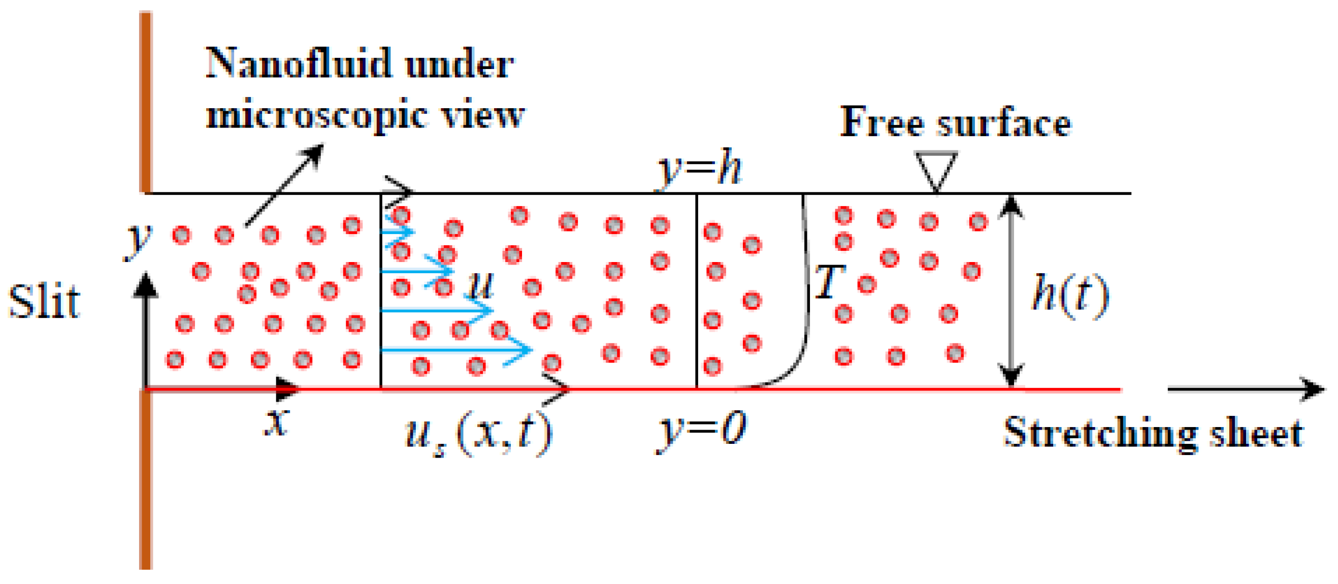
2. Flow Analysis

Over a stretched sheet, the flow of a liquid film while taking into account viscoelastic nanofluid is assessed here. Using a cartesian coordinate system, the stretchable sheet is measured along the x-axis, and the y-axis is perpendicular to the sheet. A sheet being stretched along the x-axis at a velocity of $u_s(x,t)$ is what causes the flow in a thin film of thickness $h\left(t\right)$, and it can be defined as follows [20]:

$$u_s(x,t)=\frac{bx}{1-at},$$

(1)

where both of the positive constants, a and b, have a dimension of time${}^{-1}$. Here, it is important to mention that only $t<\frac{1}{a}$ is acceptable for the current analysis. Additionally, the flow’s incompressibility is considered in a liquid thin film that is embedded in a porous medium with high porosity and permeability k because of a highly elastic sheet that emerges from a tiny slit at the origin, as shown in Figure 1. In this study, the stretching of the sheet results in a laminar motion of the nanofluid, meaning that there is no rotation velocity. Additionally, it is assumed that the nanoparticle concentration is $C_w$ at the sheet, yet it drops in the direction away from the sheet.

Further, in our research, the sheet is exposed to a variable heat flux $q_s(x,t)$ that relies on the two variables x and t in accordance with the relationship shown below [20]:

$$q_s(x,t)=-\kappa \left(\frac{\partial T}{\partial y}\right)=d{x}^2{T}_r{\left(1-at\right)}^{\frac{-5}{2}},$$

(2)

where $\kappa$ is the nanofluid thermal conductivity, d is a constant, and $T_r$ is the reference temperature. The formulation of Equation (2) acknowledges that the heat flux between the stretching sheet and the liquid film rises in proportion to $x^2$ and that it does so in a way that the heat flux grows with time. Furthermore, it is assumed that the stretched sheet receives the radiation heat flow $q_r$, which is given by [21]:

$$q_r=-\frac{4{\sigma }^{*}}{3k^{*}}\frac{\partial T^4}{\partial y},$$

(3)

where $k^{*}$ is the coefficient of absorption and ${\sigma }^{*}$ is the Stefan–Boltzmann constant. The Rosseland approximation is employed in the final equation to describe the radiative heat flux in order to avoid the nonlinear nature of the radiation term, which is a crucial point to make. Additionally, the following relation suggests that the temperature change within the flow must be extremely small in order for $T^4$ to be expanded in a Taylor series [22]:

$$T^4\cong 4T_0^{3}T-3T_0^4.$$

(4)

The essential connection between the nanofluid thermal conductivity $\kappa \left(T\right)$ and the nanofluid temperature is also taken into consideration using the relationship shown below [23]:

$$\kappa \left(T\right)={\kappa }_0\left(1+\epsilon \left(\frac{T-T_0}{T_r\frac{d{x}^2}{{(1-at)}^2}\frac{\sqrt{\frac{\nu }{b}}}{{\kappa }_0}}\right)\right),$$

(5)

where ${\kappa }_0$ is the nanofluid thermal conductivity at the slit, $\nu$ is kinematic viscosity, $T_0$ is the nanofluid temperature at the slit, and $\epsilon$ is the thermal conductivity parameter. Additionally, consideration is given to the thermophoresis phenomenon with the diffusion coefficient $D_T$ and the Brownian motion of the nanoparticles with the Brownian diffusion coefficient $D_B$ throughout the thin film layer. According to the aforementioned assumptions, the constitutive equations controlling the flow of viscoelastic fluid are as follows:

$$\nabla .\mathrm{U}̠=0,$$

(6)

which exemplifies the law of mass conservation:

$${\rho }_f\left(\frac{D\mathrm{U}̠}{Dt}\right)=\nabla .{\tau }_{ij}+\mathrm{w}̠;$$

(7)

this previous equation demonstrates the concept of conserving momentum:

$$\frac{\partial T}{\partial t}+\mathrm{U}̠.\nabla T=\nabla .\left[\left(\frac{\kappa }{{\rho }_f{c}_p}\right)\nabla T\right]-\nabla .q_r+\tau \left[(\frac{D_T}{T_0}\left({\nabla T)}^2\right)+D_B\nabla C.\nabla T\right],$$

(8)

which highlights the principle of energy conservation while accounting for the impact of thermal radiation,

$$\frac{\partial C}{\partial t}+\mathrm{U}̠.\nabla C=D_B{\nabla }^{2}C+\frac{D_T}{T_0}{\nabla }^{2}T,$$

(9)

whereas the preceding equation illustrates the conservation of nanoparticle concentration. Additionally, $\mathrm{U}̠=(u,v,0)$ is the velocity with two components u and v, and $\mathrm{w}̠=\frac{-\mu }{k}\mathrm{U}̠$ stands for the fluid’s viscoelastic Darcy impedance. Now, the momentum, concentration, and thermal energy equations in two dimensions govern the velocity, temperature, and concentration fields in the thin liquid layer take the following form ([3,23]):

$$\frac{\partial u}{\partial x}+\frac{\partial v}{\partial y}=0,$$

(10)

$$\frac{\partial u}{\partial t}+u\frac{\partial u}{\partial x}+v\frac{\partial u}{\partial y}=\nu \frac{{\partial }^{2}u}{\partial y^2}-\frac{{\alpha }_1}{{\rho }_f}\left(\frac{{\partial }^{3}u}{\partial t\partial y^2}+u\frac{{\partial }^{3}u}{\partial x\partial y^2}+\frac{\partial u}{\partial x}\frac{{\partial }^{2}u}{\partial y^2}+\frac{\partial u}{\partial y}\frac{{\partial }^{2}v}{\partial y^2}+v\frac{{\partial }^{3}u}{\partial y^3}\right)-\frac{\mu }{{\rho }_{f}k}u,$$

(11)

$$\frac{\partial T}{\partial t}+u\frac{\partial T}{\partial x}+v\frac{\partial T}{\partial y}=\frac{1}{{\rho }_f{c}_p}\frac{\partial }{\partial y}\left(\kappa \frac{\partial T}{\partial y}\right)-\frac{1}{{\rho }_f{c}_p}\frac{\partial q_r}{\partial y}+\tau \left(D_B\left(\frac{\partial C}{\partial y}\frac{\partial T}{\partial y}\right)+\left(\frac{D_T}{T_0}\right){\left(\frac{\partial T}{\partial y}\right)}^2\right),$$

(12)

$$\frac{\partial C}{\partial t}+u\frac{\partial C}{\partial x}+v\frac{\partial C}{\partial y}=D_B\frac{{\partial }^{2}C}{\partial y^2}+\left(\frac{D_T}{T_0}\right)\frac{{\partial }^{2}T}{\partial y^2},$$

(13)

where the components of velocity of the nanofluid flow are $(u,v)$, ${\rho }_f$ is the nanofluid density, ${\alpha }_1$ is the material parameter of the viscoelastic fluid, $c_p$ is the specific heat at constant pressure, $\mu$ is the viscosity, C is the nanoparticles’ concentration, $D_T$ is a thermophoretic diffusion coefficient, and $\tau$ is the heat capacity of small particles in relation to the heat capacity of basic fluids. Notably, when ${\alpha }_1=0$, our previous non-Newtonian viscoelastic model may be turned into a Newtonian model.

The following are the physical conditions for the current proposal [23]:

$$\begin{array}{c}\hfill u=u_s(x,t),v=0,-\kappa \frac{\partial T}{\partial y}=q_s(x,t),C_w=C_0-C_r\left(\frac{b{x}^2}{2\nu }\right){(1-at)}^{\frac{-3}{2}},aty=0,\end{array}$$

(14)

$$\frac{\partial u}{\partial y}=0,\frac{\partial T}{\partial y}=0,\frac{\partial C}{\partial y}=0,vs.=\frac{dh}{dt}aty=h,$$

(15)

where $C_w$ is the nanoparticle concentration along the stretching sheet, $C_0$ is the nanoparticle concentration at the slit, and $C_r$ is the reference nanoparticle concentration. Now when the situation $T_r=0$ can been excluded, let us introduce the new dimensionless variables $f,\theta$, and $\varphi$ and the similarity variable $\eta$ as follows [23]:

$$\eta =\sqrt{\frac{b}{\nu }}{\left(1-at\right)}^{\frac{-1}{2}}y,\psi =\sqrt{\nu b}{\left(1-at\right)}^{\frac{-1}{2}}xf\left(\eta \right),$$

(16)

$$\theta \left(\eta \right)=\frac{T-T_0}{T_r\frac{d{x}^2}{{(1-at)}^2}\frac{\sqrt{\frac{\nu }{b}}}{{\kappa }_0}},C=C_0-C_r\left(\frac{b{x}^2{(1-at)}^{\frac{-3}{2}}}{\nu }\right)\varphi \left(\eta \right),$$

(17)

where $\psi$ is the physical stream function that automatically achieves the mass conservation Equation (10). Additionally, as shown by the following relationships, the nanofluid velocity components u and v rely on stream function $\psi$ as:

$$u=\frac{\partial \psi }{\partial y},v=-\frac{\partial \psi }{\partial x}.$$

(18)

Now, the mathematical problem described in Equations (11)–(13) and boundary conditions (14)–(15) can be completely reduced to a collection of ordinary differential equations and the corresponding boundary conditions as below:

$$f^{{}^{\prime \prime \prime }}+f{f}^{{}^{\prime \prime }}-f^{{}^{\prime }2}-S\left(\frac{\eta }{2}{f}^{{}^{\prime \prime }}+f^{{}^{\prime }}\right)-\alpha \left[2f^{\prime }{f}^{\prime \prime \prime }+S\left(2f^{\prime \prime \prime }+\frac{\eta }{2}{f}^{\prime \prime \prime \prime }\right)-f^{\prime \prime 2}-f{f}^{\prime \prime \prime \prime }\right]-\lambda f^{{}^{\prime }}=0,$$

(19)

$$\begin{array}{c}\hfill \frac{1}{Pr}\left((1+R+\epsilon \theta ){\theta }^{\prime \prime }+\epsilon {\theta }^{\prime 2}\right)+f{\theta }^{{}^{\prime }}-2f^{{}^{\prime }}\theta -S\left(2\theta +\frac{\eta }{2}{\theta }^{{}^{\prime }}\right)+Nt{\theta }^{{}^{\prime }2}+Nb{\theta }^{{}^{\prime }}{\varphi }^{{}^{\prime }}=0,\end{array}$$

(20)

$${\varphi }^{{}^{\prime \prime }}+Sc\left(f{\varphi }^{{}^{\prime }}-2f^{{}^{\prime }}\varphi -\frac{S}{2}\left(3\varphi +\eta {\varphi }^{{}^{\prime }}\right)\right)+\frac{Nt}{Nb}{\theta }^{{}^{\prime \prime }}=0,$$

(21)

$$f\left(0\right)=0,f^{{}^{\prime }}\left(0\right)=1,{\theta }^{\prime }\left(0\right)=\frac{-1}{1+R+\epsilon \theta \left(0\right)},\varphi \left(0\right)=1,$$

(22)

$$f\left(\gamma \right)=\frac{\gamma }{2}S,f^{{}^{\prime \prime }}\left(\gamma \right)=0,{\theta }^{{}^{\prime }}\left(\gamma \right)=0,{\varphi }^{{}^{\prime }}\left(\gamma \right)=0.$$

(23)

The descriptions for each factor influencing the energy, momentum, and concentration equations are as follows:

$$S=\frac{a}{b},\alpha =\frac{{\alpha }_{1}b}{\mu (1-at)},\lambda =\frac{\mu b}{{\rho }_f(1-at)k},Pr=\frac{\mu c_p}{{\kappa }_0},R=\frac{16{\sigma }^{*}{T}_0^3}{3{\kappa }_0{k}^{*}},$$

(24)

$$Nt=\frac{d{x}^2\tau D_T{T}_r}{{\kappa }_0\sqrt{\nu b}{(1-at)}^2{T}_0},Nb=\frac{\tau D_B(C_w-C_0)}{\nu },Sc=\frac{\nu }{D_B},$$

(25)

which include the unsteadiness parameter S, the dimensionless local viscoelastic parameter $\alpha$, the local porous parameter $\lambda$, the Prandtl number Pr, the radiation parameter R, the local thermophoresis parameter $Nt$, the Brownian motion parameter $Nb$, and the Schmidt number $Sc$.

In addition, Equation (16) allows for the calculation of the parameter $\gamma$, which denotes the dimensionless film thickness as follows:

$$\gamma ={\left(\frac{b{\rho }_f}{\mu (1-at)}\right)}^{\frac{1}{2}}h\left(t\right).$$

(26)

For the entire set of governing Equations (19)–(21), it is obvious that $\gamma$ is an unknown constant that must be discovered.

3. Engineering and Industrial Quantities

The drag force expressed in terms of skin-friction coefficient $C{f}_x$, the rate of heat transfer expressed in terms of Nusselt number $N{u}_x$, and the rate of mass transfer expressed in terms of Sherwood number $S{h}_x$ are the physical parameters of the viscoelastic nanofluid flow based on the variable heat flux that are significant to industry and engineering in the processing of materials, and they are calculated in the following ways ([3,23]):

$$R{e}_x^{\frac{1}{2}}C{f}_x=-\left[f^{\prime \prime }\left(0\right)+\alpha \left(3f^{\prime }\left(0\right)f^{\prime \prime }\left(0\right)-f\left(0\right)f^{\prime \prime \prime }\left(0\right)+\frac{S}{2}\left(3f^{\prime \prime }\left(0\right)\right)\right)\right],$$

(27)

$$\left(\frac{N{u}_{x}R{e}^{\frac{-1}{2}}}{1+R}\right)=\frac{1}{\theta \left(0\right)},S{h}_{x}R{e}^{\frac{-1}{2}}=-{\varphi }^{\prime }\left(0\right),$$

(28)

where $R{e}_x=\frac{u_{s}x}{\nu }$ is the local Reynolds number. It is important to note that both the dimensionless viscoelastic parameter and the unsteadiness parameter have a direct impact on the drag force created when a viscoelastic nanofluid moves through a thin film layer.

4. Methodology

Our current physical model is governed by a highly nonlinear system of Equations (19)–(21); hence, there is no exact solution to the system. After modifying these equations from boundary-value problems to initial-value problems, through the shooting approach in MATHEMATICA software, the system can be solved numerically. Using a good initial guess, we were able to find the solution. The problem with modified initial values and initial conditions is described as follows:

$$f=J_1,f^{\prime }=J_2,f^{\prime \prime }=J_3,f^{\prime \prime \prime }=J_4,$$

(29)

$$\theta =J_5,{\theta }^{\prime }=J_6,\varphi =J_7,{\varphi }^{\prime }=J_8.$$

(30)

With the foregoing in mind, we obtain from the system of Equations (19)–(21):

$$J_1^{\prime }=J_2,$$

(31)

$$J_2^{\prime }=J_3,$$

(32)

$$J_3^{\prime }=J_4,$$

(33)

$$J_4^{\prime }=\frac{(2\alpha J_2+2\alpha S-1)J_4-J_1{J}_3-\alpha J_3^2+\lambda J_2+J_2^2+S(\frac{\eta }{2}{J}_3+J_2)}{\alpha J_1-\frac{\alpha }{2}\eta },$$

(34)

$$J_5^{\prime }=J_6,$$

(35)

$$J_6^{\prime }=\frac{Pr\left[2J_2{J}_5-\frac{\epsilon }{Pr}{J}_6^2-J_1{J}_6+S(2J_5+\frac{\eta }{2}{J}_6)-Nt{J}_6^2-Nb{J}_6{J}_8\right]}{\left(1+R+\epsilon J_5\right)},$$

(36)

$$J_7^{\prime }=J_8,$$

(37)

$$J_8^{\prime }=Sc\left(-J_1{J}_8+2J_2{J}_7+\frac{S}{2}\left(3J_7+\eta J_8\right)\right)-\frac{Nt}{Nb}{J}_6^{\prime },$$

(38)

according to the ensuing restriction requirements:

• when $\eta =0$

  $$J_1=0,J_2=1,J_6=\frac{-1}{1+R+\epsilon J_5},J_7=1,$$

  (39)
• when $\eta =\gamma$

  $$J_1=\frac{\gamma S}{2},J_3=0,J_6=0,J_8=0.$$

  (40)

Thus, the relevant boundary conditions and previously derived first-order ordinary differential equations are obtained. Among these, the condition $J_1=\frac{\gamma S}{2}$ determines the value of film thickness $\gamma$. Finally, in order to solve the aforementioned system, the shooting technique coupled with the Runge–Kutta integration approach is used.

5. Validation of the Numerical Solution

A three-point boundary value problem is represented by Equations (19)–(21), together with the boundary conditions (22) and (23). It is appropriate for numerical computation to use a reliable Runge–Kutta integrating technique. Comparing the outcomes for the drag force quantity in terms of $-f^{\prime \prime }\left(0\right)$ with those obtained by Liu et al. [21] for the Newtonian case $\alpha =0$ over an unsteady stretching sheet with various values of the unsteadiness parameter S and without the porous parameter $\lambda =0$ served as proof of the existing analysis’s efficacy and accuracy. Therefore,

Table 1. Comparison of film thickness $\gamma$ and skin friction values $-f^{{}^{\prime \prime }}\left(0\right)$ with the results of Liu et al. [21] for different values of S when $\alpha =\lambda =0$.

S	Liu et al. [21]		Present Results
	$\mathit{\gamma }$	$-{\mathit{f}}^{{}^{\prime \prime }}\left(\mathbf{0}\right)$	$\mathit{\gamma }$	$-{\mathit{f}}^{{}^{\prime \prime }}\left(\mathbf{0}\right)$
0.4	4.981454	1.134096	4.98144987	1.13409589
0.8	2.151994	1.245806	2.15199394	1.24580568
1.2	1.127781	1.279172	1.12777819	1.27917195
1.6	0.576173	1.114938	0.57616859	1.11493776

for flow characteristics includes the numerical data, along with published data of Liu et al. [21]. It seems like satisfactory agreement is reached. Following this encouraging evaluation of our numerical approach, the numerical outcomes for the non-Newtonian viscoelastic nanofluid thin-film flow model that was influenced by the variable heat flux can be discussed.

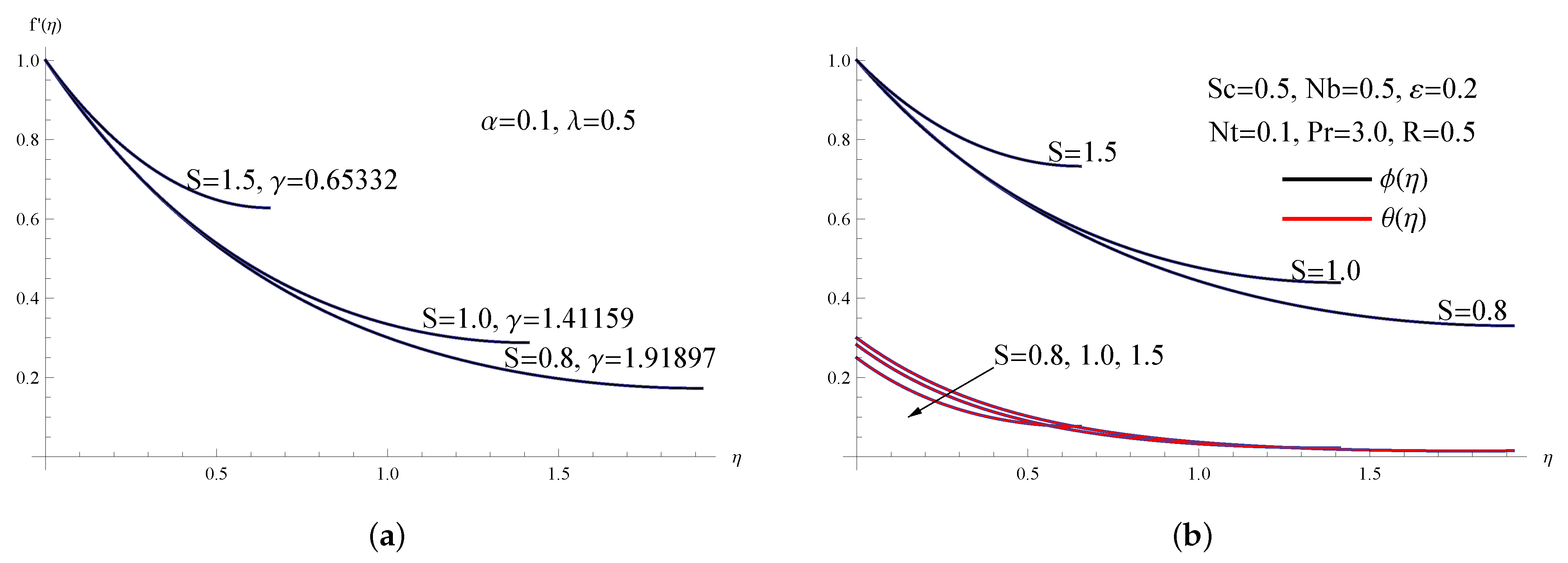
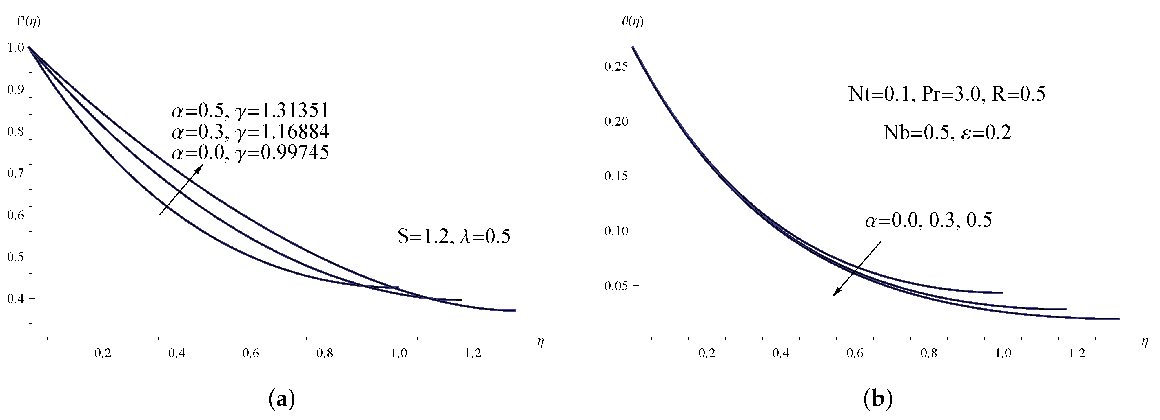
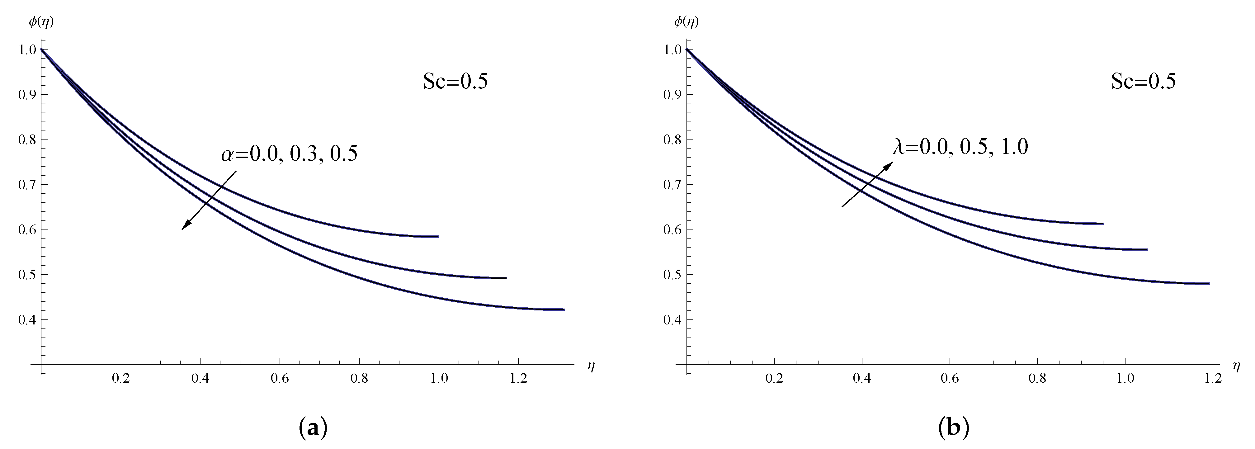
6. Interpretation of Numerical Results

The numerical outcomes and simulations from the numerical shooting method used to solve the mathematical model which described through the Equations (19)–(21), together with the conditions (22)–(23), are covered in this section. This research comprises a range of dimensionless factors whose importance is clear from the existing literature research. Regarding physical quantities, flow rate, temperature gradient, and heat mass transfer were examined along with the unsteadiness parameter S, the dimensionless viscoelastic parameter $\alpha$, the porous parameter $\lambda$, the thermal conductivity parameter $\epsilon$, the radiation parameter R, the Brownian motion parameter $Nb$, and the thermophoresis parameter $Nt$. The following ranges were used for each of the controlling physical parameters: $0.8\le S\le 1.5,$$0.0\le \alpha \le 0.5,0.0\le \lambda \le 1.0,0.0\le \epsilon \le 2.5,0.0\le R\le 2.5,0.1\le Nb\le 1.0$, and $0.0\le Nt\le 0.2$. As a result, it is possible to select the following settings for the parameters with fixed values that are employed for graphical display: $S=1.2,\alpha =0.1,\lambda =0.5,$$\epsilon =0.2,Nb=0.5$, and $Nt=0.1$. Figure 2 shows how the unsteadiness parameter S affects the profiles of temperature $\theta \left(\eta \right)$, concentration $\varphi \left(\eta \right)$, and velocity $f^{\prime }\left(\eta \right)$ in the $\eta$ direction. Firstly, the unsteadiness parameter S must range between specified values, which is the first thing we must note here. Thus, as Wang [1] pointed out, the hydromechanical thin-liquid-film problem can be solved for positive values of S in the interval $[0,2]$. Additionally, he demonstrated the reciprocity of the relationship between the unsteadiness parameter and thin film’s thickness. This relationship can be expressed as follows: as S approaches zero ($S\to 0$), the film layer thickens $\gamma \to \infty$, whereas as S approaches its maximum value of 2 ($S\to 2$), the film layer becomes extremely thin, $\gamma \to 0$. Figure 2 demonstrates that as the values of the unsteadiness parameter are increased, the velocity profile $f^{\prime }\left(\eta \right)$ and the free surface velocity $f^{\prime }\left(\gamma \right)$ rise noticeably. Additionally, it is clear that the film thickness $\gamma$ has a reversible relation of S, and as a result, the free surface velocity $f^{\prime }\left(\gamma \right)$ grows as S increases. Further, it is clear that as the unsteadiness parameter is increased, temperature profiles $\theta \left(\eta \right)$ and surface temperatures $\theta \left(0\right)$ fall, yet the thermal film thickness $\gamma$ and free surface concentration $\varphi \left(\gamma \right)$ grow in lockstep with the same parameter S. Physically, a fluid’s film thickness increases its viscosity; therefore, it is more challenging to increase the velocity of viscous non-Newtonian viscoelastic fluids because doing so would take more force to overcome the fluid’s cohesive and adhesive forces.

Figure 3 illustrates the effects of the viscoelastic parameter $\alpha$ on the velocity $f^{\prime }\left(\eta \right)$ and temperature $\theta \left(\eta \right)$ fields. The velocity distribution $f^{\prime }\left(\eta \right)$, the film thickness $\gamma$, and free surface velocity $f^{\prime }\left(\gamma \right)$ all tend to be improved by an improvement in the viscoelastic parameter’s value. Further, the temperature field $\theta \left(\eta \right)$ and free surface temperature $\theta \left(\gamma \right)$ both decline when the other parameter’s magnitude $\alpha$ rises. Mathematically, the viscoelastic parameter is inversely related to the fluid’s viscosity. Therefore, a high value of the viscoelastic parameter leads to a drop in the fluid’s viscosity, which in turn improves the fluid’s velocity through the film layer.

Figure 4 shows, for various values of the porous parameter $\lambda$, the distribution of the liquid film $\gamma$, the velocity distribution $f^{\prime }\left(\eta \right)$ inside the thin film, and the accompanying temperature distribution $\theta \left(\eta \right)$. Both the thickness of the liquid film $\gamma$ and the free surface velocity $f^{\prime }\left(\gamma \right)$ through the film layer decline when the porous parameter is raised from zero to unity. Physically, as film thickness diminishes, resistive force increases, which causes the velocity profile to diminish. Understanding and improving the performance of heat transfer is greatly influenced by the liquid film distribution over the horizontal stretching sheet. Therefore, as can be seen, the dimensionless porous parameter improved both the liquid temperature $\theta \left(\eta \right)$ and the free surface temperature $\theta \left(\gamma \right)$. Physically, the porous media in the flow model provides an obstructing force for the flow motion, which causes the fluid velocity and film thickness to diminish. Likewise, this resistance force increases the energy produced by the model, which raises the temperature distribution.

Figure 5 illustrates the features of the concentration $\varphi \left(\eta \right)$ of nanoparticles within a thin liquid film for increasing values of the dimensionless viscoelastic parameter $\alpha$ and the dimensionless porous parameter $\lambda$. Here, raising the viscoelastic parameter values result in a decrease in the concentration of nanoparticles $\varphi \left(\eta \right)$ and the free surface concentration $\varphi \left(\gamma \right)$, and the film’s thickness for the nanofluid exhibits the opposite trend. Further, both the nanoparticle concentration $\varphi \left(\eta \right)$ and the viscoelastic nanofluid’s free surface concentration $\varphi \left(\gamma \right)$ rise as the porous parameter $\lambda$ does.

Figure 6 illustrates the effects of the thermal conductivity $\epsilon$ and radiation R parameters on the temperature distribution $\theta \left(\eta \right)$ within the liquid thin film. The nanofluid temperature distribution along the sheet $\theta \left(0\right)$ and the surface temperature $\theta \left(\eta \right)$ both fall as the thermal conductivity parameter $\epsilon$ improves, but the free surface temperature $\theta \left(\gamma \right)$ exhibits a modest reversal of this trend. Furthermore, an increase in radiation parameter R causes the viscoelastic nanofluid’s free surface temperature $\theta \left(\gamma \right)$ to rise and moves the temperature distribution $\theta \left(\eta \right)$ away from the sheet. Additionally, enhancing the radiation parameter declines both the surface temperature $\theta \left(0\right)$ and the temperature distribution $\theta \left(\eta \right)$ beside the sheet.

Figure 7 emphasizes the effects of the Brownian motion parameter $Nb$ on the temperature $\theta \left(\eta \right)$ and concentration $\varphi \left(\eta \right)$ fields. According to the definition of the Brownian motion parameter, the capacity of a nanofluid to carry heat energy rises as the Brownian motion parameter does. Therefore, the result of the cumulative Brownian motion parameter is the generation of thermal energy in the thin film region. This is in accordance with the finding that, with a constant film thickness, the temperature distribution $\theta \left(\eta \right)$, the surface temperature $\theta \left(0\right)$, and the free surface temperature $\theta \left(\gamma \right)$ all rise as the Brownian motion parameter rises. Physically, a greater Brownian motion value indicates that the kinetic energy of the molecules in the nanofluid is larger, which causes more molecular collisions and shares a direct relationship with temperature. Additionally, Figure 7b shows how the same parameter $Nb$ behaves in relation to the concentration of nanoparticles $\varphi \left(\eta \right)$. The quantity of mass transferred within a liquid film region to a nanofluid medium is directly influenced by the chaotic motion of the nanoparticles. Therefore, the concentration $\varphi \left(\eta \right)$ of the nanofluid and the free surface concentration $\varphi \left(\gamma \right)$ exhibit diminishing behavior as a result of the growing value of the Brownian motion parameter. Physically, an improvement in the Brownian motion parameter describes more randomly moving nanoparticles, which causes an expansion of the temperature distribution and a contraction of the concentration profile.

Figure 8 depicts how the thermophoresis parameter $Nt$ affects the temperature $\theta \left(\eta \right)$ and concentration $\varphi \left(\eta \right)$ of nanofluids. Just because more heat energy is produced into the thin film system as a result of the thermophoresis phenomenon, the increases in temperature profiles $\theta \left(\eta \right)$ and the surface temperature $\theta \left(0\right)$ and the free surface temperature $\theta \left(\gamma \right)$ with increasing thermophoresis parameter is visible. Additionally, an increase in the thermophoresis parameter results in improvement in the distribution of nanoparticles’ concentration $\varphi \left(\eta \right)$ and the free surface concentration $\varphi \left(\gamma \right)$ of the viscoelastic nanofluid. Physically, boosting the thermophoresis parameter leads to a rise in the viscoelastic nanofluid’s thermophoretic diffusion coefficient, which raises the concentration of the nanofluid. Physically, because the thermophoresis parameter is fundamentally dependent on the heat capacity of nanoparticles, raising it will result in a wider spread of nanopaerticle concentrations.

The effects of various physical parameters on the skin-friction coefficient $R{e}_x^{\frac{1}{2}}C{f}_x$, the local Sherwood number $R{e}_x^{\frac{-1}{2}}S{h}_x$, and the local Nusselt number $R{e}_x^{\frac{-1}{2}}N{u}_x$ are now illustrated in

Table 2. Values of $R{e}_x^{\frac{1}{2}}C{f}_x$, $R{e}_x^{\frac{-1}{2}}N{u}_x$, and $R{e}_x^{\frac{-1}{2}}S{h}_x$ for various values of $S,\epsilon ,$$\alpha ,\lambda ,R,Nt$, and $Nb$ with $Pr=3$ and $Sc=0.5$.

S	$\mathit{\alpha }$	$\mathit{\lambda }$	$\mathit{\epsilon }$	R	$\mathit{Nb}$	$\mathit{Nt}$	${\mathit{Re}}_{\mathit{x}}^{\frac{1}{2}}{\mathit{Cf}}_{\mathit{x}}$	${\mathit{Re}}_{\mathit{x}}^{\frac{-1}{2}}{\mathit{Nu}}_{\mathit{x}}$	${\mathit{Re}}_{\mathit{x}}^{\frac{-1}{2}}{\mathit{Sh}}_{\mathit{x}}$
0.8	0.1	0.5	0.2	0.5	0.5	0.1	1.56398	3.339711	0.99554
1.0	0.1	0.5	0.2	0.5	0.5	0.1	1.62151	3.543831	1.01335
1.5	0.1	0.5	0.2	0.5	0.5	0.1	1.85604	4.011625	1.18829
1.2	0.0	0.5	0.2	0.5	0.5	0.1	1.43108	3.744241	0.96981
1.2	0.3	0.5	0.2	0.5	0.5	0.1	1.91377	3.755142	1.05311
1.2	0.5	0.5	0.2	0.5	0.5	0.1	2.01324	3.758601	1.10675
1.2	0.1	0.0	0.2	0.5	0.5	0.1	1.46275	3.744262	1.05908
1.2	0.1	0.5	0.2	0.5	0.5	0.1	1.65017	3.634431	0.99810
1.2	0.1	1.0	0.2	0.5	0.5	0.1	1.81997	3.774517	0.94273
1.2	0.1	0.5	0.0	0.5	0.5	0.1	1.65017	3.696661	0.99356
1.2	0.1	0.5	1.5	0.5	0.5	0.1	1.65017	4.046820	1.01457
1.2	0.1	0.5	2.5	0.5	0.5	0.1	1.65017	4.237523	1.10507
1.2	0.1	0.5	0.2	0.0	0.5	0.1	1.65017	3.749153	0.99747
1.2	0.1	0.5	0.2	1.5	0.5	0.1	1.65017	4.355022	1.02115
1.2	0.1	0.5	0.2	2.5	0.5	0.1	1.65017	4.863840	1.03684
1.2	0.1	0.5	0.2	0.5	0.1	0.1	1.65017	4.194981	0.59368
1.2	0.1	0.5	0.2	0.5	0.5	0.1	1.65017	3.634431	0.99810
1.2	0.1	0.5	0.2	0.5	1.0	0.1	1.65017	3.267371	1.04801
1.2	0.1	0.5	0.2	0.5	0.5	0.0	1.65017	3.766812	1.09521
1.2	0.1	0.5	0.2	0.5	0.5	0.1	1.65017	3.634431	0.99810
1.2	0.1	0.5	0.2	0.5	0.5	0.2	1.65017	3.559033	0.90139

below. In addition to the local Sherwood number and Nusselt number, which both measure the rate of mass transfer at the sheet surface and the rate of heat transfer, the skin-friction coefficient measures the drag force rate at the sheet surface. Evidently, the unsteadiness, viscoelastic, and porous parameters exhibit lower impedance to the drag force, which improves the skin friction. Additionally, in the presence of variable heat flux, the thermal conductivity and radiation parameters promote heat and mass transfer rates over the stretching sheet. As shown in Table 2, the values of the local Nusselt number are decreased by both the thermophoresis parameter and the Brownian motion parameter. Additionally, whilst the Brownian motion parameter increases the local Sherwood number, the thermophoresis parameter can reduce it.

7. Conclusions

Two-dimensional viscoelastic nanofluid thin-film flow induced by an unsteady stretching surface embedded in a porous medium with variable heat flux, thermal radiation, and variable thermal conductivity has been modeled numerically in this analysis. The shooting methodology is used to tackle the problem because the emergent system regulating the suggested model was exceedingly nonlinear and forced us to apply a numerical approach. Under the flow assumptions, the impacts of dimensionless factors are visually depicted. When the values of the film thickness and its corresponding skin friction values are compared, the results show good accuracy. This study has important applications in the areas of cooling, particularly in nuclear reactors, and continuous shaping. The following is a representation of the investigation’s most important findings:

• It is possible to greatly improve the nanofluid thin film’s thickness by using higher viscoelastic parameter values and lower unsteadiness and porous parameter values.
• The local skin-friction coefficient, heat transfer rate, and nanofluid temperature all increase as the porous parameter is increased, but the Sherwood number exhibits the opposite tendency.
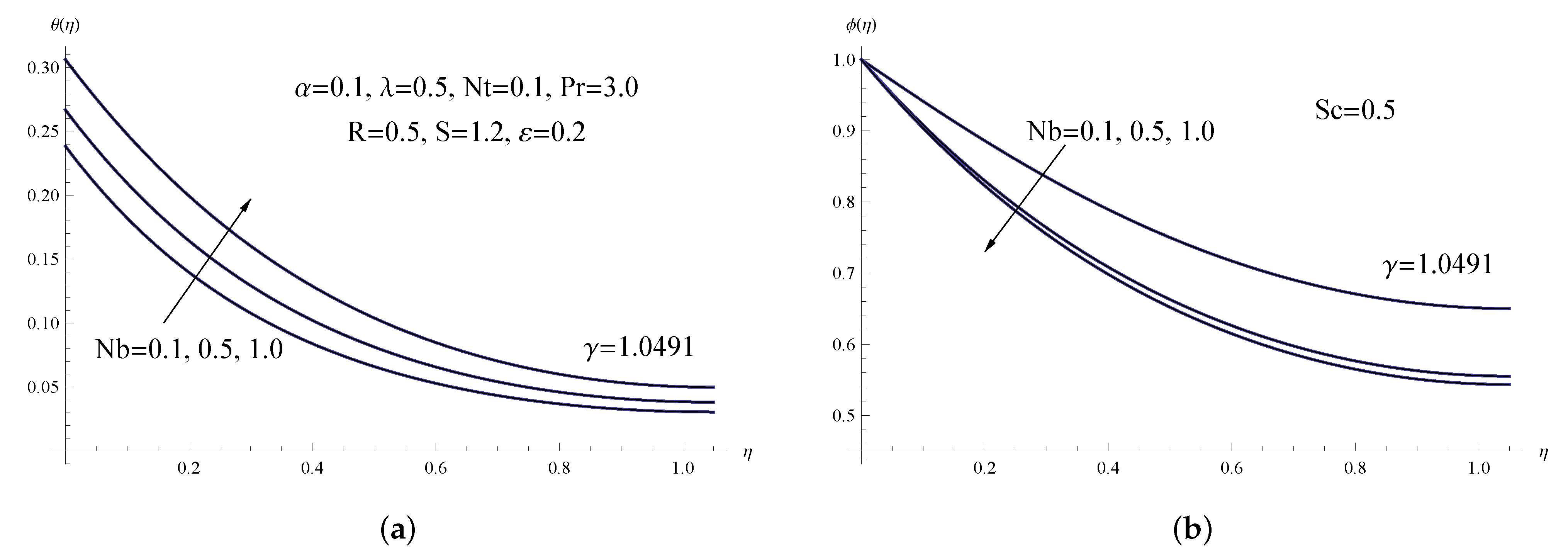
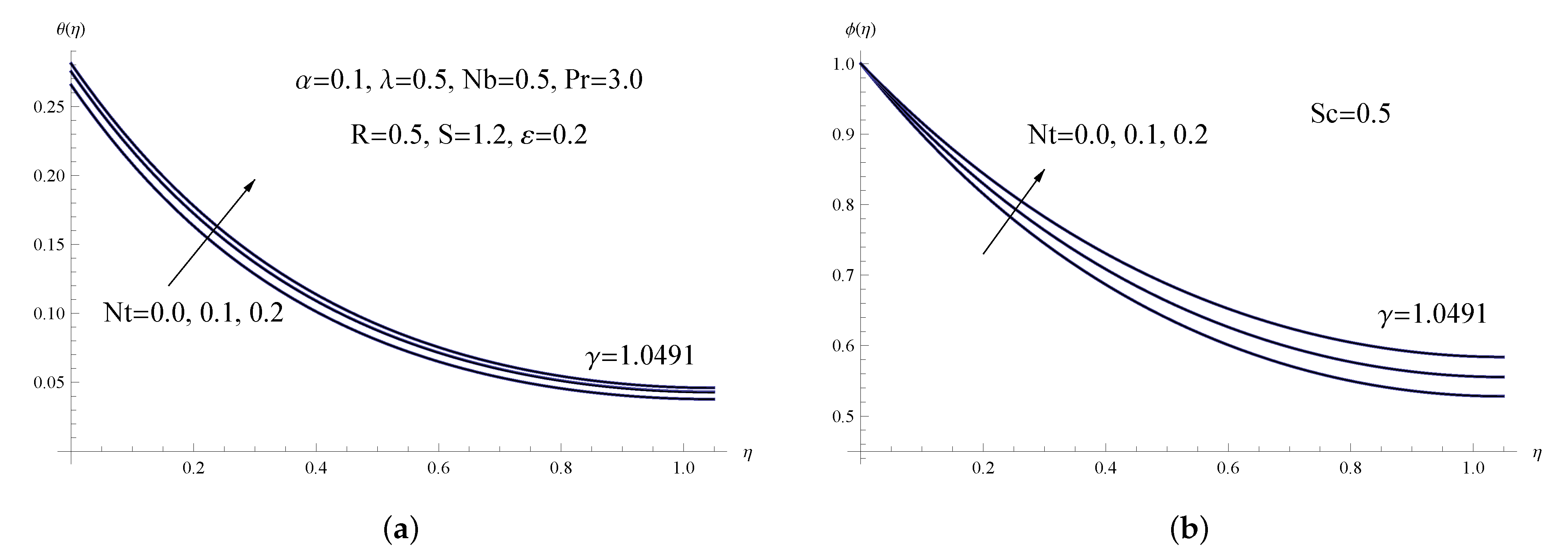
• It is feasible to successfully accomplish the best nanoparticle arrangement within the viscoelastic nanofluid liquid thin film by raising the porous parameter and the thermophoresis parameter, and decreasing the Brownian motion parameter.
• The skin-friction coefficient, the rate of surface heat transfer, and the rate of mass transfer can all be significantly enhanced by employing higher values of the unsteadiness parameter and the viscoelastic parameter.
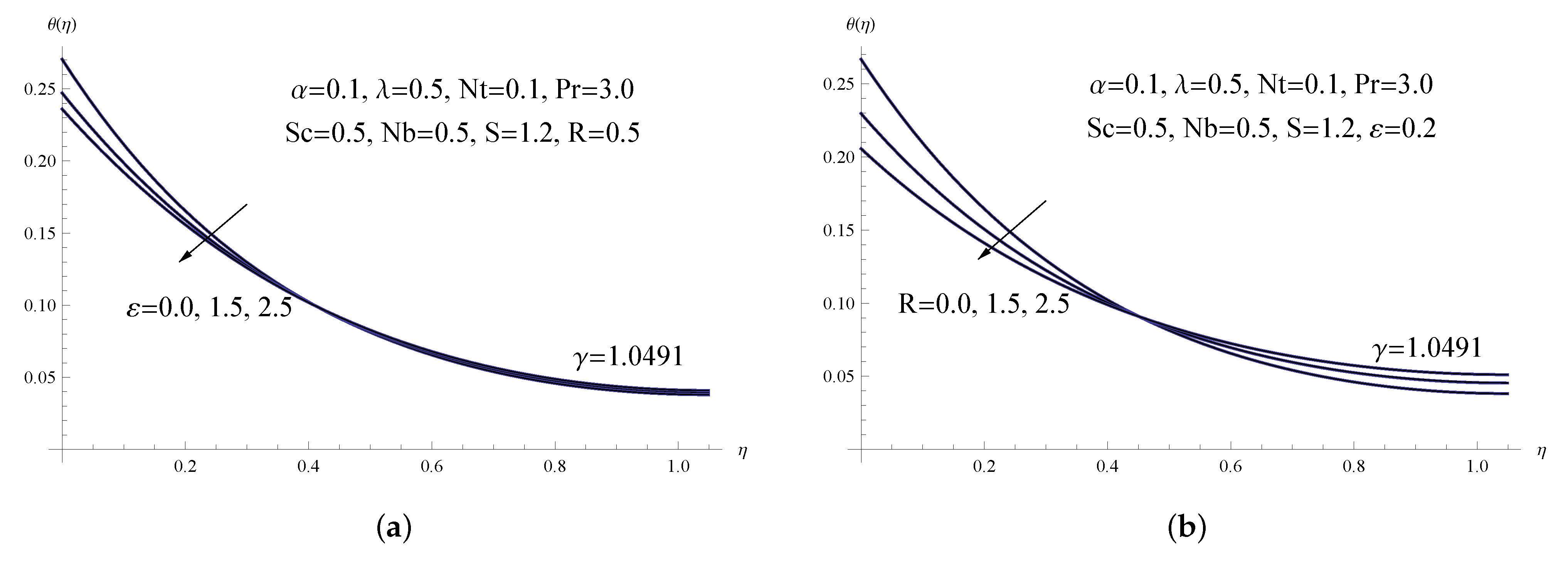
• As the thermal conductivity parameter and the thermal radiation increase, the temperature distribution and sheet temperature are both reduced.
• Improvements in the thermal conductivity and radiation parameters cause the local Nusselt and Sherwood numbers to rise, but increases in the thermophoresis parameter cause the former two to decrease.
• It is possible to use this kind of problem to enhance the industrial technology’s mass and heat-transmission mechanism.
• In the future, we intend to expand on this research by analyzing how variable mass flux and variable density affect the flow properties through porous media regulated by the modified Darcy law.

References

- Andersson, H.I.; Aarseth, J.B.; Braud, N.; Dandapat, B.S. Flow of a power-law fluid film on an unsteady stretching surface. J. Non-Newtonian Fluid Mech. 1996, 62, 1–8. [Google Scholar] [CrossRef]
- Wang, C.; Pop, I. Analysis of the flow of a power-law fluid film on an unsteady stretching surface by means of homotopy analysis method. J. Non-Newtonian Fluid Mech. 2006, 138, 161–172. [Google Scholar] [CrossRef]
- Abbas, Z.; Hayat, T.; Sajid, M.; Asghar, S. Unsteady flow of a second grade fluid film over an unsteady stretching sheet. Math. Comput. Model. 2008, 48, 518–526. [Google Scholar] [CrossRef]
- Wang, C.Y. Liquid film on an unsteady stretching surface. Q. Appl. Math. 1990, 48, 601–610. [Google Scholar] [CrossRef] [Green Version]
- Choi, U.S. Enhancing thermal conductivity of fluids with nanoparticles. ASME FED 1995, 231, 99–103. [Google Scholar]
- Buongiorno, J. Convective transport in nanofluids. ASME J. Heat Mass Transf. 2006, 128, 240–250. [Google Scholar] [CrossRef]
- Ramzan, M.; Bilal, M.; Chung, J.D.; Farooq, U. Mixed convective flow of Maxwell nanofluid past a porous vertical stretched surface—An optimal solution. Results Phys. 2016, 6, 1072–1079. [Google Scholar] [CrossRef] [Green Version]
- Khan, M.; Azam, M.; Alshomrani, A.S. On unsteady heat and mass transfer in Carreau nanofluid flow over expanding or contracting cylinder with convective surface conditions. J. Mol. Liq. 2017, 231, 474–484. [Google Scholar] [CrossRef]
- Sharma, K.; Gupta, S. Viscous dissipation and thermal radiation effects in MHD flow of Jeffrey nanofluid through impermeable surface with heat generation/absorption. Nonlinear Eng. 2017, 6, 153–166. [Google Scholar] [CrossRef]
- Patel, H.R.; Mittal, A.S.; Darji, R.R. MHD flow of micropolar nanofluid over a stretching/shrinking sheet considering radiation. Int. Commun. Heat Mass Transf. 2019, 108, 104322. [Google Scholar] [CrossRef]
- Alali, E.; Megahed, A.M. MHD dissipative Casson nanofluid liquid film flow due to an unsteady stretching sheet with radiation influence and slip velocity phenomenon. Nanotechnol. Rev. 2022, 11, 463–472. [Google Scholar] [CrossRef]
- Yousef, N.S.; Megahed, A.M.; Ghoneim, N.I.; Elsafi, M.; Fares, E. Chemical reaction impact on MHD dissipative Casson-Williamson nanofluid flow over a slippery stretching sheet through porous medium. Alex. Eng. J. 2022, 61, 10161–10170. [Google Scholar] [CrossRef]
- Areshi, M.; Alrihieli, H.; Alali, E.; Megahed, A.M. Temperature distribution in the flow of a viscous incompressible non-Newtonian Williamson nanofluid saturated by gyrotactic microorganisms. Mathematics 2022, 10, 1256. [Google Scholar] [CrossRef]
- Lund, L.A.; Omar, Z.; Dero, S.; Khan, I.; Baleanu, D.; Nisar, K.S. Magnetized Flow of Cu + Al2O3 + H2O Hybrid Nanofluid in Porous Medium: Analysis of Duality and Stability. Symmetry 2020, 12, 1513. [Google Scholar] [CrossRef]
- Alrehili, M. Development for cooling operations through a model of nanofluid flow with variable heat flux and thermal radiation. Processes 2022, 10, 2650. [Google Scholar] [CrossRef]
- Alrihieli, H.; Alrehili, M.; Megahed, A.M. Radiative MHD nanofluid flow due to a linearly stretching sheet with convective heating and viscous dissipation. Mathematics 2022, 10, 4743. [Google Scholar] [CrossRef]
- Farooq, M.; Khan, M.I.; Waqas, M.; Hayat, T.; Alsaedi, A.; Khan, M.I. MHD stagnation point flow of viscoelastic nanofluid with non-linear radiation effects. J. Mol. Liq. 2016, 221, 1097–1103. [Google Scholar] [CrossRef]
- Hayat, T.; Waqas, M.; Shehzad, S.A.; Alsaedi, A. Mixed convection flow of viscoelastic nanofluid by a cylinder with variable thermal conductivity and heat source/sink. Int. J. Numer. Methods Heat Fluid Flow 2016, 26, 214–234. [Google Scholar] [CrossRef]
- Macha, M.; Kishan, N. Boundary layer flow of viscoelastic nanofluid over a wedge in the presence of buoyancy force effects. Comput. Therm. Sci. Int. J. 2017, 9, 257–267. [Google Scholar]
- Liu, I.-C.; Megahed, A.M.; Wang, H.-H. Heat transfer in a liquid film due to an unsteady stretching surface with variable heat flux. ASME J. Appl. Mech. 2013, 80, 041003. [Google Scholar] [CrossRef]
- Liu, I.-C.; Wang, H.-H.; Umavathi, J.C. Effect of viscous dissipation, internai heat source/sink, and thermal radiation on a hydromagnetic liquid fiim over an unsteady stretching sheet. J. Heat Transf. 2013, 135, 031701. [Google Scholar] [CrossRef]
- Megahed, A.M. Flow and heat transfer of a non-Newtonian power-law fluid over a non-linearly stretching vertical surface with heat flux and thermal radiation. Meccanica 2015, 50, 1693–1700. [Google Scholar] [CrossRef]
- Nourhan, I.G.; Megahed, A.M. Hydromagnetic nanofluid film flow over a stretching sheet with prescribed heat flux and viscous dissipation. Fluid Dyn. Mater. Process. 2022, 18, 1373–1388. [Google Scholar]