Abstract
The increase in energy costs has led researchers and practitioners to investigate the energy consumption of buildings and propose solutions for its improvement. This research aimed at estimating the effect of different temperature control strategies on the energy consumption of a building. This study belongs to the field of research that considers both the structural characteristics and the conditioning systems incorporated into the design or renovation of buildings. The objective was to identify the optimal settings that led to the maximization of energy performance under intermittent occupancy considering the building’s structural and conditioning system characteristics and environmental conditions. To reach this objective, it was necessary to use simulation software that considered all these characteristics simultaneously in a dynamic environment. Specifically, the effect of the geometric and structural characteristics on the thermal profile of the building was investigated by implementing a dynamic hourly regime with temperature fluctuations around an assigned set-point. The study showed that for models with heavy masonry walls, the annual thermal dispersion of the hourly regime was much lower than for the corresponding models with light masonry walls. These results and the related method could be considered by researchers and practitioners for the design and/or renovation of buildings.
1. Introduction
This paper aimed to elucidate, through the collection and processing of data provided by computational simulations, how a building’s temperature control strategy affects its energy performance and identify how this strategy can minimize the demand for energy. In addition, the effect of the geometric and structural characteristics on the thermal requirements of a building was explored by implementing a dynamic hourly regime involving temperature fluctuations. Our objective was to consider both the structural characteristics and conditioning systems of buildings in order to define optimal configurations and system management strategies for specific environmental conditions. In order to achieve this goal, we used a numerical simulation method.
The tests were conducted in two phases: the first part of the study aimed to identify the geometric, structural, and plant-engineering factors that most strongly influenced the energy performance of the modeled buildings. In the second phase, we analyzed the effect of the system settings, i.e., the varying hourly temperature set-points, on the energy performance.
Considering that 44% of all energy used is consumed by buildings in the domestic, tertiary, or industrial sectors, and that buildings are responsible for 36% of CO2 emissions [1], it is fundamental to study and design more efficient heating systems in order to minimize buildings’ energy consumption. To achieve this, different computer simulation methods [2,3] have been developed to analyze buildings’ energy performance. Computer simulations were used to investigate the reduction in energy consumption achieved via the conditioning of tertiary-sector buildings in tropical zones [4]: the simulation analysis defined some energy efficiency strategies. Computational studies were carried out by taking into account the temperature fields of the airspace for three types of heating systems using the ANSYS Fluent software package (version 2021R2) [5]. The results facilitated the choice of more appropriate building heating systems. In [6], an overview of the theory and assumptions underlying building simulation software was presented, while in [7], selection criteria based on the energy user’s needs were proposed. More than one hundred simulation software packages were reviewed in [8], which concluded that none were applicable to analyzing all types of residential energy-management systems. Clarke and Hensen [9] underlined that simulations tools are limited, and that no single development organisation possesses the necessary expertise in all areas. As part of their work, the authors explained the characteristics of the simulation software selected to achieve the study objectives, with the aim of considering both the building’s structural characteristics and conditioning systems and the settings of the heating system.
In [10], the authors focused their attention on six topics: ventilation performance prediction, whole-building energy and thermal load simulation, lighting and daylight modeling, building information modeling, indoor acoustic simulation, and the lifecycle analysis of buildings. By studying the evolution of building simulation software from 1987, they suggested that, given the complexity of buildings in terms of the integration of components and systems, simulations should be able to provide holistic data for decision making. In [11], the authors used the FEM technique to simulate the behaviour of a ceramic slab as an external coating. According to their simulation results, the heat loss decreased by 42% with respect to a traditional wall without any thermal insulator installed. Barone et al. [12] compared the results of a simulation model with measurements obtained from a real test room. They showed that the simulated indoor air and surface room temperatures were similar to the corresponding experimental data (the differences were between 0.5 °C and 1 °C). In [13], the authors reviewed the current trends in simulation-based building performance optimization (BPO) and defined major criteria for tool selection and evaluation. They underlined a breakthrough in using evolutionary algorithms to solve highly constrained envelope, HVAC, and renewable optimization problems. Waltz [14] examined building energy simulation processes by describing the data needed to build a model, define a simulation model, evaluate the results, and validate the results in respect to reality. In [15], the authors provided guidance for building design professionals when selecting the most appropriate tool by underlining important evaluation parameters such as cost, training, design tool complexity, and validation.
In this work, we used the simulation software “EC700—Calculation of energy performance of buildings” released by the Italian software company Edilclima S.r.l. (Brescia, Italy), which allowed us to analyze the case study considered. The novelty of this study lies in the determination of a temperature control strategy by considering a building’s structure, conditioning system characteristics, and environmental characteristics. The proposed method could be considered for building design and/or renovation in order to maximize energy performance.
This work is structured as follows. After this introduction, Section 2 explains how the applied software functions. Section 3 describes the building characteristics and the case under consideration, presenting the energy models and dataset extrapolated following the simulations. In the Section 4, after presenting the results of the first simulation, we optimize the scenarios by defining the correct set of variables to be applied in the simulations. In Section 5, we analyze the results obtained through the computations, and in the last section, a critical judgment is presented for each scenario.
2. Problem and Simulation Software Characteristics
In order to evaluate how the setting of a building’s heating system affects its energy performance, we developed a realistic case study by creating energy models of a building using simulation software dedicated to calculating the energy performance of buildings. The software was used to simulate various scenarios and to extrapolate the results for subsequent re-elaboration and critical analysis. We selected this instrument because it complies with the UNI/TS 11,300 technical specifications and, moreover, because it offered the possibility of carrying out simulations in a dynamic hourly regime.
For the modeling of a typical building, both the envelope and all the parts of the heating system (generation, distribution, setting, and emission) were taken into consideration. Numerous parameters are needed to define the characteristics of a building. In this study, we evaluated the effect that some of these variables, considered significant, had on energy performance: (1) the thermal inertia of the building, represented by the recovery factors based on the mass of the building itself; and (2) the size of the heat generator, based on the thermal power required by the building.
Three values were chosen for each variable, thus generating nine possible combinations and as many energy models. The specifications are shown in Table 1 and Table 2.

Table 1.
Values of selected variables.
Table 2.
Codes for the study models obtained by combining the values of the chosen variables.
The software used to run the simulations was released by the Italian software company Edilclima S.r.l., representing a module that was part of a larger package of applications in the field of thermotechnical design. The software was “EC700—Calculation of energy performance of buildings”, which was equipped with a graphical interface and, through a single data input, allowed the following calculations to be made:
- Energy performance of the building under an hourly dynamic regime, according to the UNI EN 52016-1 standard;
- Winter power, for sizing the heating system and correctly calculating yields, according to the UNI EN 12831 standard;
- Useful winter and summer energy, for the evaluation of the building’s thermal performance, according to the UNI/TS 11300-1 technical specification;
- Primary energy for heating services, domestic hot water production, ventilation, and lighting, according to the UNI/TS 11300-2 and UNI/TS 11300-4 technical specifications;
- Primary energy for cooling, according to the UNI/TS 11300-3 technical specification;
- Primary energy for the transport of people or things (lifts, escalators, moving walks), according to the UNI/TS 11300-6 technical specification;
- The evaluation of the contributions provided by renewable-source plants (solar thermal, solar photovoltaic), according to the UNI/TS 11300-4 technical specification.
The advantage of this simulation software was the introduction of an hourly dynamic calculation method for building energy performance, in compliance with the UNI EN ISO 52016-1:2018 standard. This calculation methodology allowed a more precise and accurate assessment of the energy needs of the building, taking into account, for example, the real management and use profiles of the building. The software was provided with an archive of hourly climatic data, including, for each Italian municipality, the hourly values of external temperature, direct and diffuse solar irradiance, external relative humidity, vapor pressure, and average wind speed. Moreover, it was possible to load punctual data (e.g., hourly data relating to the external air temperature, relative humidity, solar radiation, wind speed and direction, and amount of precipitation) for the desired area and carry out relevant simulations.
The definition of hourly use profiles (for both residential and non-residential buildings) was facilitated by the presence of archives integrated into the software, which allowed us to recall pre-compiled standard profiles. The hourly calculation of the shading was carried out automatically by the software, which superimposed the profile of the shadows caused by external elements, balconies, nearby buildings, etc., on the solar path diagram.
The qualifying element of the software was the in-depth analysis of the calculation results (see Appendix A), which allowed us to evaluate:
- The correct sizing of the heating system according to the use and occupation profiles of the building;
- The comfort/discomfort hours of the internal conditions (in the event, for example, of system under-sizing, being unable to satisfy the requirements of the set-point temperatures);
- The maximum internal summer temperature that can be reached in the building in the absence of the cooling system (“free floating” calculation).
Finally, it was possible to partially calculate various factors, such as the heat exchange from transmission through opaque structures, windows, and thermal bridges; the free internal contributions; the contributions due to solar radiation through windows and opaque structures; and the heat exchange from extra-flow and ventilation. Another strength of the software was the detailed and articulated modeling of plant subsystems, allowing management of any type: for example, centralized or autonomous heating and cooling and domestic hot water systems in any combination.
Moreover, the software calculated the generation losses (traditional and condensing boilers, modulating or not) in compliance with the UNI/TS 11300-2 technical specification.
3. Building Characteristics and Case Study
The simulations began with the creation of a building model as a reference. Specifically, we chose a building that could be used as offices.
First of all, the building envelope was created by defining its structural components and geometry. The building comprised a single above-ground level; it had a square plan of 10 m per side and a net internal height of 3 m. Inside, there were several rooms separated by partitions of plastered brick blocks, closed in by brick–cement floors. Furthermore, four types of windows were added, all with metal frames and double glazing, equally distributed along the perimeter; the blinds were light-colored internal shutters. Regarding the plant engineering, only components relating to a winter air-conditioning system were implemented. The building was served by a single generator, i.e., a modulating condensing boiler with variable nominal power, which distributed the heat transfer fluid (water) between the room terminals, i.e., radiators without thermostatic valves. Environmental setting was carried out via a zone chrono-thermostat and a climatic sonde directly interfaced with the heat generator.
3.1. General Data
Firstly, the data relating to the project were requested, such as the master data of the building in question, the intended use, the purpose of the calculation, and the desire to make additional calculations beyond the standard ones. With regard to the latter choice, during the operational phase, we opted to conduct the analysis using the dynamic hourly calculation method according to the UNI EN ISO 52016 standard, as this represented the object of the present study.
The entries relating to any clients and professionals were not taken into account; in any case, the data required by the program were the same for each professional field, which had no effect on the purposes of the calculation procedure and the expected results. In this software, it was possible to choose how the building was described through an identification code related to the chosen combination of variables, the intended use coinciding with the category “E.2—Buildings used as offices and similar”. Energy diagnosis was selected as the purpose of the calculation, because this was the option compatible with the dynamic hourly procedure.
Subsequently, monthly and hourly climatic data were requested, but, as mentioned above, the software had an archive containing these codified values for each Italian municipality; therefore, once the location of the building had been defined, this information was automatically input (see Appendix B).
We proceeded with a section relating to the regulatory regime, including legal checks that depended on the chosen Italian region and may provide for the adoption of national settings or more stringent regional settings. Specifically, having chosen to locate the theoretical study building in Lombardy, DDUO 18.12.19 n. 18546 applied for the legal checks and the technical report, while decree 30.07.15 n. 6480 (CENED + 2.0) applied as regards energy certificates.
Lastly, default values referring to the construction and energy aspects of the building had to be set, including some relating to the rooms and areas that were subsequently defined, though theses vales could be changed in subsequent steps if necessary. The software automatically proposed some of these values based on the intended use of the building previously chosen.
We chose to include the recommended values for all the items, except for those relating to the mass and thermal inertia of the building, which were the subject of this case study and therefore among the variable parameters identified for the simulations (A), as described in Table 3.
Table 3.
Codes for the study models obtained by combining the values of the chosen variables.
3.2. Building Envelope
After defining the first general input data, we proceeded with the definition of the building envelope components and all the structures that would then identify the potential dispersing surfaces and the air-conditioned volumes.
The elements were divided into five main categories:
- Walls: vertical opaque dispersing elements with a horizontal flow, such as masonry, doors, and boxes for the shutters of the windows;
- Floors: horizontal dispersing elements with a descending flow;
- Ceilings: horizontal dispersing elements with an upward flow, i.e., the floors above rooms, such as ceilings and both flat and sloping roofs;
- Thermal bridges: areas of the envelope with linear dispersion formed due to geometric or material inhomogeneity between the building elements;
- Windowed components: all transparent surfaces, whether vertical, such as windows, or horizontal, such as skylights.
For all these elements, it was necessary to provide the appropriate stratigraphy and thermal characteristics, such as the typology of the environments between which they were interposed, thus defining the specific transmittance properties that conditioned the energy flow of thermal dispersion. For the choice of the constituent elements, it was necessary to maintain several constant characteristics in order to avoid distorting the experiment, such as the surface thermal transmittance of the entire technological package and its thickness. If the latter was to change, certain geometric factors of the building would vary from case to case, such as, for example, the calculation of the dispersing surfaces and the gross volume.
In the following section, we will explain in detail how this last assumption did not remain constant but underwent changes due to requirements that emerged during the analysis of the data collected from the processed simulations.
3.3. Shading
The dynamic hourly calculation provided for the possibility of expressing hourly opening and closing profiles for the blackout elements and curtains, so as to decrease or increase the solar energy contribution to the building system. The input was extremely precise, as it allowed us to create periods of flexible length and to choose the orientation of any closed shadings hour by hour.
3.4. Geometric Characteristics
The geometric characteristics of the building were defined first by drawing the wall elements using CAD, so as to arrange the architectural plans, and then by inserting the components such as windows and doors. For each floor, it was possible to define default properties that could then be modified independently for each building component or for each air-conditioned room.
It was possible to associate thermal bridges with each masonry element, which could be created using the ceiling or the floor via the default values of the floor or by assigning them in a targeted manner by flow direction.
For the correct calculation, it was necessary to define the building’s zoning by identifying the different climatic zones, i.e., the volumes governed by their own zone thermostat and the individual rooms. The definition of the zones included data relating to the intended use, the mass of the building, the lighting, and the hourly climate profile. The latter allowed us to precisely control each day by assigning temperature and humidity set-point values for winter and summer air conditioning; thus we could alternate full-load periods with periods of attenuation or shutdown in the system.
The recreated models had a variable number of floors, which, for simplicity of construction, were all identical to one defined by default and characterized by a square plan with a courtyard placed in a barycentric position, a net height of 3.0 m, and rooms consistent with the choice made previously relating to the intended use of the building. Furthermore, an independent thermal zone was assigned to each floor. It was also possible to manage each room by assigning it to the appropriate climatic zone, defining the seasonal set-point temperatures, and choosing the calculation method for ventilation; the latter directly influenced the value of energy losses. It was possible to assign the default data of the floor to the rooms or set the type of floor and ceiling in a targeted manner; these could be dispersing or non-dispersing opaque horizontal surfaces according to the neighbouring environment with which they interfaced.
A simple three-dimensional model of the simulation shell displayed via the graphical user interface is presented in Figure 1.
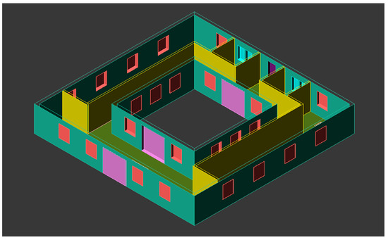
Figure 1.
Three-dimensional model of the simulation shell.
Finally, it was possible to construct the volumes of the fixed shadings, such as the overhangs belonging to the building itself (balconies, overhanging roofs, pillars, etc.); nearby buildings; and trees. For the vegetation component, it was also possible to define the monthly presence profile of the leaves, so as to modify the blockage of solar radiation that they were able to provide during the year.
3.5. Air-Conditioned Areas and Rooms
This phase of the definition of the building system took on a more informative than operational meaning as it had the purpose of showing the results of exporting the graphic input and summarizing the characteristics of each zone and room. Among the most interesting outputs were the data relating to the surfaces and volumes of the building, calculated as both net and gross; of these, the surface/volume ratio stood out, describing the gross external surface (without N-type structures) and the gross volume. N-type structures are building elements that divide two air-conditioned rooms belonging to the same thermal zone; therefore, they do not define an energy dispersion surface.
3.6. Service Plants
Having completed the modeling part of the envelope, the plant components were sized. The energy services implemented were:
- Heating: the possibility of setting up a single centralized system that served all the air-conditioned areas, or an independent one with exclusive circuits and generators for each area;
- Mechanical ventilation;
- Domestic hot water: the possibility of producing hot water using the same generator that supplies the heating, or autonomously with a dedicated generator;
- Cooling: as for the heating service, it could be centralized or autonomous;
- Renewable sources: divided into solar thermal, for the production of DHW (domestic hot water) and/or heating, and solar photovoltaic, for the production of electricity.
Once the general configurations of the energy services were defined, it was possible to determine the dimensions of the relative systems.
For the purposes of this study, only the sizing of the heating system is shown. We defined the general data of the circuits, such as the monthly activation times, which in the case of an hourly dynamic study with selected intermittence profiles should be set according to the temperature profile from the set-point, and any corrective factors.
The software offered default values that could be modified based on various parameters, such as the type of heat transfer fluid (air or water) and the type of terminals installed in the room.
Once the creation of the circuits was completed, the heat generators were defined, whose activation could take place on an hourly basis with priority or as a supplement for generators playing the main role. Each type of generator required data relating to the power supplied, the yields, the energy source consumed, and the electrical power absorbed by the accessory components.
Once the generator profile was completed, the operating regime was defined, with the possibility of setting time bands for attenuation or shutdown.
4. Optimization of the Scenario Variables
As briefly mentioned above, the first experimental simulations were conducted on the nine potentially implementable models identified by considering the two variable characteristics (Table 2). Each building model was calculated by setting an operating regime for the heating system according to the energy required based on the assumed hourly set-point temperatures. With the intention of performing a direct comparison with consistency in the data, the definition of the set-points was kept identical for each model, i.e., operation at 20 °C from 07:00 to 19:00 and attenuation in the hours 00:00–7:00 and 19:00–24:00. The criterion chosen for the comparison of the results was based on the reconstruction of a representative curve of the annual energy supplied by the generator as the attenuation temperature varied in the climatic zones. The following nomenclature was used:
- Tatt is the attenuation temperature in each case.
- Tset-point is the objective fixed temperature.
- QH,gen,out is the absolute value of the energy input associated with the operation of the generator, where QH,gen,out,max is the maximum value of the energy input, and QH,gen,out,min is the minimum value of the energy input.
We proceeded by defining, for each model, a series of points identified within a graph showing:
- On the abscissa, in ascending order, the values of the ratio between the attenuation temperature in each case (Tatt) and the temperature (Tset-point) fixed at 20 °C;
- On the ordinate, the absolute value of the energy input (QH,gen,out).
The following graph (Figure 2) shows the comparison between models A1.B1, A2.B1, and A3.B1, with the aim of demonstrating the low relevance of the parameters that reduced the variable A2.
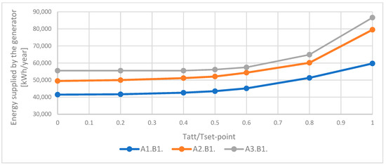
Figure 2.
Comparison of annual energy input of the generator, with set-point 12/24, as the attenuation temperature varied.
In the case of a building with an average mass, both the progression of values and the absolute energy input were moderate in comparison to the results for light and heavy buildings (A1 and A3). For greater synthesis, the other comparative analyses relating to the mass variation of the building with “large” and “huge” generators are not reported, since the behavior was completely analogous to the results of the previous comparison. The results obtained from the analysis with inverted factors, i.e., by comparing the graphs of buildings with a constant mass and variable generator size, were identical. The comparative graphs are not shown, because they were not significant for the experiment. Following these considerations, and in order to simplify the simulation scenarios, the process of investigating the dependence of the building’s energy performance on defined variables continued by eliminating the characteristic values A2 and B2, as they were considered to be of little significance. At this point, since the combinations for the energy models were reduced to four, due to the elimination of some of the values chosen for the variables A and B, we decided to make substantial changes to the models that remained in play.
4.1. Primary Energy Results
The first change adopted arose following the analysis of all the curves on the graph Tatt⁄Tset-point—QH,gen,out. Initially, we expected to obtain progressions that highlighted five distinct phases:
- A maximum energy delivery phase corresponding to the case with Tatt⁄Tset-point =1, i.e., when the thermal zone was set with a temperature of 20 °C 24 h a day for every day of the year;
- A descent phase, during which there was a decrease in the energy supplied as a function of the decrease in the Tatt⁄Tset-point ratio;
- The possibility of finding a minimum value of energy produced by the boiler, which varied from one energy model to another;
- A phase of rising consumption following the further decrease in the Tatt⁄Tset-point value beyond the value found in phase 3;
- A new maximum corresponding to Tatt⁄Tset-point = 0, i.e., when the attenuation temperature was set to its minimum value of 0 °C.
This result was expected especially for high-mass buildings, because they have a high thermal inertia; unfortunately, in no case did this theoretical behavior appear. The graph obtained experimentally turned out to be a curve with a pseudo-exponential trend showing maximum consumption at Tatt⁄Tset-point = 1, followed by a constant decrease in energy towards an asymptotic value.
With the intention of making progress in the analysis of the models and the related energy expenditure, it was later decided to introduce an additional time combination which envisaged setting the Tset-point at 20 °C for only 4 h a day, during the hours 09:00–13:00, as a contrast to the 12 h operation; therefore, in the latter case, the remaining 8 h were managed in attenuation. Thanks to the addition of this new scenario, the graph used up to now for the analyses took on greater importance, because it allowed us to evaluate the influence of the heating system settings on the single energy model. Figure 3 represents the comparison for energy model A3.B3, i.e., the building with heavy masonry and a “huge” radiator.
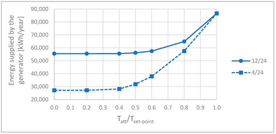
Figure 3.
Comparison of the annual energy input of the generator for building A3.B3 with set-points 12/24 and 4/24 as the attenuation temperature varied.
4.2. Light Masonry and Heavy Masonry
The second variation implemented on the models arose from the constant search for the theorized behavior of the energy curve supplied by the generator as the ratio Tatt⁄Tset-point varied. At this point, the focus shifted to the assumptions previously made regarding the characteristics of the perimeter walls, such as the stratigraphy, which directly affected the surface mass and surface transmittance. With regard to these last two parameters, we worked with the intention of making the gap, in terms of mass, between the walls defined as light and those defined as heavy as evident as possible, while keeping the thermal transmittance as constant as possible to maintain the homogeneity of the comparison. We therefore decided to modify the models by combining variable A1 with masonry stratigraphically composed of a single 30 cm perforated brick element with both internal and external plastering; for the A3 variable, instead of the perforated block, we implemented natural stone with a thickness of 100 cm. An insulator was positioned externally to both structures to control the transmittance, thus bringing it to a value close to 0.23 W⁄(m2 K). This modification of the composition of the structures and, consequently, their thickness caused some assumptions made during the creation of the first energy models to change: some geometric characteristics were no longer identical when parameter “A” varied, such as the S:V ratio, which was totally dependent on the gross external surface area and gross volume.
As mentioned above, the decision to make these changes was aimed at finding a curve closest to what was theorized regarding the trend of the energy supplied by the generator as the ratio Tatt⁄Tset-point varied. Furthermore, the same comparison graphs should have shown greater differences, as the impact of the building’s thermal inertia on its energy performance increased. Continuing with exploration of the influence of the mass of the building on the loads required by the generator, an attempt was made to further accentuate the difference between heavy and light masonry by removing the insulating layer placed on the external profile. This decision stemmed from the desire to entirely attribute the thermal capacity of the element to the structural component alone, thus eliminating the contribution of the insulating material.
For this last step, a third variable was introduced, effectively making it possible to implement new combinations for the creation of further energy models to be compared. The new discriminant was therefore the presence or absence of the insulating layer outside the perimeter walls, which, if present, was marked by the letter “I” and, if absent, by the letter “N”. Naturally, attention was paid to the transmittance value of the masonry components, guaranteeing a uniform value even after the insulation had been removed.
4.3. Minimum Radiators and Huge Radiators
The last variable introduced, in chronological order, was the result of further analyses of the results obtained from the simulations, i.e., the power peaks supplied by the generator on a monthly basis. Attention was focused on these graphs as it was noted that, in all cases, the maximum power value generated in the months from October/November to April coincided with the power of the terminals installed in the room (radiators without a thermostat), which in models with a minimum generator (B1) was the same as the maximum power of the boiler itself. The natural next step was therefore to ask what the bottleneck was, especially in cases where the generator was extremely oversized compared to the power required by the building for winter air conditioning. Consequently, it was decided to insert a fourth variable, i.e., the total power of the emission terminals, though only for cases with a “huge” heat generator (B3); in these cases, the total power of the radiators could equal the minimum power required by the building, or it could be significantly oversized in a manner consistent with the installed boiler.
4.4. Final Energy Models
At this point, with all the variables defined, all the hourly intervals chosen for the thermal set-points, and all the changes made, it was necessary to draw up a new summary of the combinations of energy models designed and examined. Table 4 provides the complete picture of all the scenarios calculated.
Table 4.
Codes for the study models obtained by combining the values of the final selected variables.
In order to better elucidate the experiment and its progression, we intend to specify how each of the models was processed a total of 13 times according to the following pattern:
- Six times with 4 h daily at 20 °C set-point temperature and 20 h of attenuation, with the Tatt⁄Tset-point ratio varying between 0, 0.2, 0.4, 0.5, 0.6, and 0.8;
- Six times with 12 h daily at 20 °C set-point temperature and 12 h of attenuation, with the Tatt⁄Tset-point ratio varying between 0, 0.2, 0.4, 0.5, 0.6, and 0.8;
- Once with Tatt⁄Tset-point =1.
5. Simulation Results
After establishing the final framework of the energy models, we proceeded with the actual execution phase of the simulations using the abovementioned software, implementing dynamic hourly calculations. The comparison of the values obtained allowed us to make appropriate assessments regarding each individual model and provide an interpretation regarding energy performance.
The first comparisons were drawn between the different energy models, and we started from the analysis of the graphs representing the variation in the energy produced by the heat generator as the Tatt⁄Tset-point ratio varied.
Below are the comparison graphs calculated for building models containing minimum radiators (M) and insulated perimeter walls (I), with further comparison between 4 and 12 set-point hours.
From the analysis of the graph shown in Figure 4, calculated for an operating regime including 12 h daily of the set-point temperature, the curves relating to the models with heavy masonry appeared to be practically superimposed on one another (a difference of a few units in terms of kWh/year) and were characterized as those with the highest energy expenditure in absolute values. Despite this, a strong energy decrease was recorded as the Tatt⁄Tset-point ratio decreased, with a very steep slope in the initial stages of the decrease. This behavior could be justified by the greater impact that was attributed to the high thermal inertia of the masonry as Tatt decreased, allowing a significant reduction in consumption. Contrastingly, as regards the models with light masonry, the energy values were significantly lower than for the heavy buildings, but the curve showed a gentler decrease, and the difference between QH,gen,out,max and QH,gen,out,min was significantly lower. The QH,gen,out,max/QH,gen,out,min ratio was 1.46, compared to the value of 1.56 in the previous case, and the respective absolute values were about 19,000 kWh and 31,000 kWh. Even for light masonry buildings, the curves were almost superimposed as the size of the generator varied.
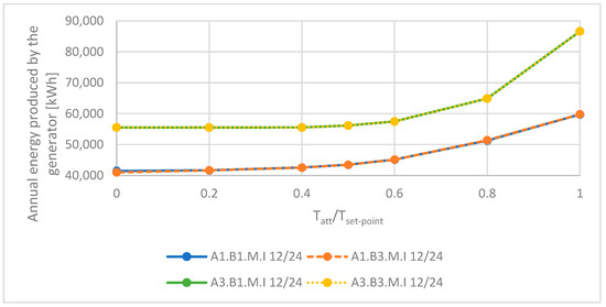
Figure 4.
Energy produced by the generator in operating mode with Tset-point for 12 h per day.
By analyzing the graph in Figure 5, it was possible to identify patterns similar to what was found regarding the characteristics of the curves for the four scenarios above; however, even on a visual level, it could be seen that the asymptotic value of the minimum energy generated was very similar for all the models. Due to these particular trends, the difference in the QH,gen,out,max/QH,gen,out,min ratio for light and heavy buildings was even more marked (3.19 and 2.31). Finally, if the maximum consumption was the same regardless of the hourly set-point combination, in the cases involving 4 h of set-point heating, the minimum energy consumption was significantly lower (differences ranging from approximately 16,000 kWh to approximately 28,000 kWh).
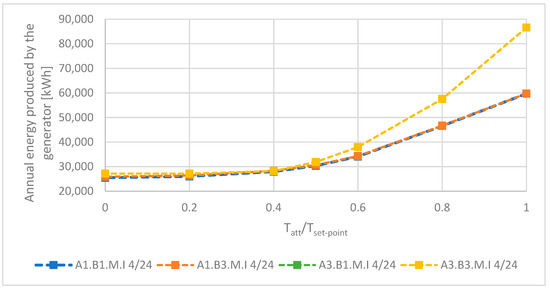
Figure 5.
Energy produced by the generator in operating mode with Tset-point for 4 h per day.
To complete the analysis, it may be useful to provide an overview of the difference in annual energy produced by the generator in cases with different set-point time bands. As is natural, for the 4 h daily set-point temperature models, the energy expenditure was lower compared to the equivalent 12 h models, and the attenuation temperature had a greater decrease: the trend was more than evident in Figure 6, which shows the results obtained for the A1.B1.M.I model.
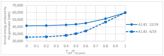
Figure 6.
Energy produced by the generator for the different daily set-point temperature durations in the A1.B1.M.I model.
The point of maximum deviation was found for a Tatt equal to 0 °C. It was precisely in this scenario that the experimental parameter γ was calculated, a mathematical function that made it possible to standardize the information provided by the graph for a subsequent comparison between all the models using the same homogeneous value. This procedure was carried out using the following formula:
where:
γ = ∆QH,gen,out,min/QH,gen,out,max
- ∆QH,gen,out,min is the difference between the QH,gen,out values at Tatt⁄Tset-point = 0 calculated in cases with Tset-point for 12 and 4 h daily;
- QH,gen,out,max is the value of QH,gen,out calculated when Tatt⁄Tset-point =1, i.e., when Tatt = Tset-point = 20 °C. Naturally, the value was the same for both 12 and 4 h daily at Tset-point.
This calculation, carried out for the single model, helped to quantify the impact that the width of the time band had on the energy expenditure of the building: if the value was close to zero, the generator produced the same amount of energy in the two scenarios, and therefore setting an hourly target of 12 h instead of 4 h made almost no difference. On the contrary, as γ increased, the “convenience” of the more restricted time slot increased, given that the thermal energy delta gradually increased.
Below is the comparison graph (Figure 7) between the values of γ obtained for each energy model studied.
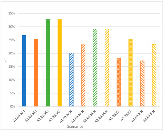
Figure 7.
Comparison of the γ value in all energy models.
From the histogram, it can be seen that the highest values detected for the experimental parameter γ were associated with models A3.B1.M.I and A3.B3.M.I, i.e., buildings with heavily insulated masonry and radiators with minimum potential that differed in terms of generator size. This meant that these models were more suitable for use with an hourly set-point adjustment over a 4 h period, since the annual energy savings were maximized. On the other hand, the building models that showed a smaller difference in thermal expenditure between the time slots were A1.B3.E.I and A1.B3.E.N, i.e., buildings with a huge generator and radiators and light masonry, insulated and non-insulated, respectively. This behavior, apparently, was in contrast to the assumption that a building with higher thermal inertia (A3) would have a similar energy expenditure for the two time slots analyzed, given that, once heated, the thermal inertia should decrease the energy consumption to maintain the set-point temperature. Conversely, a lighter building (A1) should be more “flexible”, i.e., heat up and cool down faster, widening the gap between the two cases. The results, however, showed diametrically opposite behavior. Initially, it was hypothesized that the cause of the lower γ for the light buildings was the higher denominator (QH,gen,out,max). However, by comparing the results shown in Figure 8, it is clear that this was not the case: the energy expenditure when the abscissa equals one, i.e., QH,gen,out,max, for model A3 (heavy) was certainly greater than the equivalent for A1, while the difference between the cases with 12 and 4 h set-point temperatures was evidently smaller for A1 with the abscissa equal to 0.
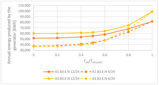
Figure 8.
Energy produced by the generator for the different set-point ranges in the models indicated in the legend.
In order to understand the causes of these results, we decided to consider a further comparison value that allowed us to evaluate the significance of the experimental parameter γ= (QH,gen,out,min ⁄ QH,gen,out,max)12, i.e., the ratio between the minimum energy and the maximum energy supplied in the 12 h per day set-point system. A comparison between the individual scenarios is shown via a histogram in Figure 9.
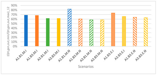
Figure 9.
Comparison of the (QH,gen,out,min ⁄ QH,gen,out,max)12 ratio for all energy models.
Furthermore, by combining the parameters γ and (QH,gen,out,min ⁄QH,gen,out,max)12 in a single graph, a dispersion of the values in the Cartesian plane was produced (Figure 10).
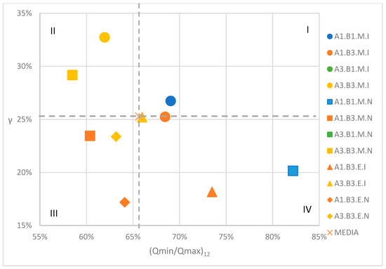
Figure 10.
Dispersion of the values in the γ–(QH,gen,out,min ⁄QH,gen,out,max)12 plane for all the energy models.
To increase the significance of this graph showing the dispersion of the points, it was decided to calculate the average value for all the scenarios, which was positioned in a barycentric manner, and from this to draw two orthogonal axes so as to be able to divide the cloud of points into four sectors. Considering that:
- A higher value of γ should indicate a building for which it is more energy-efficient to implement hourly set-point temperatures for 4 h per day;
- A low value of (QH,gen,out,min ⁄QH,gen,out,max)12 indicates an energy model for which the difference between operation with low attenuation temperatures and a regime with continuous operation involves a huge reduction in consumption;
It was natural to conclude that the models positioned in the second (II) quadrant, i.e., A3.B1.M.I, A3.B3.M.I, A3.B1.M.N, A3.B3.M.N, were those most compatible with time management at low attenuation temperatures and a few hours of set-point temperatures per day.
The first quadrant (I) represented the cases in which the difference in energy consumption between the 4 h and 12 h bands was high, but, at the same time, the minimum consumption for the 12 h regime was close to that under continuous operation. Since these situations are difficult to reconcile, this sector was almost empty, containing only the A1.B1.M.I model; however, it was actually positioned very close to the average of the different scenarios. In the third quadrant (III), significant energy savings were obtained by the implementation of an attenuation regime in comparison to the continuous case, while the choice of a shorter or longer time band was of little influence. The fourth and final sector (IV) contained the A1.B1.M.N and A1.B3.E.I models, for which there were few savings under an attenuation regime and a small difference between the time slot durations: these were therefore the cases in which the curve had the gentlest slope, i.e., the buildings for which continuous operation was advisable to avoid thermal discomfort, considering the similar consumption levels for the different scenarios.
It can also be noted that, generally, buildings with a small mass were farther to the right on the graph than their heavy counterparts: this meant that thermal inertia acted in favor of implementing an attenuation regime. This analysis offers interesting, but unclear, suggestions for the interpretation of the general picture, as it raises doubts about the consistency of the data obtained in relation to what was logically expected; all this leaves space for possible future developments in the study of this phenomenon.
A further element to underline in the operational differences between each model is represented by the operating hours of the generator. Figure 11 shows the number of operating hours month by month, under conditions of a Tset-point of 20 °C for 12 h a day and a Tatt equal to 10 °C, for models with minimum radiators and insulated masonry.
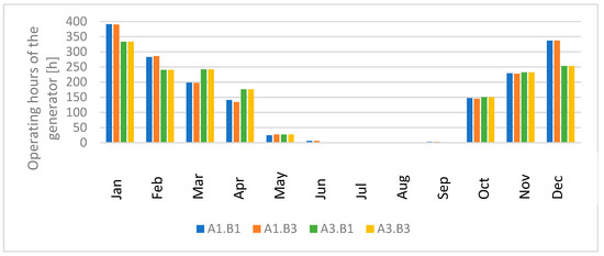
Figure 11.
Operating hours of the generator for models with 12 h per day of thermal set-point, Tatt = 10 °C, minimum radiators, and insulated masonry.
Naturally, the months in which the generator ran for the longest time were during winter, regardless of the simulation parameters. However, some peculiar differences can be noted: the generators in the models describing a building with a “light” mass ran for longer in winter than those in buildings with a “heavy” mass. The explanation for such a phenomenon could be found in the thermal inertia of buildings with a greater mass, which would counteract the dispersions. Similarly, in spring, the same inertia would put heavier buildings at a disadvantage; the mild climate certainly limits the impact of heat loss on energy requirements, thus highlighting the impact of the energy needed to heat the building: in fact, from the graph, it can be seen that in March, April, and October, the models with parameter A3 required the prolonged operation of the generator. Nonetheless, overall, a greater mass required less working time for the generator: 1650 h per year vs. 1750 h in the “light” case. This information could be made more complete by an analysis of the generator load factor. Figure 12 shows the distribution over the total operating hours of the generator operating mode for two models with different masses, taken from the four previously shown. It is evident that, even if it remained in operation for a greater number of hours, as deduced above, the generator of the model with a “light” mass operated for most of the time with a load factor lower than 25%, while the equivalent in a heavy-mass building had a higher average load factor.
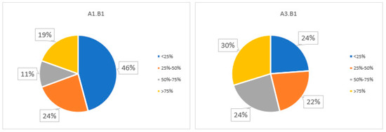
Figure 12.
Distribution of the load factor over the total operating hours for a model with a “light” mass (left) and for a model with a “heavy” mass (right).
We also compared the results obtained by modifying the Tatt within the same model, to maintain the same yardstick when evaluating the impact of this variable. We selected the A1.B1.M.I model, i.e., with a light mass, minimum generator and radiators, insulated masonry, and 12 h a day regime. Figure 13 shows the operating hours of the generator for each month calculated through the simulation.
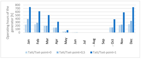
Figure 13.
Monthly hours of generator operation for the A1.B1.M.I model according to different Tatt values, set to 12 h a day of thermal set-point.
Naturally, the option that required the constant maintenance of 20 °C necessitated by far the longest operating time for the generator and, conversely, achieved a Tatt equal to 0 °C with the fewest operating hours; however, as can be seen from the graph in Figure 13, the number of operating hours for this latter model was more than comparable with the average case (for which Tatt was set at 10 °C): the difference was very large only in the months of January and December, and, overall, the difference between the two scenarios resulted in 315 more hours of operation per year. Given the greater expenditure, to evaluate whether maintaining a higher attenuation temperature was really useful for reaching the Tset-point, we decided to calculate the number of hours of discomfort in the two cases with Tatt = 0 °C and Tatt = 10 °C, i.e., the number of hours for which the building’s temperature was found to be below 20 °C in the designated 12 h time slot. Overall, the hours of discomfort for the model with a Tatt equal to 0 °C (249 h/year) were found to exceed by just one percentage point those of the model at 10 °C (219 h/year), if we relied on the total annual number of operating hours, despite the fact that the generator, in the second case, remained in operation for 23% (equal to 315 h) longer than if the attenuation temperature was lowered. At first glance, it would therefore seem more convenient to leave the Tatt equal to 0 °C, even if the final decision also depended on the importance attributed to the failure to reach the set-point temperature: it should in fact be emphasized that in the case of a Tatt equal 0 °C, on average, the discomfort level differed with respect to the Tset-point by over 2 °C, while in the other case, the difference was around 1.5 °C.
6. Discussion and Conclusions
This study concerned the impact of the system settings on the energy performance of a building. The energy analysis was carried out using simulation software by applying a dynamic hourly calculation regime on several models created by varying certain characteristic parameters related to the structure and the heating system.
The initial conditions for creating the energy models assumed two variable parameters, each defined by three distinct values, for an initial nine combinations. The two parameters chosen were:
- The thermal inertia of the building, represented by the recovery factors as a function of the mass of the building itself.
- The sizing of the heat generator according to the thermal power required by the building.
- The presence or absence of external insulation on the walls (I/N).
- The size of the radiators installed in the room in relation to the energy needs of the building.
By defining the empirical parameter γ as an index of the difference in energy consumption in relation to the time bands for regulating the thermal set-point, it was possible to catalog the behavior of the models, grouping them into four sectors. This study showed that for models with heavy masonry, the impact of the time band on the annual energy consumption was much lower than for models with light masonry. In addition, the operating hours and generator load factor results were examined for the different models. In buildings with a light mass, the generator ran for longer in winter than in those with a heavy mass, but the situation was reversed in spring. This behavior was probably due to the differences in thermal inertia, which, for models with heavy masonry, was advantageous in winter to counteract dispersions but unfavorable in spring, when thermal dispersions are more contained. However, a higher mass required less working time for the generator. Finally, we decided to compare the monthly operating hours within a single model, varying the attenuation temperatures, to evaluate whether maintaining a higher temperature outside the designated time slot was conducive to thermal comfort, despite the increased generator usage. The analysis showed that a lower attenuation temperature resulted in more hours of discomfort per year, but this disadvantage was negligible when compared with the additional operating hours required for a higher temperature.
Author Contributions
Conceptualization, S.Z.; data curation, S.Z.; methodology, S.Z. and L.E.Z.; validation, S.Z.; writing—original draft, I.F.; writing—review and editing, I.F., L.E.Z., S.Z. and B.M. All authors have read and agreed to the published version of the manuscript.
Funding
This research received no external funding.
Data Availability Statement
The authors confirm that the data supporting the findings of this study are available within the article.
Acknowledgments
The authors thank Alberto Mille for his contribution to the building modeling software and data analysis.
Conflicts of Interest
The authors declare no conflict of interest.
Appendix A
Below, we show the core equations used in the simulation software to calculate:
- Thermal energy;
- Analytical method for calculating generation losses.
Appendix A.1. Thermal Energy
The thermal energy required for winter air conditioning was divided into:
- Ideal requirement (QH,nd): the fundamental input data for calculating the primary energy requirements for heating. This requirement refers to the condition of uniform air temperature throughout the heated space and was calculated according to UNI/TS 11300-1 in continuous or intermittent operation depending on the intended use.
- Net ideal demand (QH’): from the useful thermal energy demand (QH,nd), any recovered losses (QW,lrh) from the DHW service were deducted, including a share of losses recovered from the final distribution across utilities, the recirculation network, the primary circuit, and the external accumulation tank in the DHW production plant. To calculate the net ideal requirement, the losses recovered from the domestic hot water production system were only those related to the duration of the heating activation period. If there were months with fewer days of activation than the duration of the month, the losses recovered were attributed proportionally to the number of days of activation.
- Actual requirement (Qhr): the net ideal requirement did not take into account the losses determined by the characteristics of the emission and regulation subsystems, foreseen or installed in the considered area. In fact, to calculate the effective requirement of the building (Qhr), i.e., the amount of thermal energy that had to be introduced into the rooms heated by the distribution network, negative factors were taken into account, such as:
- ○
- Greater losses towards the outside due to the non-uniform distribution of air temperature inside the heated environments (stratification) and losses towards the outside of the emission terminals due to conduction and/or radiation;
- ○
- Greater losses due to imperfect regulation and the possible non-utilization of free contributions included in the calculation of QH,nd, which translate into higher ambient temperatures rather than reductions in heat emission and positive factors, such as the transformation into heat of the electricity used in the terminal units.
The general expression for calculating the effective useful thermal energy (Qhr,i) that must be supplied to the i-th thermal zone is as follows:
where:
Qhr,i = QH,i’ + Ql,e,i + Ql,rg,i [kWh]
- Ql,e,i are the losses of the emission subsystem;
- Ql,rg,i are the losses of the control subsystem.
Appendix A.2. Analytical Method for Calculating Generation Losses
In addition to the performance values that must normally be supplied by the generator manufacturer, the analytical calculation method requires other values. These values are generally provided in the technical literature of the products; otherwise, it is necessary to use the default values.
The calculation method for these values was based on the following principles:
- The total operating time (tgn) of the generator (activation time) was divided into two parts:
- ○
- Operation with burner flame lit, ton;
- ○
- Waiting times with burner flame off (stand-by), toff.
The activation time is therefore expressed as: tgn = ton + toff.
- Losses were calculated separately for these two time periods.
During operation with the burner flame lit, the following losses were taken into account:
○ Sensible heat losses with burner on, Qch,on;
○ Generator casing losses, Qgn,env.
During the waiting times with the burner flame extinguished (stand-by), the following losses were taken into account:
○ Flue sensible heat loss with the burner off, Qch,off;
○ Generator casing losses, Qgn,env.
- Auxiliary energy was treated separately in relation to the appliances placed functionally before or after the combustion chamber:
- ○
- Qaux,af—auxiliary energy for appliances placed after the combustion chamber (primary circulation pumps operating for the entire activation period of the heat generator), tgn = ton + toff;
- ○
- Qaux,br—auxiliary energy for appliances upstream of the combustion chamber (in particular, the combustion air fan), operating only when the burner is on.
kaf and kbr are the recovered fractions of these auxiliary energies.
We therefore obtained:
- Qaux,af,rh = kaf × Qaux,af—thermal energy recovered by the appliances after the combustion chamber, operating for the entire period of the activation of the heat generator, tgn = ton + toff.
- Qaux,br,rh = kbr × Qaux,br—thermal energy recovered from appliances before the combustion chamber, operating only when the burner is on (i.e., only during ton).
The useful thermal energy supplied to the water leaving the generation subsystem is expressed as:
Qgn,out = Qgn,in + (Qaux,br,rh + Qaux,af,rh) − (Qch,on + Qch,off + Qgn,env) [Wh]
Appendix B
Below, supplementary input data used for the simulation are shown:
- Hourly climatic data referring to the chosen time period (Figure A1);
- Time profile assignment for the set-point temperatures within the thermal zone (Figure A2).
- Figure A1. Hourly climatic data referring to the chosen time period
- Figure A2. Time profile assignment for the set-point temperatures within the thermal zone

Figure A1.
Hourly climatic data referring to the chosen time period.
Figure A1.
Hourly climatic data referring to the chosen time period.


Figure A2.
Time profile assignment for the set-point temperatures within the thermal zone.
Figure A2.
Time profile assignment for the set-point temperatures within the thermal zone.

References
- Feng, C.; Meng, Q.; Zhang, Y. Theoretical and experimental analysis of the energy balance of extensive green roofs. Energy Build. 2010, 42, 959–965. [Google Scholar] [CrossRef]
- Pedrini, A.; Westphal, F.S.; Lamberts, R. A methodology for building energy modelling and calibration in warm climates. Build. Environ. 2002, 37, 903–912. [Google Scholar] [CrossRef]
- Erkoreka, A.; Garcia, E.; Martin, K.; Teres-Zubiaga, J.; Del Portillo, L. In-use office building energy characterization through basic monitoring and modelling. Energy Build. 2016, 119, 256–266. [Google Scholar] [CrossRef]
- Benitez, J.M.F.; del Portillo-Valde, L.A.; Pe, R. David Sosa Methodology to determine Energy Efficiency Strategies in Buildings sited in Tropical Climatic Zones. Case study, Buildings of the Tertiary Sector in the Dominican Republic. Energies 2022, 15, 4715. [Google Scholar] [CrossRef]
- Akhverdashvili, R.; Gulkanov, A.; Saiyan, S.; Modestov, K. Numerical Simulation of the Temperature Field of an Office Space with Three Types of Heating Systems; Notes in Civil Engineering book series (LNCE); Springer: Berlin, Germany, 2022; Volume 282. [Google Scholar]
- Crawley, D.B.; Hand, J.W.; Kummert, M.; Griffith, B.T. Contrasting the capabilities of building energy performance simulation programs. Build. Environ. 2008, 43, 661–673. [Google Scholar] [CrossRef]
- Attia, S.; Hensen, J.L.; Beltrán, L.; De Herde, A. Selection criteria for building performance simulation tools: Contrasting architects’ and engineers’ needs. J. Build. Perform. Simul. 2012, 5, 155–169. [Google Scholar] [CrossRef]
- Mahmud, K.; Amin, U.; Hossain, M.; Ravishankar, J. Computational tools for design, analysis, and management of residential energy systems. Appl. Energy 2018, 221, 535–556. [Google Scholar] [CrossRef]
- Clarke, J.; Hensen, J.; Hensen, J. Integrated building performance simulation: Progress, prospects and requirements. Build. Environ. 2015, 91, 294–306. [Google Scholar] [CrossRef]
- Haidong, W.; Zhiqiang, J.Z. Advances in building simulation and computational techniques: A review between 1987 and 2014. Energy Build. 2016, 128, 319–335. [Google Scholar] [CrossRef]
- Carlinia, M.; Castellucci, S.; Ceccarelli, I.; Rotondo, M.; Mennunia, A. Study of a thermal dispersion in buildings and advantages of ceramic coatings for the reduction of energy expenditure. Energy Rep. 2020, 6, 116–128. [Google Scholar] [CrossRef]
- Barone, G.; Buonomano, A.; Forzano, C.; Palombo, A. Building Energy Performance Analysis: An Experimental Validation of an In-House Dynamic Simulation Tool through a Real Test Room. Energies 2019, 12, 4107. [Google Scholar] [CrossRef]
- Attia, S.; Hamdy, M.; O’Brien, W.; Carlucci, S. Assessing gaps and needs for integrating building performance optimization tools in net zero energy buildings design. Energy Build. 2013, 60, 110–124. [Google Scholar] [CrossRef]
- Waltz, J.P. Computerized Building Energy Simulation Handbook; The Fairmont Press: Lilburn, GA, USA, 2000. [Google Scholar]
- Kenny, P.; Lewis, J.O. (Eds.) Tools and Techniques for the Design and Evaluation of Energy Efficient Buildings; European Commission DG XVII Thermie Action no. B 184; Energy Research Group, University College Dublin: Dublin, Ireland, 1995; Available online: https://www.upv.es/bin2/caches/miw/visfit?id=337092&idioma=C (accessed on 1 January 2023).


Disclaimer/Publisher’s Note: The statements, opinions and data contained in all publications are solely those of the individual author(s) and contributor(s) and not of MDPI and/or the editor(s). MDPI and/or the editor(s) disclaim responsibility for any injury to people or property resulting from any ideas, methods, instructions or products referred to in the content. |
© 2023 by the authors. Licensee MDPI, Basel, Switzerland. This article is an open access article distributed under the terms and conditions of the Creative Commons Attribution (CC BY) license (https://creativecommons.org/licenses/by/4.0/).