Role of Non-Adiabatic Capillary Tube in Water Cooler Performance

Abstract

In this paper, a numerical model of a capillary tube is developed. The considered expansion device is placed against the suction line at the inlet of the compressor. Wrapping the capillary tube around the suction line allows heat to be recovered by superheating the refrigerant leaving the evaporator. This increases the degree to which the fluid is superheated, preventing liquid droplets from entering the compressor and causing damage. The open-source software PYTHON is used for modelling the non adiabatic capillary tube, and the results are validated by comparing them with experimental tests. This study demonstrates that an accurate contact of the capillary tube with the suction line affects the superheating of the compressor inlet fluid by increasing its temperature by up to 5 degrees and produces an increase in COP of 3–4%. On the other hand, the length of the capillary tube affects the flow rate of the refrigerant circulating in the cycle; in particular, it is noted that a 300% increase in the capillary tube length leads to a decrease in the refrigerant flow rate of up to 50–60%.

1. Introduction

The past seven years have been the hottest ever recorded, according to all datasets compiled by the World Meteorological Organization [1]. As the planet warms, demand for cooling devices increases. Demand for space cooling has risen at an average pace of 4% per year since 2000. The number of units in operation has more than doubled since 2000, reaching over 2.2 billion units and accounting for 16% of the building sector’s final electricity consumption in 2021. According to the IEA report [2], the increased demand for cooling contributes to the increased emission of hydrofluorocarbons and CO₂ and thus has an impact on climate change. Worldwide, an estimated 3.6 billion cooling appliances are in use. The report says that if cooling is provided to everybody who needs it, this would require as many as 14 billion cooling appliances by 2050. A reduction in emissions could occur through a transition to more energy-efficient cooling. This would contribute substantially to the achievement of the Sustainable Development Goals. In this context, the importance of design technology to improve the energy efficiency of vapour compression cycles has been recognized. One of the main strands of research in recent years has been based on the study of the main components of reverse cycles to improve their performance: compressor, evaporator, condenser, and expansion device. The latter has been the subject of fewer studies than the other components. The capillary tube is an expansion device in a refrigeration system. It is the most suitable device for a system with less than 3 tons of refrigeration capacity, e.g., domestic refrigerators and window air-conditioners [3]. The advantages associated with using a capillary tube in place of a throttling valve are reliability due to the absence of moving parts, low cost, no maintenance, and reduced refrigerant charge. One of the parameters that most influences the operating conditions is the temperature of the environment in which the refrigeration machine works. For this reason, the capillary tube is used in applications for which the environment does not experience large temperature variations. The capillary tube can be adiabatic or diabatic [4]. In the adiabatic capillary tube, the refrigerant expands adiabatically. In a diabatic flow arrangement (Figure 1), the capillary tube is connected to the cold suction line of the compressor in a counterflow heat exchange arrangement. The advantage of using a diabatic capillary tube is a greater cooling effect and thus better system performance.

Although the CSLHX (Capillary–Suction Line Heat Exchanger) has extremely simple construction, the study and modelling of this component are far from trivial. Several complex phenomena can be encountered during operation: the simultaneous presence of liquid and vapour; phase change heat transfer; thermal contact between the two tubes not being guaranteed; and the achievement of sonic locking.

In recent years, the literature has been concerned with studying the influence of capillary tube use in vapour compression systems, but few studies have been conducted on the non-adiabatic helical configuration (Dubba and Kumar, 2017 [3]). Several studies can be found for non-adiabatic rectilinear configurations. K. C. Mendonca et al. 1998 [5] analysed the behaviour of two different capillary tube geometries with six different suction tube couplings. C. Melo et al. 2000 [6] studied the behaviour of R-134a fluid inside a straight, diabatic capillary tube concentric to the suction line, analysing how geometry and operating conditions affect the refrigerant flow rate. Ji Hwan Jeong et al. 2012 [7] developed a rectilinear capillary tube model in contact with the suction line to analyse the influence on COP and cooling capacity. In 2019, Rakesh Chechare et al. [8] were responsible for conducting a parametric analysis to study the effect of capillary tube diameter and degree of sub-cooling on performance parameters. They compared the lateral heat exchanger configuration with the concentric configuration and found that the lateral configuration gives better performance.

Regarding studies conducted on helical capillary tubes wrapped around the suction line, fewer contributions can be found in the literature. In 2009, Mohd. Kaleem Khan et al. [9] studied the influence of capillary tube geometrical parameters and degree of sub-cooling on refrigerant mass flow rate. Santhosh Kumar Dubba and Ravi Kumar [10] studied the behaviour of R600a through a helical capillary tube concentric to the suction line. From the study, results were extrapolated regarding the relationship between refrigerant mass flow rate and capillary tube geometry.

In the literature, a lack of works about helical capillary tubes wrapped externally around the compressor suction line can be noted, as well as a scarcity of data on the performance of ‘R600a’ and ‘R290’ fluids within these applications [3].

In this regard, the purpose of this work is to analyse the influence of the heat transfer area between the capillary tube and suction line on the cycle thermodynamic performance and on the refrigerant flow rate, in a configuration where the helical capillary tube is wrapped externally around the suction line. The analyses are conducted by varying the lateral exchange area and the length of the tube. Furthermore, the reported data will contribute to increase knowledge of R290 and R600a, which represent only 9 and 13% of the refrigerants considered in scientific research [3], respectively, supporting possible future applications of such natural refrigerants.

2. Materials and Methods

In order to evaluate the performance of the water cooler machine under different working conditions of the diabatic capillary tube, a mathematical model is implemented in PYTHON. The capillary tube model works by dividing the capillary tube into segments, and analysing piece by piece what happens to the working fluid by solving energy and mass balance equations. Although the ultimate goal is to obtain a model that can be used for different types of refrigeration machines, the focus is on commercially available water cooling machines, for domestic or office use, given their increasing relevance in the refrigeration sector.

The goal of the modelling is to obtain a tool to define the architecture of the capillary tube, and thus find the cycle operating temperatures, as well as how best to design the capillary tube in terms of geometry, i.e., tube length and diameter and refrigerant flow rate. For this reason, the independent variables within the model are the capillary tube length and the refrigerant flow rate. To achieve this, the model starts from the condensing pressure and proceeds by iterating the energy balance equations until the pressure reaches the evaporating pressure. In this way, the model can be used as a decision-making tool to achieve the working conditions established through the use of the capillary tube as an expansion device.

2.1. Solving Algorithm

As input, the program needs the type of refrigerant, condensation, evaporation temperatures, and the degree of subcooling, along with the geometric data of the capillary and suction tube. The cycle in Figure 2 is iterative, and proceeds by fixed pressure drop intervals $\Delta p$. The exit conditions are the achievement of evaporation pressure and sonic conditions. The outputs are the refrigerant flow rate or the length of the capillary tube, the vapour quality, and the enthalpy of the refrigerant entering the evaporator.

The code offers the option of being used from the refrigerant flow rate or the capillary tube length; depending on the usage, the capillary length and refrigerant flow rate, respectively, will be returned.

The capillary tube model is then fed into a simulation program of the entire thermodynamic cycle, Figure 3. As an input of the thermodynamic cycle, the output data of the capillary tube model are entered, i.e., the mass of refrigerant, the enthalpy of the fluid exiting the capillary, and, from the suction line temperature, the enthalpy of the fluid exiting the evaporator. As for the compressor, considering commercially available machines, the isentropic efficiencies of the compressors are extrapolated from manufacturers’ datasheets.

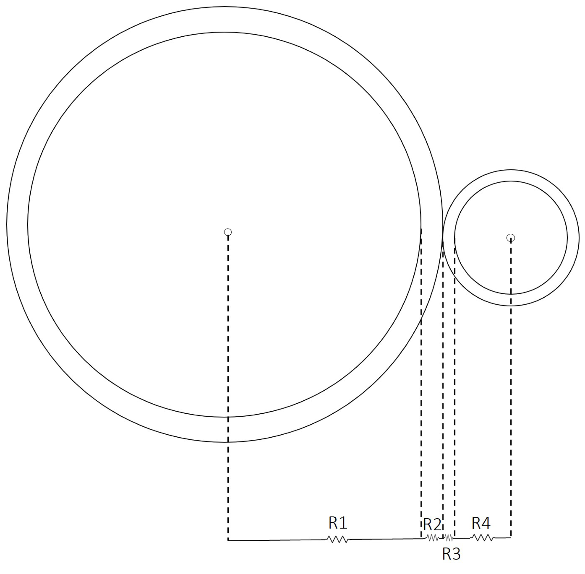
2.2. Mathematical Model

The non-adiabatic capillary tube has an initial adiabatic region where there is no contact between the capillary tube and the suction tube and a portion of the pipe wrapped around the suction tube. Furthermore, within each region, one can be found in both single-phase and two-phase flow conditions. Four cases can occur:

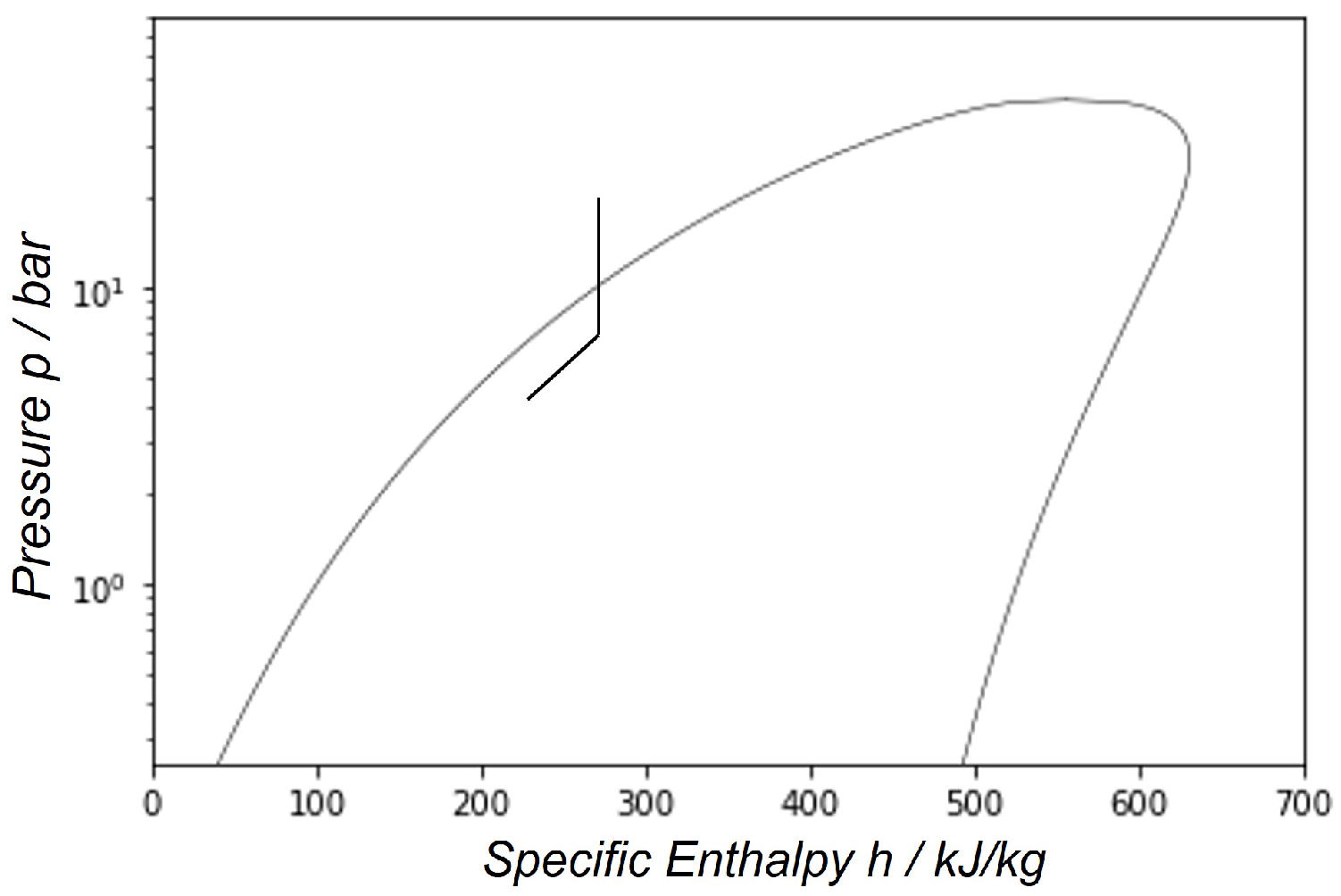
• The length of an adiabatic segment is less than the length of the single-phase part, while the non-adiabatic segment is entirely in the two-phase flow condition. Figure 4.
• The length of the adiabatic segment is greater than the length of the single-phase part, while the non-adiabatic segment is in the two-phase flow condition. Figure 5.
• The length of the adiabatic segment is less than the length of the single-phase part, and the fluid in the non-adiabatic segment after travelling a certain length of capillary returns to the subcooled fluid condition. Figure 6.
• The length of the adiabatic segment is greater than the length of the single-phase part, and the fluid in the non-adiabatic segment after travelling a certain length of capillary returns to the subcooled liquid condition. Figure 7.

In order to simplify the actual flow conditions without losing the main physical features, the following assumptions were made:

• Constant inner diameter and roughness of piping;
• Constant helix diameter of the capillary tube;
• Insensitivity to the helix diameter of the capillary tube; therefore, the model is not sensitive to the influence of the number of windings at the same capillary tube length;
• Capillary tube is helical throughout its length;
• Incompressible flow in single-phase regions;
• One-dimensional steady-state flow;
• Homogeneous two-phase flow;
• Negligible heat exchange with ambient air in the adiabatic capillary tube section;
• Thermodynamic equilibrium in which metastable flow phenomena are neglected.

The capillary tube can then be divided into two main sections: the adiabatic section, and the diabatic section, from which the following relationship is derived:

$$L_{tot}=L_{adiab}+L_{diaba}$$

(1)

In turn, each portion of the pipe has to be analysed according to the flow state:

$$L_{adiab}=L_{spad}+L_{tpad}$$

(2)

$$L_{diab}=L_{spd}+L_{tpd}$$

(3)

where $L_{spad}$, $L_{tpad}$, $L_{spd}$, and $L_{tpd}$ are the portion of the pipe in the single-phase adiabatic, two-phase adiabatic, single-phase diabatic, and two-phase diabatic sections, respectively.

The momentum balance under steady-state conditions is expressed as:

$$\frac{p_i}{{\rho }_{i}g}+\frac{V_i^2}{{\rho }_{i}g}+z_i=\frac{p_{i+1}}{{\rho }_{i+1}g}+\frac{V_{i+1}^2}{{\rho }_{i+1}g}+z_{i+1}+H_{loss}$$

(4)

where $H_{loss}$ is formed by a term representing the pressure losses due to the change in the cross-section at the capillary inlet (5), and a term representing the pressure losses due to friction with the walls of the tube (6):

$$\Delta p=k\frac{V^2}{2g}$$

(5)

$$\Delta p=f_{sp}\frac{L_{sp}}{D_{cap}}\frac{V^2}{2g}$$

(6)

The following equations for the friction factor $f_{sp}$, which are variations of the Mori and Nakayama [11] equation with varying coefficients taking the roughness of the tube wall into account, were formulated by Zhou and Zhang [12]:

$$f_{sp}=\frac{C_1{\left(\frac{D_{cap}}{D_e}\right)}^{0.5}}{{\left[Re{\left(\frac{D_{cap}}{D_e}\right)}^{2.5}\right]}^{1/6}}\left[1+\frac{C_2}{{\left[Re{\left(\frac{D_{cap}}{D_e}\right)}^{2.5}\right]}^{1/6}}\right]$$

(7)

$$C_1=1.88411177·{10}^{-1}+85.2472168\frac{ϵ}{D_{cap}}-4.63030629·{10}^4{\left(\frac{ϵ}{D_{cap}}\right)}^2+1.31570014·{10}^7{\left(\frac{ϵ}{D_{cap}}\right)}^3$$

(8)

$$C_2=6.79778633·{10}^{-2}+25.3880380\frac{ϵ}{D_{cap}}-1.06133140·{10}^4{\left(\frac{ϵ}{D_{cap}}\right)}^2+2.54555343·{10}^6{\left(\frac{ϵ}{D_{cap}}\right)}^3$$

(9)

By neglecting elevation changes from Equation (4), the length of the single adiabatic phase can be derived as (Bansal and Rupasinghe, 1998 [13]; Melo, 1992 [14]):

$$L_{sp}=\frac{D_{cap}}{f_{sp}}\left[\frac{2}{\rho V^2}\left(p_1-p_2\right)-k\right]$$

(10)

Taking into account the simplifications made and thus simplifying the mass terms and the changes in altitude, the energy balance in the two-phase flow region can be written as:

$$\frac{V_i^2}{2}+h_i=\frac{V_{i+1}^2}{2}+h_{i+1}+\left|q_{i+1}\right|$$

(11)

The continuity equation can be written as:

$$\dot{m}=\pi {\left(\frac{D_{cap}}{2}\right)}^2·V_i·{\rho }_i=\pi {\left(\frac{D_{cap}}{2}\right)}^2·V_{i+1}·{\rho }_{i+1}$$

(12)

Introducing the volumetric flow rate $\dot{G}$, the fluid velocity in the capillary can be defined as:

$$V_i=\frac{\dot{G}}{{\rho }_i}$$

(13)

$$V_{i+1}=\frac{\dot{G}}{{\rho }_{i+1}}$$

(14)

The heat exchanged between the capillary tube and suction line is evaluated using the correlations:

$$h_{i+1}=h_{fp,i+1}+x_{i+1}·{(h_g-h_f)}_{p,i+1}$$

(15)

$$v_{i+1}=v_{fp,i+1}+x_{i+1}·{(v_g-v_f)}_{p,i+1}$$

(16)

Thus, by making the appropriate substitutions, the vapour quality at point i+1 can be derived from Equation (11). The length of the section in the region of two-phase flow can be derived from the momentum balance equation:

$$mdV=\left(p\frac{\pi D^2{}_{cap}}{4}\right)-(p+dp)\frac{\pi D^2{}_{cap}}{4}-{\tau }_w{D}_{cap}\pi d{L}_{tp}$$

(17)

where ${\tau }_w$ is the tension, defined as:

$${\tau }_w=f_{tp}\frac{\rho V^2}{8}$$

(18)

The friction factor f for the two-phase flow region (Equation (19)) and helical tube is calculated with the following equation (Lin et al., 1991 [15]) from S. W. Churchill, 1977 [16]:

$$f_{tp}={\mathrm{\Phi }}^2{f}_{sp}\left(\frac{V_f}{V_{tp}}\right)$$

(19)

Then, from S. W. Churchill, 1977 [16]:

$${\mathrm{\Phi }}^2={\left[\frac{A_{sp}+B_{sp}}{A_{tp}+B_{tp}}\right]}^{1/8}\left[1+x\left(\frac{{\rho }_f}{{\rho }_g}-1\right)\right]$$

(20)

$$A_{sp}={\left[2457ln\left(\frac{1}{{\left(\frac{7}{R{e}_{sp}}\right)}^{0.9}+0.27\left(\frac{ϵ}{D_{cap}}\right)}\right)\right]}^{16}$$

(21)

$$A_{tp}={\left[2457ln\left(\frac{1}{{\left(\frac{7}{R{e}_{tp}}\right)}^{0.9}+0.27\left(\frac{ϵ}{D_{cap}}\right)}\right)\right]}^{16}$$

(22)

$$B_{sp}={\left(\frac{37530}{R{e}_{sp}}\right)}^{16}$$

(23)

$$B_{tp}={\left(\frac{37530}{R{e}_{tp}}\right)}^{16}$$

(24)

$$R{e}_{sp}=\frac{\dot{G}{D}_{cap}}{{\mu }_{sp}}$$

(25)

$$R{e}_{tp}=\frac{\dot{G}{D}_{cap}}{{\mu }_{tp}}$$

(26)

The heat flux $|q_{i+1}|$ transferred from the fluid in the capillary tube to the fluid in the suction line is evaluated as:

$$|Q_{i+1}|=U·A_{ex}·(T_i-T_j)$$

(27)

$$|q_{i+1}|=\frac{|Q_{i+1}|}{\dot{m}}$$

(28)

The contact area between the capillary tube and the suction line was evaluated as a portion of the outer area of the capillary, so later assessments were made regarding the influence of more or less precise winding on cycle performance.

$$A_{sc}=d{L}_{tp}·D_{cap}·\pi ·f$$

(29)

The resistive method Figure 8 is used to determine the overall heat transfer coefficient U:

$$\frac{1}{U{A}_{ex}}=R_1+R_2+R_3+R_4=\frac{1}{{\alpha }_{sl}{A}_{sl}}+\frac{ln\left(\frac{D_{sl,ex}}{D_{sl,in}}\right)}{2\pi k_{wsl}{L}_{sl}}+\frac{ln\left(\frac{D_{ct,ex}}{D_{ct,ex}}\right)}{2\pi k_{wct}{L}_{ct}}+\frac{1}{{\alpha }_{ct}{A}_{ct}}$$

(30)

where $k_w$, ${\alpha }_{sl}$, and ${\alpha }_{ct}$ are the tube perimeter conductivity and convective heat transfer coefficients of the suction tube and the capillary tube, respectively. Analysing the order of magnitude of the heat transfer coefficients showed that the convective heat transfer coefficient on the capillary tube side is three orders of magnitude greater than the heat transfer coefficient on the suction line side. Thus, the resistance R4 can be neglected, along with the conductive resistance of the walls of the two tubes, R2 and R3. Thus, the overall heat transfer coefficient can be calculated as follows, from the Gnielinski correlation [17]:

$$U={\alpha }_{sl}=Nu=\frac{\left(\frac{f_{ref}}{8}\right)(R{e}_{ref}-1000)P_{ref}}{1+12.7\sqrt{\frac{f_{ref}}{8}}(P{r}_{ref}^{2/3}-1)}·\frac{\lambda }{D_{sl,in}}$$

(31)

$$P{r}_{ref}=\frac{\mu c_p}{\lambda }$$

(32)

where $\mu$ is the dynamic viscosity and $f_{ref}$ is the friction factor within the suction line, evaluated using the Darcy–Weisbach correlation from Kamel Sigar Hmood et al. [18]:

$$f_{ref}=\frac{1}{{(0.79lnR{e}_{ref}-1.64)}^2}$$

(33)

The heat absorbed by the vapour from the suction line is considered to be the same as that given by the refrigerant on the capillary side. Therefore, we find:

$$|q_{i+1}|=h_{8i}-h_8$$

(34)

where $h_8$ is the initial enthalpy of the refrigerant in the suction line and $h_{8i}$ is the enthalpy of the refrigerant after heat exchange.

2.3. Literature and Experimental Validation

The capillary tube model is validated with data from two types of refrigerants, R134a and R600a, from Bansal and Wang [19]. The vapour quality at the capillary tube outlet and the refrigerant flow rate are the parameters used for the comparison. Given the same length and inner diameter of the capillary tube, the condensing temperature, the evaporation temperature, and the type of refrigerant, the comparison yielded the following results:

• The comparison with data obtained with R134a shows a deviation of 0–10% for vapour quality and a deviation that stabilizes around 16–17% for refrigerant flow rate.
• The comparison with data obtained with R600a shows a deviation of 2–5% for vapour quality and of 11–13% for refrigerant flow rate.

The non-adiabatic capillary tube model is also validated using three water-cooling machines. Each machine has its cooling capacity and its coupling configuration between the capillary tube and compressor suction line. The model as designed allows for adaptation to all configurations.

From the experimental measurements, performed on real machines for water cooling, are extrapolated data on evaporation temperature, condensation temperature, and the temperature of water in the tank over a certain time interval. Starting from these values, the actual heat output data, necessary to make the tank temperature drop by the measured quantity, were compared with the data extrapolated from the model. The comparison showed that the error between the extrapolated and measured data is between 4% and 15%.

3. Results

In order to evaluate and quantify the influence of the coupling between the capillary tube and suction line, sensitivity analyses are conducted.

As revealed in the review work conducted by Dubba and Kumar [3], from 2006 to 2016 only a small percentage of work on capillary tubes in the literature used propane “R290” and isobutane “R600a” as refrigerants, at 9% and 13% of the works found, respectively. Therefore, analyses using propane and isobutane are conducted in this research work, the results of which are given below.

First, sensitivity analysis is conducted on the lateral exchange area. By establishing as the maximum exchange area the half outer circumference of the capillary tube multiplied by the length of the capillary tube, f is a multiplicative coefficient indicating a fraction of the maximum area.

Table 1. Sensitivity analysis with respect to lateral heat transfer area. $T_{cond}$ = 54 °C, $T_{evap}$ = −3.7 °C, $\Delta$$T_{sub}$ = 3 °C, $L_{ct}$ = 2.2 m, $D_{ct}$ = 0.9 mm, refrigerant = R290.

f	Tsl (K)	%	COP	%	Qf (W)	%	m (kg/h)	%	x	%
0.1	279.82	0.0	1.937	0.0	372.29	0.0	5.262	0.0	0.3764	0.0
0.2	280.19	0.1	1.943	0.3	374.94	0.7	5.273	0.2	0.3748	0.4
0.3	280.57	0.3	1.949	0.6	377.59	1.4	5.285	0.4	0.3732	0.9
0.4	280.94	0.4	1.954	0.9	380.27	2.1	5.296	0.7	0.3716	1.3
0.5	281.31	0.5	1.960	1.2	382.94	2.9	5.308	0.9	0.3700	1.7
0.6	281.68	0.7	1.966	1.5	385.63	3.6	5.320	1.1	0.3684	2.1
0.7	282.05	0.8	1.971	1.8	388.34	4.3	5.331	1.3	0.3668	2.6
0.8	282.42	0.9	1.977	2.1	391.07	5.0	5.343	1.5	0.3652	3.0
0.9	282.79	1.1	1.983	2.3	393.79	5.8	5.355	1.8	0.3636	3.4
1.0	283.16	1.2	1.988	2.6	396.55	6.5	5.368	2.0	0.3620	3.8

and

Table 2. Sensitivity analysis with respect to lateral heat transfer area. $T_{cond}$ = 54 °C, $T_{evap}$ = −3.7 °C, $\Delta$$T_{sub}$ = 3 °C, $L_{ct}$ = 2.2 m, $D_{ct}$ = 0.66 mm, refrigerant: R600a.

f	Tsl (K)	%	COP	%	Qf (W)	%	m (kg/h)	%	x	%
0.1	279.86	0.0	2.056	0.0	70.54	0.0	1.024	0.0	0.3571	0.0
0.2	280.28	0.2	2.066	0.5	71.46	1.3	1.027	0.3	0.3554	0.5
0.3	280.69	0.3	2.075	1.0	72.26	2.4	1.031	0.6	0.3537	1.0
0.4	281.10	0.4	2.085	1.5	73.16	3.7	1.034	1.0	0.3520	1.4
0.5	281.52	0.6	2.095	2.0	74.08	5.0	1.038	1.3	0.3503	1.9
0.6	281.93	0.7	2.105	2.4	75.01	6.3	1.041	1.7	0.3486	2.4
0.7	282.34	0.9	2.112	2.8	75.65	7.2	1.045	2.0	0.3469	2.9
0.8	282.75	1.0	2.122	3.2	76.55	8.5	1.048	2.4	0.3452	3.3
0.9	283.16	1.2	2.131	3.7	77.47	9.8	1.052	2.7	0.3435	3.8
1.0	283.57	1.3	2.140	4.1	78.41	11.2	1.056	3.1	0.3418	4.3

show the values of suction line temperature, COP, cooling capacity, refrigerant flow rate, and vapour quality as the f-factor varies, with the use of R290 and R600a, respectively. Next to each value is also shown the relative variation with respect to the first iteration data. The data are extrapolated by fixing the condensation and evaporation temperatures, the capillary tube length and diameter, and the superheating degree.

The results show that more accurate contact results in an increase in the degree of superheating of the compressor inlet fluid, and an increase of up to 3% in COP and refrigerant flow rate. The use of one fluid versus another does not affect the trend in COP or compressor inlet temperature, but does affect the heat capacity, which is a property of the fluid itself.

Next, the influence of capillary tube length on machine performance is analysed. Based on the assumptions made about the helix diameter, the increase or decrease in the length of the capillary tube corresponds to an increase or decrease in its windings around the suction tube.

Table 3. Sensitivity analysis with respect to capillary tube length. $T_{cond}$ = 54 ${}^{\circ }$C; $T_{evap}$ = −3.7 ${}^{\circ }$C; $\Delta$$T_{sub}$ = 3 ${}^{\circ }$C; $D_{ct}$ = 0.9 mm; f = 1; refrigerant: R290.

L (m)	Tsl (K)	%	COP	%	Qf (W)	%	m (kg/h)	%	x	%
1.0	281.34	0.0	2.018	0.0	703.04	0	9.463	0	0.3498	0.0
1.1	281.54	0.1	2.010	−0.4	655.35	−7	8.841	−7	0.3546	0.8
1.2	281.75	0.1	2.005	−0.7	615.99	−12	8.330	−12	0.3548	1.4
1.3	281.95	0.2	2.001	−0.9	582.85	−17	7.889	−17	0.3564	1.9
1.4	282.16	0.3	1.998	−1.0	554.43	−21	7.507	−21	0.3577	2.3
1.5	282.37	0.4	1.996	−1.1	529.82	−25	7.173	−24	0.3585	2.5
1.6	282.59	0.4	1.995	−1.2	508.29	−28	6.878	−27	0.3592	2.7
1.7	282.80	0.5	1.994	−1.2	489.17	−30	6.614	−30	0.3596	2.8
1.8	283.22	0.7	2.001	−0.9	468.37	−33	6.298	−33	0.3577	2.3
1.9	283.51	0.8	2.002	−0.8	449.84	−36	6.038	−36	0.3576	2.3
2.0	283.80	0.9	2.003	−0.8	433.43	−38	5.805	−39	0.3574	2.2
2.1	284.10	1.0	2.005	−0.7	418.87	−40	5.596	−41	0.3571	2.1
2.2	284.40	1.1	2.007	−0.6	405.79	−42	5.407	−43	0.3566	2.0
2.3	284.70	1.2	2.009	−0.4	394.01	−44	5.236	−45	0.3560	1.8
2.4	285.00	1.3	2.012	−0.3	383.31	−45	5.079	−46	0.3553	1.6
2.5	285.30	1.4	2.015	−0.2	373.57	−47	4.936	−48	0.3546	1.4
2.6	285.61	1.5	2.018	0.0	364.68	−48	4.803	−49	0.3538	1.1
2.7	285.91	1.6	2.022	0.2	356.48	−49	4.680	−51	0.3529	0.9
2.8	286.22	1.7	2.025	0.3	348.94	−50	4.567	−52	0.3520	0.6
2.9	286.53	1.8	2.029	0.5	341.96	−51	4.460	−53	0.3510	0.4
3.0	286.84	2.0	2.032	0.7	335.50	−52	4.362	−54	0.3500	0.1

,with R290 as the refrigerant fluid and with a capillary tube diameter of 0.9 mm, and

Table 4. Sensitivity analysis with respect to capillary tube length $T_{cond}$ = 54 ${}^{\circ }$C; $T_{evap}$ = −3.7 ${}^{\circ }$C; $\Delta$$T_{sub}$ = 3 ${}^{\circ }$C; $D_{ct}$ = 0.66 mm; f = 1; refrigerant: R600a.

L (m)	Tsl (K)	%	COP	%	Qf (W)	%	m (kg/h)	%	x	%
1.0	279.45	0.0	2.133	0.0	172.32	0	2.422	0	0.3294	0.0
1.1	281.48	0.7	2.134	0.1	135.31	−21	1.877	−22	0.3329	1.1
1.2	281.79	0.8	2.128	−0.2	124.39	−28	1.727	−29	0.3354	1.8
1.3	282.09	0.9	2.126	−0.3	115.79	−33	1.608	−34	0.3369	2.3
1.4	282.39	1.1	2.125	−0.4	108.71	−37	1.509	−38	0.3379	2.6
1.5	282.70	1.2	2.125	−0.4	102.86	−40	1.425	−41	0.3385	2.8
1.6	283.02	1.3	2.123	−0.4	97.54	−43	1.353	−44	0.3387	2.8
1.7	283.33	1.4	2.125	−0.4	93.25	−46	1.290	−47	0.3386	2.8
1.8	283.65	1.5	2.127	−0.3	89.51	−48	1.235	−49	0.3384	2.7
1.9	283.96	1.6	2.130	−0.1	86.22	−50	1.186	−51	0.3380	2.6
2.0	284.28	1.7	2.133	0.0	83.33	−52	1.143	−53	0.3375	2.4
2.1	284.60	1.8	2.137	0.2	80.72	−53	1.104	−54	0.3368	2.3
2.2	284.92	2.0	2.140	0.4	78.41	−54	1.069	−56	0.3361	2.0
2.3	285.24	1.1	2.140	0.3	75.84	−56	1.036	−57	0.3353	1.8
2.4	285.56	2.2	2.144	0.5	73.92	−57	1.007	−58	0.3344	1.5
2.5	285.88	2.3	2.148	0.7	72.16	−58	0.980	−60	0.3335	1.3
2.6	286.20	2.4	2.152	0.9	70.57	−59	0.955	−61	0.3326	1.0
2.7	286.53	2.5	2.156	1.1	69.10	−60	0.932	−62	0.3315	0.7
2.8	286.85	2.7	2.160	1.3	67.73	−61	0.910	−62	0.3305	0.3
2.9	287.17	2.8	2.165	1.5	66.47	−61	0.890	−63	0.3294	0.0
3.0	287.49	2.9	2.170	1.8	65.32	−62	0.871	−64	0.3283	−0.3

, with R600a as the refrigerant fluid and with a capillary tube diameter of 0.66 mm, show the values of suction line temperature, COP, cooling capacity, refrigerant flow rate, and vapour quality as the length of the capillary tube changes. A factor of $f=1$ is used to define the exchange area. As for the analyses shown in Table 1 and Table 2, the data are extrapolated by fixing the condensation and evaporation temperatures, the capillary tube length and diameter, and the superheating degree.

The tables show that an increase in capillary tube length results in an increase in compressor inlet fluid temperature, and a decrease in refrigerant flow rate of up to 50%, leading to a decrease in refrigeration capacity. The COP, on the other hand, does not undergo changes that can be considered significant when varying the length of the capillary tube and keeping the operating conditions intact.

4. Conclusions

This paper presents the effects of capillary tube length and the heat exchange area of the suction line on the performance of a commercial water cooler machine, in order to define the architecture of the capillary tube, in terms of geometry, i.e., tube length and diameter, and refrigerant flow rate, knowing the operating temperatures of the cycle, and the required performance.

The conclusions that can be drawn from this study are as follows:

• An increase in the f-factor, leading to a more accurate coupling between the capillary tube and suction line, brings as an advantage an increase in the degree of superheating of the refrigerant entering the compressor, reducing the risk due to the presence of liquid in the compressor. On the other hand, the COP increase is almost negligible, in the order of 3%, in line with data in the literature (Ji Hwan Jeong, 2012 [7]).
• The increase in the capillary tube length of 300% has an influence on the degree of overheating and on the decrease in refrigerant charge of up to 60%, which contributes to charge reduction but, in turn, causes a decrease in cooling capacity.

References

- World Meteorogical Organization. Available online: https://public.wmo.int/en/media/press-release/2021-one-of-seven-warmest-years-record-wmo-consolidated-data-shows (accessed on 30 November 2022).
- IEA. Cooling Emissions and Policy Synthesis Report. Paris. License: CC BY 4.0. 2020. Available online: https://www.iea.org/reports/cooling-emissions-and-policy-synthesis-report (accessed on 30 November 2022).
- Dubba, S.K.; Kumar, R. Flow of refrigerants through capillary tubes: A state-of-the-art. Exp. Therm. Fluid Sci. 2017, 81, 370–381. [Google Scholar] [CrossRef]
- Khan, M.K.; Kumar, R.; Sahoo, P.K. Flow characteristics of refrigerants flowing through capillary tubes—A review. Appl. Therm. Eng. 2009, 29, 1426–1439. [Google Scholar] [CrossRef]
- Mendonca, K.C.; Melo, C.; Ferreira, R.T.S.; Pereira, R.H. Experimental Study on Lateral Capillary Tube-Suction Line Heat Exchangers. In Proceedings of the International Refrigeration and Air Conditioning Conference, West Lafayette, IN, USA, 14–17 July 1998; p. 450. Available online: http://docs.lib.purdue.edu/iracc/450 (accessed on 12 January 2023).
- Melo, C.; Zangari, J.M.; Ferreira, R.T.S.; Pereira, R.H. Experimental Studies on Non-Adiabatic Flow of HFC-134a Through Capillary Tubes. In Proceedings of the International Refrigeration and Air Conditioning Conference, West Lafayette, IN, USA, 25–28 July 2000; p. 496. Available online: http://docs.lib.purdue.edu/iracc/496 (accessed on 12 January 2023).
- Jeong, J.H.; Park, S.-G.; Sarker, D.; Chang, K.S. Numerical simulation of the effects of a suction line heat exchanger on vapor compression refrigeration cycle performance. J. Mech. Sci. Technol. 2012, 26, 1213–1226. [Google Scholar] [CrossRef]
- Chechare, R.; Ramaswamy, S.; Mahapatra, A. Numerical simulation of refrigerant flow and heat tranfer in a non-adiabatic capillary tube in refrigerator. Int. J. Mech. Prod. Eng. 2019, 7, 82–86. [Google Scholar]
- Khan, M.K.; Kumar, R.; Sahoo, P.K. Experimental investigation on diabatic flow of R-134a through spiral capillary tube. Int. J. Refrig. 2009, 32, 261–271. [Google Scholar] [CrossRef]
- Dubba, S.K.; Kumar, R. Experimental investigation on flow of R-600a inside a diabatic helically coiled capillary tube: Concentric configuration. Int. J. Refrig. 2018, 86, 186–195. [Google Scholar] [CrossRef]
- Mori, Y.; Nakayama, W. Study on forced convective heat tranfer in curved pipes. Int. J. Heat Mass Transf. 1967, 10, 37–59. [Google Scholar] [CrossRef]
- Guobing, Z.; Yufeng, Z. Numerical and experimental investigations on the performance of coiled adiabatic capillary tubes. Appl. Therm. Eng. 2006, 26, 1106–1114. [Google Scholar]
- Bansal, P.K.; Rupasinghe, A.S. An homogeneous model for adiabatic capillary tubes. Appl. Therm. Eng. 1998, 18, 207–219. [Google Scholar] [CrossRef]
- Guobing, Z.; Yufeng, Z. Modelling Adiabatic Capillary Tubes: A Critical Analysis. In Proceedings of the International Refrigeration and Air Conditioning Conference, 1992; p. 147. Available online: http://docs.lib.purdue.edu/iracc/147 (accessed on 12 January 2023).
- Lin, S.; Kwok, C.C.K.; Li, R.-Y.; Chen, Z.-H.; Chen, Z.-Y. Local Frictional Pressure Drop During Vaporization of R-12 through Capillary Tubes. Int. J. Multiph. Flow 1991, 17, 95–102. [Google Scholar] [CrossRef]
- Churchill, S.W. Friction equation spans all fluid flow regimes. Int. J. Chem. Eng. 1977, 84, 91–92. [Google Scholar]
- Gneilinski, V. New equations for heat and mass transfer in turbulent pipe and channel flow. Int. J. Chem. Eng. 1976, 16, 359–368. [Google Scholar]
- Hmood, K.S.; Pop, H.; Apostol, V.; Qaisy, S.A.; Badescu, V. Steady-state performance of capillary tubes for small-scale vapour compression systems using different refrigerants. Int. J. Refrig. 2021, 130, 87–98. [Google Scholar] [CrossRef]
- Bansal, P.K.; Wang, G. Numerical analysis of choked refrigerant flow in adiabatic capillary tubes. Appl. Therm. Eng. 2004, 24, 851–863. [Google Scholar] [CrossRef]