Article

Electric Vehicle Fast Charging: A Congestion-Dependent Stochastic Model Predictive Control under Uncertain Reference

by
Alessandro Di Giorgio
1,2,*,
Emanuele De Santis
1,2,*,
Lucia Frettoni
1,
Stefano Felli
1 and
Francesco Liberati
1,2
1
Department of Computer, Control and Management Engineering “Antonio Ruberti” (DIAG), University of Rome “La Sapienza”, Via Ariosto, 25, 00185 Rome, Italy
2
Consortium for the Research in Automation and Telecommunications (CRAT), Via Giovanni Nicotera, 29, 00185 Rome, Italy
*
Authors to whom correspondence should be addressed.
Energies 2023, 16(3), 1348; https://doi.org/10.3390/en16031348
Submission received: 29 December 2022 / Revised: 19 January 2023 / Accepted: 24 January 2023 / Published: 27 January 2023

Abstract

:
This paper presents a control strategy aimed at efficiently operating a service area equipped with stations for plug-in electric vehicles’ fast charging, renewable energy sources, and an electric energy storage unit. The control requirements here considered are in line with the perspective of a service area operator, who aims at avoiding peaks in the power flow at the point of connection with the distribution grid, while providing the charging service in the minimum time. Key aspects of the work include the management of uncertainty in the charging power demand and generation, the design of congestion and state-dependent weights for the cost function, and the comparison of control performances in two different hardware configurations of the plant, namely BUS and UPS connection schemes. All of the above leads to the design of a stochastic model predictive controller aimed at tracking an uncertain power reference, under the effect of an uncertain disturbance affecting the output and the state of the plant in the BUS and UPS schemes respectively. Simulation results show the relevance of the proposed control strategy, according to an incremental validation plan focused on the tracking of selected references, the mitigation of congestion, the stability of storage operation over time, and the mitigation of the effect of uncertainty.

1. Introduction

The ongoing shift to electromobility will require significant investments to develop a pervasive recharging infrastructure, which is safely and efficiently integrated into the electrical energy system. In this paper, we focus on the control of a “service area” for Plug-in Electric Vehicles (PEVs), i.e., the e-mobility equivalent of traditional petrol stations, where several charging stations provide a fast charging service to the PEVs [1].
One of the key challenges faced by the Service Area Operator is given by the high power levels involved in the fast charging process, which are necessary for acceptable recharging times for the drivers. Even few fast charging sessions active at the same time can cause power flows at the Point of Connection (POC) of the service area with the grid of several tens or hundreds of kW, which implies for the Service Area Operator (and, in turn, for the drivers) high costs for the operation of the service area; these costs are high enough to potentially make the service area concept infeasible from the business point of view.
For this reason, several papers have proposed the introduction into the service area of a stationary Energy Storage System (ESS) (to alleviate the effort for the grid, by contributing through the ESS to the peak power requests from PEVs, thus reducing the power flow at the POC), and of renewable power generators (which can alleviate the power peaks at the POC by providing a source of clean energy for recharging the PEVs). Even if the ESS may alleviate the load at the POC, its intervention capabilities depend on its current state-of-charge and on its capacity, which has to be properly taken into account in the operation of the service area.
Another challenge associated with the operation of the service area is given by the uncertainty associated with the PEV power demand (which depends on the drivers’ arrival time, the user charging request, etc.), and with the renewable power production.
In light of the above, in this paper, a stochastic Model Predictive Control (MPC) algorithm is proposed for the control of a service area equipped with an ESS and with renewable energy generators. Motivated by the above business challenge, we take the perspective of the Service Area Operator, and assume as the main control goal that of reaching a cost-effective operation of the service area, which can be achieved by reducing the power flow at the POC (the main cost driver). The POC power flow reduction is achieved on one side by controlling the ESS (which is used to balance the ongoing charging sessions), and also by controlling the actual charging power provided to the PEVs (this second control action can help the Service Area Operator to avoid to oversize the ESS in order to face high-congestion periods in the service area). While ESS control does not directly affect the drivers’ charging experience, the control of PEV recharging power obviously does; therefore, it is essential that the proposed controller provides to all the PEVs as much as possible the exact amount of power that they request (typically, the maximum possible charging power, in order to minimize the recharging times).
In light of the above, the three fundamental control requirements considered in this study are:
  • The reduction of the power flow at the POC of the service area with the main grid, which is essential in order to reduce operation costs of the service area;
  • The tracking of the charging power demand for each charging PEV (i.e., the controller must strive to assign to each PEV the power it requires), which is needed in order to assure minimum charging times for the drivers;
  • A third requirement is related with the operation of the ESS. It is desirable to avoid the ESS to become fully depleted during operation, since in this case, it cannot contribute to balance future charging demand peaks.

1.1. Literature Review

A broad literature is dedicated to the service area control problem. The contributions mainly differ for the considered scenario, the involved requirements, and the control methodology employed. Among the continuous time control methodologies, calculations of variations and the Pontryagin Minimum Principle (PMP) have found numerous applications in hybrid vehicle control (see, e.g., [2,3,4]) and in microgrid control [5]. The natural discrete-time counterpart of PMP, i.e., MPC, has been widely applied as well (see, e.g., [6,7]).
The present paper extends the previous work [8], where a continuous time method for the optimal control of an ESS in a fast-charging service area is proposed, based on the PMP. In [8], two possible hardware configurations for the service area were presented, highlighting their advantages and disadvantages. The control method proposed in [8] is optimal in minimizing the power flow at the POC, while ensuring that all the drivers are served with no delays in the charging process. However, the method in [8] is based on the complex PMP theory, which provides a closed loop and closed-form solution for the controller only in simple settings (e.g., constraints on the state and the control are ignored in [8]). In this paper, the formulation proposed in [8] is extended, by also modeling the ESS power losses, and by including additional control flexibility, given by the possibility of controlling the power set point of the recharging sessions, to reduce it in times of significant congestion (to help alleviate the stress on the POC). The problem is solved via the MPC principle, which is effective in providing a solution in this complex case. A first deterministic formulation of the service area control problem with MPC has been recently proposed by the authors in [9], in which, however, the charging processes are assumed to happen uncontrolled, at the power requested by the driver (typically, at maximum power). In the present paper, instead, the formulation is extended to the stochastic MPC case (i.e., contrary to [9], we do not assume here a perfect knowledge of the future charging demand), and the flexibility of controlling the charging power provided by the charging sessions is also considered.
Some recent works specifically focused on the optimization of fast-charging operations in a service area.
In [10], Ding et al. studied the optimal sizing and management of an ESS installed in a charging area for electric buses. They show how the ESS can significantly reduce the peak power from the electric grid when several electric buses are charging at the same time. While [10] focused on ESS control, as a mean to optimize the operation of the service area, in the present paper, we also include the control of the power delivered to the charging PEVs, which can contribute to reducing the peak power at the point of connection with the grid during high congestion times.
In [11], Sun studied the optimal design for fast EV charging stations with wind, PV power, and ESS, and a power scheduling strategy to minimize costs and pollution. The proposed solution method is a heuristic one. In the present paper, we also address the minimization of the power flow at the POC, and we propose to use an exact solving method (MPC).
In [12], Leonori et al. designed an energy management system for a public fast-charging station in a grid-connected nanogrid. The proposed control strategy is based on a fuzzy logic controller. The use of a fuzzy logic based control is motivated by the authors by the stochastic nature of fast charging demand, which prompted the authors to exclude a priori MPC methods, which, in their deterministic formulation, are indeed highly dependent on prediction accuracy. In this paper, we address this issue by proposing a stochastic MPC formulation, which assumes the knowledge of the expected value of the power demanded by the PEVs, which is information available to the service area operators.
In [13], Kucevic et al. proposed a method for reducing the charging peak power in urban distribution grids with a high share of PEVs. A number of ESSs located at various charging parks are controlled in a coordinated way, by using a linear optimization framework. The distinction of the present work is that it does not require the knowledge of the demand from PEVs, but of its expected value, which can be computed from historical data.
In [14], Huang et al. presented a simple deterministic optimization-based formulation for the control of the energy flows in a grid with charging stations, ESS devices, and renewable plants, focused on cost minimization (in the present paper, instead, we propose a stochastic MPC formulation focused on peak power reduction).
Among the most recent papers, in [15] Chen et al. dealt with the design and the performance analysis of a service area equipped with hydrogen production and storage facilities, to maximize the use of locally produced clean energy. An in-depth analysis of the technological and economic aspects is performed, while only simple rule-based control schemes are considered, to govern the system in the typical operating conditions (e.g., wind power generation exceeding the electrical load, electrical demand greater then wind generation, etc.). In this regard, the advanced stochastic MPC control methodology proposed in the present paper could be applied to the systems in [15], leading to a further optimization and improvement of its performance.
A contribution similar to the one in [15] is presented in [16]. However, in [16], in addition to a rule-based control strategy, an advanced rolling-horizon control strategy for the service area is also evaluated. The main goal in [16] is the reduction of the operational emissions (deriving from the power taken from the grid and the carbon footprint of the devices in the service area, such as the battery and the charging stations). The study shows that the adoption of the advanced energy management system can bring a significant reduction of emissions, compared to the standard rule-based strategy. In [16], the proposed advanced control strategy is a simple linear optimization based and deterministic MPC strategy. In this paper, instead, we go beyond by proposing a stochastic MPC formulation.
Finally, some works are present in the literature to address the problem of optimal planning of the location, number, and size of charging stations, ESS devices, and renewable plants, to optimize the operating costs of the charging infrastructure (see, e.g., [17]).

1.2. Paper Contributions

Summarizing, the main distinguishing features of this work are as follows:
  • We provide a stochastic MPC formulation for the service area control problem, assuming knowledge of the expected value of the charging demand, which is a realistic assumption, since it can be estimated by the service area operator from the historical data. The proposed formulation overcomes the drawback of deterministic MPC ones, which rely on the accurate knowledge of the demand profiles, which cannot be assumed in the fast-charging use case.
  • The performances of two possible hardware configurations for the service area are compared, highlighting the peculiarities of each one.
  • The proposed controller jointly manages the ESS control and also the charging station control, allowing to optimize the performance of the service area, while maximizing the experience of the users, by lowering the charging power to the PEVs only in periods of extreme congestion in the service area, by the means of a state-dependent weight in the MPC objective function.
  • Finally, the proposed MPC objective function adapts (through a congestion-dependent weight) to the congestion state of the service area, which further improves the performance in terms of peak reduction at the POC with the grid.
Even if there are several works in the literature analyzing the considered scenario, characterized by flexible loads and energy storage systems, to the authors’ knowledge, there are no papers addressing simultaneously the problems of regulating the power flow at the point of connection, assuring the stability of the ESS state-of-charge over time and dynamically mitigating the load, while tracking an uncertain power reference.

1.3. Paper Structure

The remainder of the paper is organized as follows. In Section 2, the service area control problem tackled in this paper is formalized. Specific formulations are presented for the two configurations studied, the UPS and the BUS one. In Section 3, the simulation results are presented. Conclusions and future works are discussed in Section 4.

2. Problem Formalization

In this section, two different configurations of the service area are presented, to evaluate the impact of the conversion losses and of the uncertainties in power demand in the two cases. Both formulations are discussed in detail.
The nomenclature used in this paper is reported in Table 1.

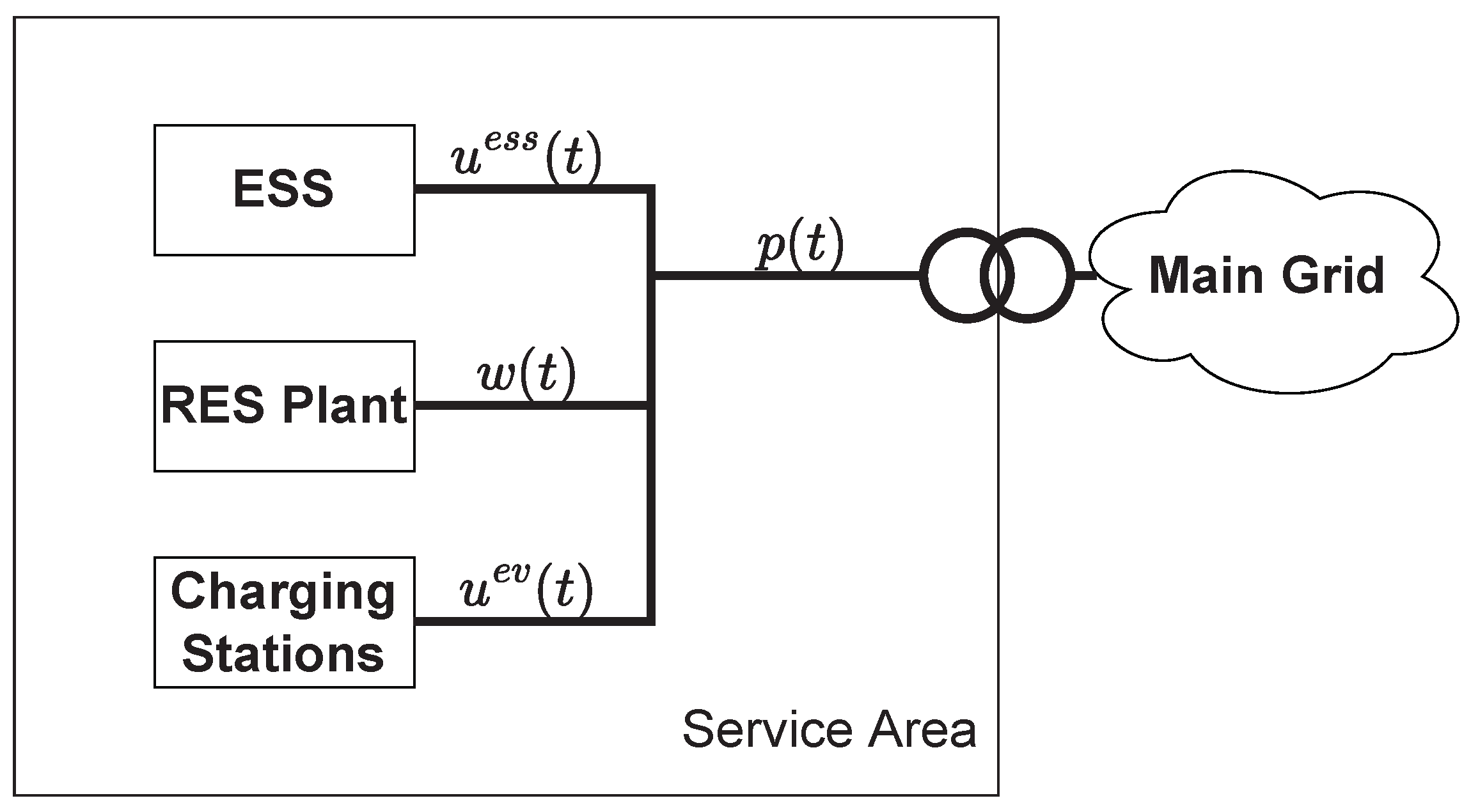
2.1. Case 1—BUS Configuration

The first configuration that has been considered for the service area is composed such as to have the charging stations, the renewable plants, and the ESS connected to the same POC to the main grid, as depicted in Figure 1.
This kind of configuration can be found in different applications, as in [18,19,20], even if in this paper a simplified version is considered. In the following, a set of equations describing the first setup is presented. The ESS dynamics in the discrete-time and considering conversion losses can be modeled as:
x ( t + 1 ) = x ( t ) + T η c h u e s s ( t ) if u e s s ( t ) 0 x ( t ) + T 1 η d i s u e s s ( t ) if u e s s ( t ) < 0 ,
where x ( t ) represents the state-of-charge (SOC) of the ESS, T represents the sampling time, u e s s ( t ) [ u m i n e s s , u m a x e s s ] represents the power absorbed/delivered by the ESS, and η c h ( 0 , 1 ) and η d i s ( 0 , 1 ) represent the charging and discharging conversion losses, respectively. Equation (1) can be rewritten by using Boolean variables α ( t ) , β ( t ) { 0 , 1 } as:
x ( t + 1 ) = x ( t ) + T u e s s ( t ) α ( t ) η c h + β ( t ) 1 η d i s ,
with additional constraints:
α ( t ) + β ( t ) 1 t ,
that ensure that α ( t ) and β ( t ) are never both equal to one at the same time, and:
β ( t ) u m i n e s s u e s s ( t ) α ( t ) u m a x e s s
to ensure that α ( t ) = 1 when u e s s ( t ) > 0 , and β ( t ) = 1 when u e s s ( t ) < 0 (notice that the maximum discharging power, u m i n e s s , is negative).
The initial state of the ESS is given by x ( t 0 ) = x 0 and the state x ( t ) is bounded by:
x m i n x ( t ) x m a x t .
The power balance equation at the POC is given by:
p ( t ) = u e s s ( t ) + u e v ( t ) w ( t ) ,
where u e v ( t ) is the power delivered to the PEVs and w ( t ) is the power produced by the Renewable Energy Sources (RES) plant installed in the service area. Additionally, the total charging power for the PEVs (i.e., u e v ( t ) ) is bounded by:
0 u e v ( t ) u ^ e v ( t ) t ,
where u ^ e v ( t ) is the cumulative power demand of the charging PEVs. The introduction of variable u e v ( t ) to control the charging power delivered to the PEVs, which may differ from the power demand, u ^ e v ( t ) , adds an additional degree of freedom to the system. Moreover, it is worth noticing that u ^ e v ( t ) and w ( t ) are considered unknown disturbances for the system, for which it is assumed that their expected values are E [ u ^ e v ( t ) ] and E [ w ( t ) ] .
In this paper, the control action (i.e., u e s s ( t ) and u e v ( t ) ) is computed by using the well-known discrete-time MPC formulation. According to the MPC technique, a new solution is computed at each time step t for a certain horizon in the future t + N T (i.e., the prediction horizon), but only the solution for the time instant t is actuated in the target system, while the other solutions for time instants [ t + T , t + N T ] are discarded. Then, the system evolves according to the control input that has been actuated and the optimization problem is computed again at the next time step by feeding it with the measurement of the new state from the system. The problem solved at each MPC iteration is as follows.
Problem 1
(Service Area Fast Charging—BUS case.). Let x ( t i ) denote the ESS SOC at time t i ; when a MPC iteration is computed, let s, q, c ( t ) , r R denote appropriate weight factors for the objective function, and let N T denote the length of the horizon with sampling time T. Then, the optimal control action is computed according to:
arg min u e v , u e s s E [ s x ( t i + N T ) x r e f 2 + + t = t i t i + ( N 1 ) T q x ( t ) x r e f 2 + c ( t ) u e v ( t ) u ^ e v ( t ) 2 + r p ( t ) 2 ]
subject to constraints (2)–(7).
Problem 1 can be rewritten, by using (6) and by isolating the unknown variables, as:
arg min u e v , u e s s { s x ( t i + N ) x r e f 2 + t = t i t i + ( N 1 ) T [ q x ( t ) x r e f 2 + c ( t ) u e v ( t ) 2 2 u e v ( t ) E [ u ^ e v ( t ) ] + E [ u ^ e v ( t ) ] 2 + + r u e s s ( t ) 2 + u e v ( t ) 2 + 2 u e s s ( t ) u e v ( t ) + 2 ( u e s s ( t ) + u e v ( t ) ) E [ w ( t ) ] + E [ w ( t ) ] 2 . }
From the objective function (8), it is possible to notice that Problem 1 can be solved by substituting E [ u ^ e v ( t ) ] and E [ w ( t ) ] to u ^ e v ( t ) and w ( t ) of the equivalent deterministic problem.

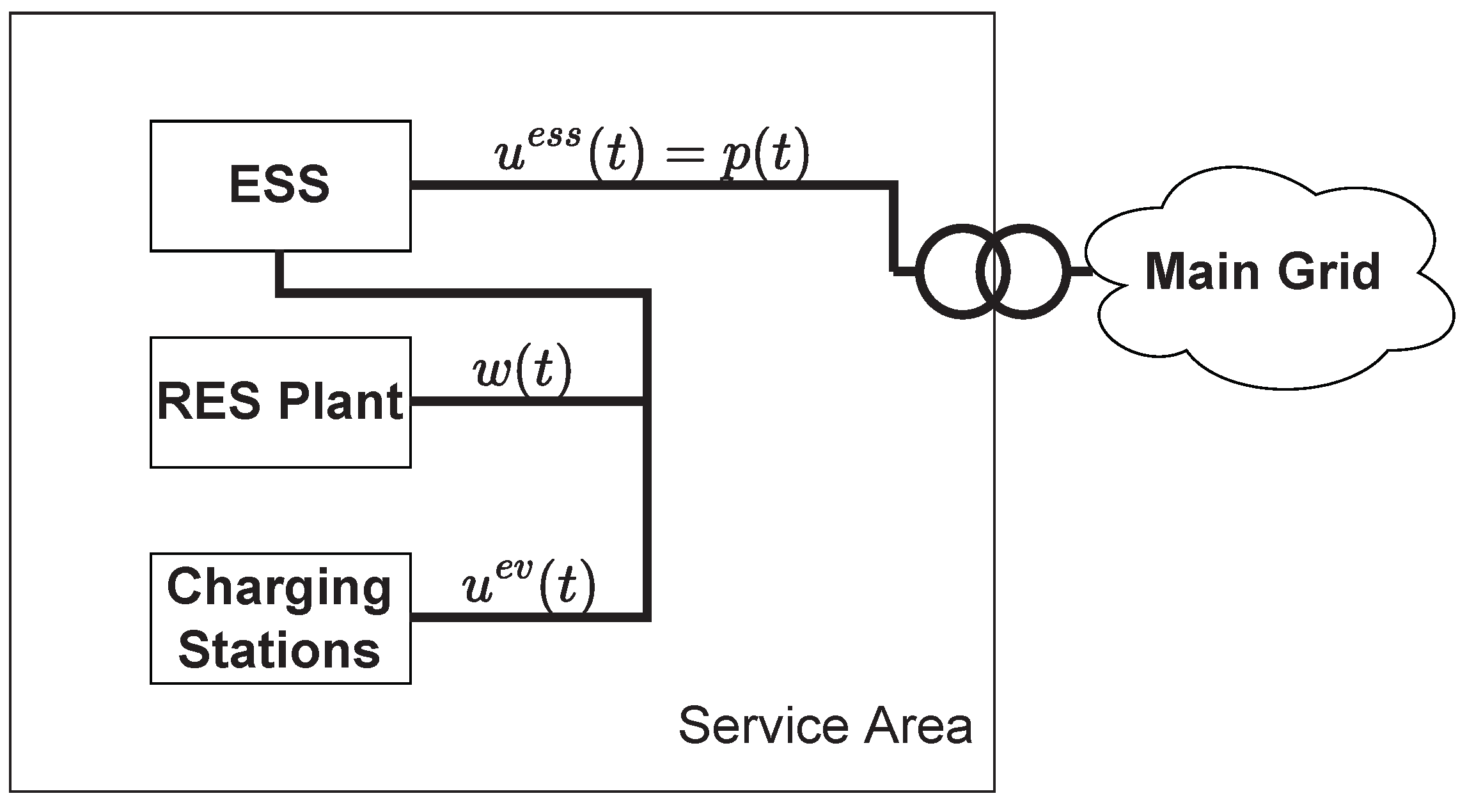
2.2. Case 2—UPS Configuration

The second configuration considered in this paper, i.e., the UPS configuration shown in Figure 2, foresees that the ESS is directly connected at the POC, and the production and consumption units are connected to the ESS. In this case, the ESS works as an energy buffer for the PEVs and RES plant.
Differently from case 1, the power balance equation at the POC (Equation (6)) becomes:
p ( t ) = u e s s ( t )
since the only device connected at the POC is the ESS itself. Moreover, since the charging PEVs and the RES plant are connected to the ESS, the ESS SOC evolves according to the total power inflow/outflow from the ESS. In particular, the new variable ρ ( t ) can be defined as:
ρ ( t ) = u e s s ( t ) u e v ( t ) + w ( t ) ,
then, Equation (1) becomes:
x ( t + 1 ) = x ( t ) + T η c h ρ ( t ) if ρ ( t ) 0 x ( t ) + T 1 η d i s ρ ( t ) if ρ ( t ) < 0 .
As in (2), it is possible to rewrite (11) as:
x ( t + 1 ) = x ( t ) + T ρ ( t ) α ( t ) η c h + β ( t ) 1 η d i s ,
with α ( t ) and β ( t ) { 0 , 1 } and additional constraints, as in Equation (3).
Constraint (4), in this case, becomes:
β ( t ) u m i n e s s ρ ( t ) α ( t ) u m a x e s s
ensuring that ρ ( t ) , i.e., the power entering/exiting the ESS, is bounded by a certain maximum and minimum power (respectively, u m a x e s s and u m i n e s s ) to ensure the safe operation of the ESS.
The remaining constraints (5) and (7) are still valid for this second setup.
As in setup 1, u ^ e v ( t ) and w ( t ) are considered as unknown disturbances for the system, and it is assumed that their expected values are E [ u ^ e v ( t ) ] and E [ w ( t ) ] .
A similar MPC approach is used to compute the control action (i.e., u e s s ( t ) and u e v ( t ) , as in setup 1), and the problem solved at the generic MPC iteration at time t i is as follows.
Problem 2
(Service Area Fast Charging—UPS case.). Let x ( t i ) the ESS SOC at time t i , when an MPC iteration is computed, let s, q, c ( t ) , and r R be the appropriate weight factors for the objective function, and let N T be the length of the horizon with sampling time T. Then, the optimal control action is computed according to:
arg min u e v , u e s s E [ s x ( t i + N T ) x r e f 2 + + t = t i t i + ( N 1 ) T q x ( t ) x r e f 2 + c ( t ) u e v ( t ) u ^ e v ( t ) ] 2 + r p ( t ) 2 ]
with constraints (5), (7), (9), (10), (12), (13).
Problem 2 can be rewritten, by using (9) and (12), and by isolating unknown variables, as follows:
arg min u e v , u e s s { s x ( t i ) + T t = t i t i + ( N 1 ) T u e s s ( t ) u e v ( t ) + E [ w ( t ) ] α ( t ) η c h + β ( t ) 1 η d i s x r e f 2 + t = t i t i + ( N 1 ) T [ q x ( t i ) + T t = t i t i + ( N 1 ) T u e s s ( t ) u e v ( t ) + E [ w ( t ) ] α ( t ) η c h + β ( t ) 1 η d i s x r e f 2 + + c ( t ) u e v ( t ) 2 2 u e v ( t ) E [ u ^ e v ( t ) ] + E [ u ^ e v ( t ) ] 2 + r ( u e s s ( t ) ) 2 } .
Similar to the BUS configuration, from the objective function (8), it is possible to notice that Problem 2 can be solved by substituting E [ u ^ e v ( t ) ] and E [ w ( t ) ] to u ^ e v ( t ) and w ( t ) of the equivalent deterministic problem.

3. Simulation Results

Three sets of simulations are proposed in this paper to validate the control algorithms presented in the previous section, and their ability to cope with unknown RES power production ( w ( t ) ) and the unknown number of fast-charging sessions (i.e., their requested power u ^ e v ( t ) ).
Moreover, different choices for the parameters of the controller will be discussed in the following, both to validate the chosen parameters and to simplify the optimization problems presented in the previous chapter. This aspect is crucial since the sampling time in the MPC framework must always be higher than the computation time of the optimization problem run at each time step, to let the control system be able to compute the next control action before the next sampling time arrives. Reducing the computation time (e.g., by moving to a simpler optimization problem to be solved at each time step) allows to reduce the sampling time of the system, thus improving the overall control performance of the MPC algorithm.

3.1. Simulation Setup

The same simulation setup has been considered for the BUS and the UPS configurations, to validate the results of the proposed control algorithms in similar situations. The service area, as depicted in Figure 1 and Figure 2, is composed by an ESS with x m a x = ( 500 M ) kWh, x m i n = ( 10 + M ) kWh, x r e f = 250 kWh, and u m a x e s s = u m i n e s s = 500 kW, by 10 fast charging stations with maximum power p m a x e v = 50 kW each (i.e., 0 u ^ e v ( t ) u ^ m a x e v , with u ^ m a x e v = 500 kW). M is a scalar value that is chosen so that M t ( E [ w ( t ) ] w ( t ) ) d t . A time span of 24 h was considered for the simulations, and the weights of the optimization problems are: q = 8 , r = 6 , and s = 2 . For the weight c, the next subsection will discuss the benefits of having a variable weight instead of a fixed value. The horizon window N has been set to 72 time steps, each one of 5 min (i.e., the sampling time of the MPC controller T). The curve w ( t ) used in the simulations below, depicted in Figure 3a, represents the typical behavior of a photovoltaic RES plant. The curve u ^ e v ( t ) used for the simulation is instead depicted in Figure 3b. In these figures, the expected values E [ w ( t ) ] and E [ u ^ e v ( t ) ] , respectively, are represented as dashed lines, together with a realization of the curves w ( t ) and u ^ e v ( t ) (solid lines). As detailed in the following, the MPC controller (Problems 1 and 2) executed at time t i knows the exact values w ( t ) and u ^ e v ( t ) for t [ t i , t i + T ) , while for the remaining time t [ t i + T , t i + N T ] , it only knows the expected values E [ w ( t ) ] and E [ u ^ e v ( t ) ] . This assumption is reasonable, since it is possible to measure the instant values of w ( t i ) and u ^ e v ( t i ) at time t i and they can be considered almost constant in the time span t [ t i , t i + T ) , since T is small.

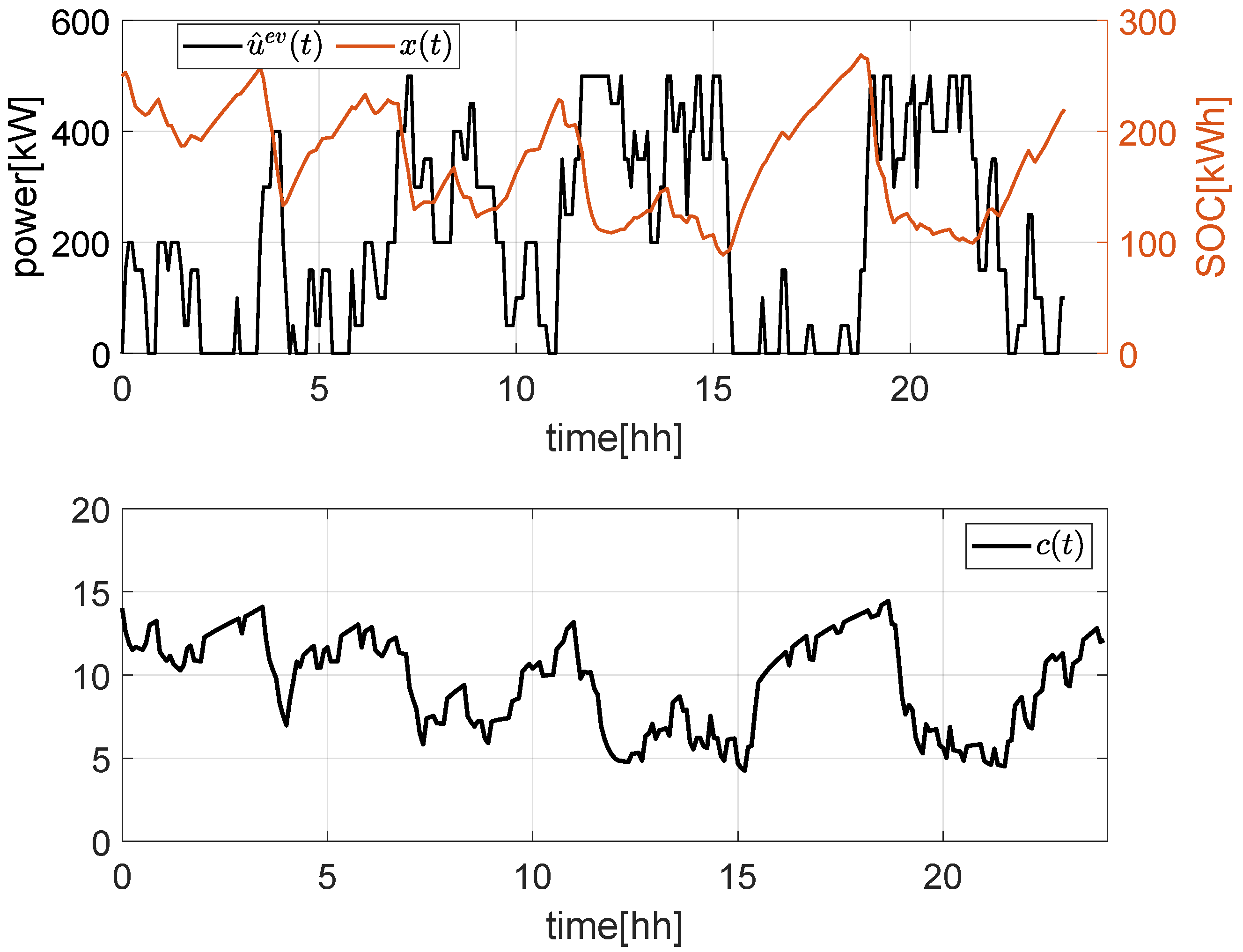
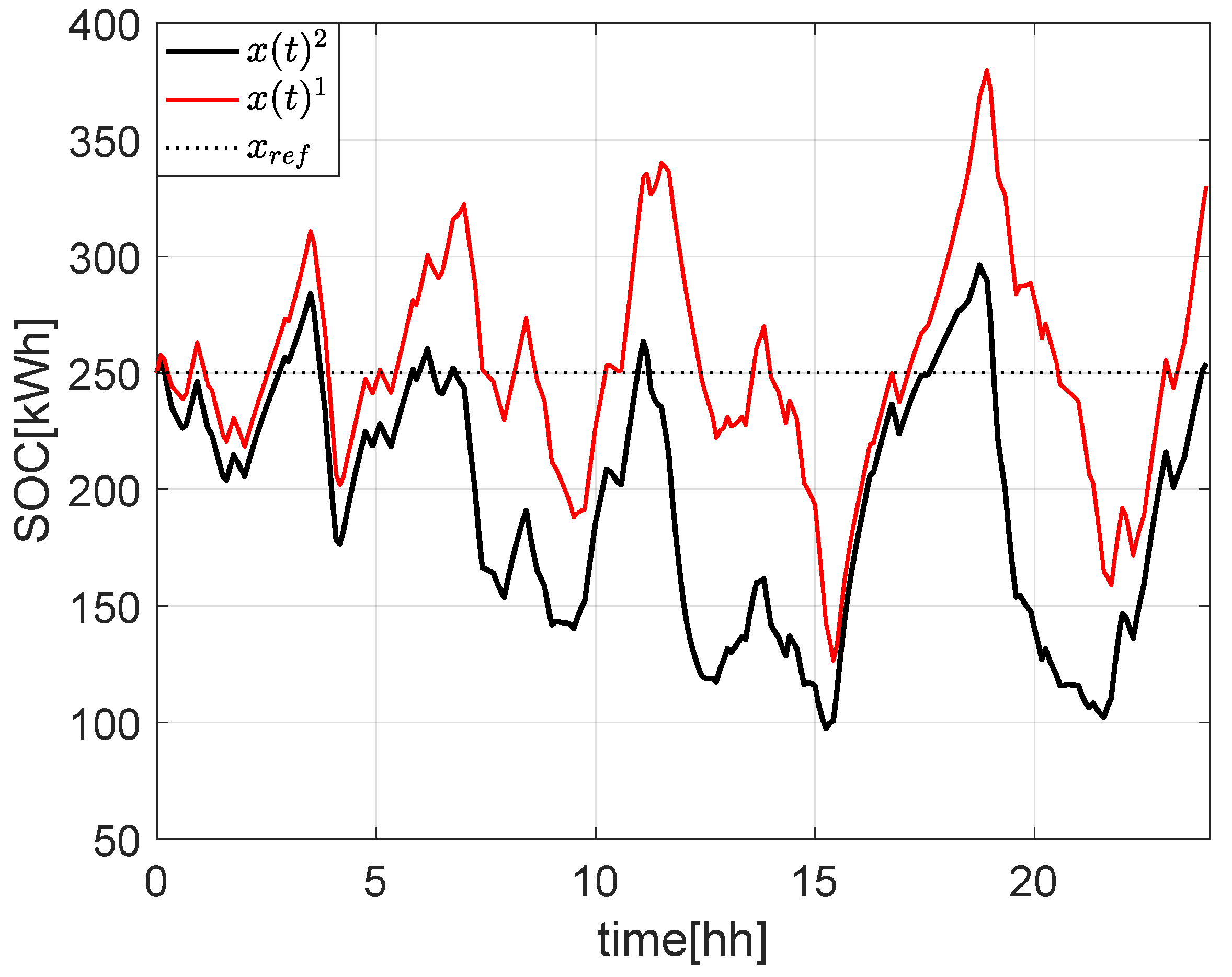
3.2. Simulation 1: Comparison between Fixed and Variable Weight for the Charging Power Tracking Term

The weight c in the objective function of Problems 1 and 2 weighs the charging power tracking term ( u ^ e v ( t ) u e v ( t ) ) 2 , which aims to compute a signal ( u e v ( t ) ) for the aggregate charging power control for the PEVs, which is as close as possible to the aggregate charging power demand u ^ e v ( t ) . By having a fixed weight c, it is not possible to model situations with high congestion in the service area, i.e., situations with a high number of charging sessions (i.e., high charging power demand u ^ e v ( t ) ) and/or ESS SOC x ( t ) far from the reference value x r e f . Indeed, in these situations, which are usually quite limited in time, the main objective of this control system—to limit the power flow at POC, thus reducing the connection fees for the service area owner—may become of higher priority than the provisioning of fast-charging services to the PEVs.
The idea is, then, to define a variable weight c ( t ) that is higher in case of no congestion in the service area (to ensure good tracking between the provided charging power and the charging power demand) and lower in case of congestion (worsening the tracking between charging power and charging power demand, but reducing the overall power p ( t ) at the POC). The proposed variable weight c ( t ) is:
c ( t ) = c ( u ^ e v ( t ) , x ( t ) ) : = h h 0 + u ^ m a x e v p m a x e v u ^ e v ( t ) p m a x e v + g x ( t ) x m a x .
It is worth noting that the weight c ( t ) is always positive, and in particular, it is never lower than h 0 , also in case of maximum congestion (i.e., all charging stations occupied and requesting full power, and 0% ESS SOC). This indicates that the tracking term, even with a lower weight, is always preserved in the objective function of Problems 1 and 2.
In the following simulations, the weights g = 0.15 , h = 0.5 and h 0 = 3 have been chosen, leading to c ( t ) as in Figure 4.
Figure 5 shows the action of fixed c or variable c ( t ) on control variable u e v ( t ) . As the congestion is higher (e.g., from 5 h to 10 h, from 10 h to 15 h, and around 20 h), the cost c ( t ) is lower, leading to a higher mismatch between u ^ e v ( t ) and the control variable u e v ( t ) than in the case with fixed c (red line). This is also reflected in Figure 6, where the power at POC is almost the same in case of low congestion, while it is definitely lower in case of high congestion. Given the control objectives presented in the previous sections, the case with variable c ( t ) is, then, definitely preferable with respect to the case with fixed c. Moreover, from Figure 7, which represents the evolution of the ESS SOC (black line for variable c ( t ) and red line for fixed c), it is possible to notice that in both cases, there is no risk for saturation in the ESS.

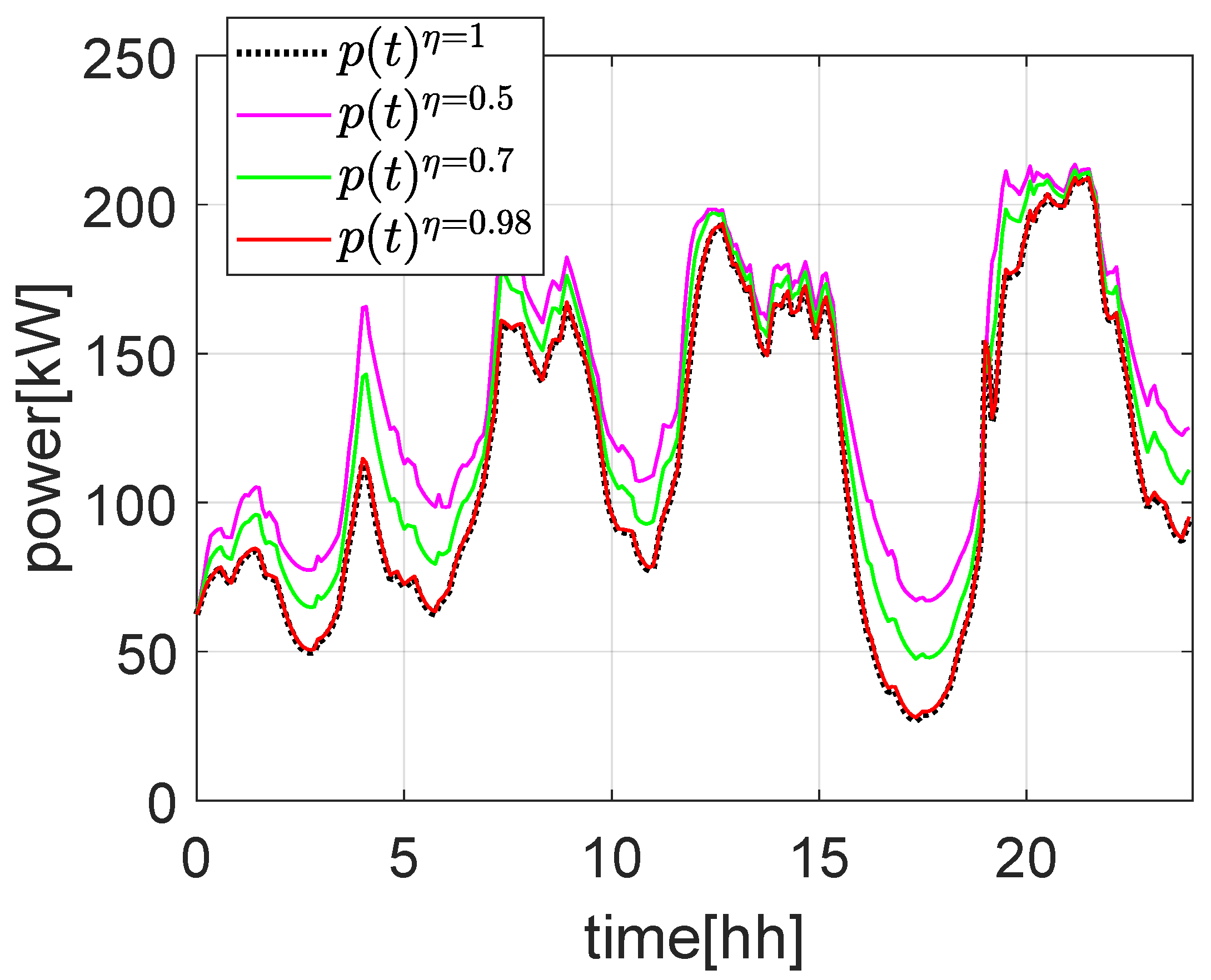
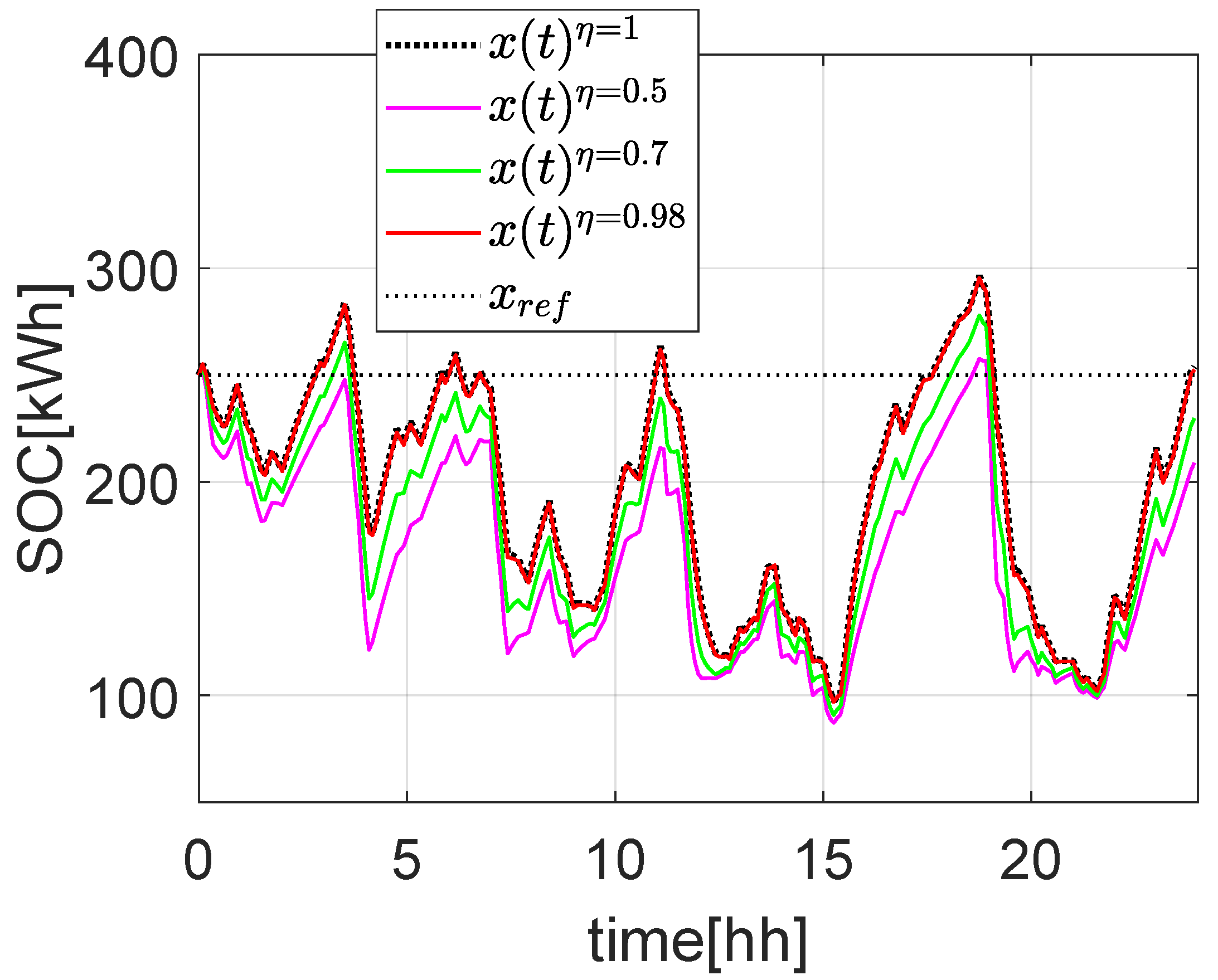
3.3. Simulation 2: Effects of Power Losses

In the formalization of Problems 1 and 2, the constraints (2) and (12) represent the evolution of the ESS SOC by considering power losses η c h for charging and η d i s for discharging. The next set of simulations aims to show that an equivalent problem not including the loss terms introduces only a small amount of error, compared to the error introduced by moving from a deterministic to a stochastic formulation. On the contrary, the benefits of removing charging and discharging losses make Problems 1 and 2 much more simple to solve, given the fact that all the Boolean variables are removed from the problems, so a simpler Quadratic Programming solver can be used instead of a Mixed-Integer Quadratic Programming one.
Figure 8 and Figure 9 show the evolution of the deterministic problem (i.e., w ( t ) = E [ w ( t ) ] and u ^ e v ( t ) = E [ u ^ e v ( t ) ] ) with different values of charging and discharging power losses η c h and η d i s . Without loss of generality, for this set of simulations, we chose η c h = η d i s = η . As is possible to note from Figure 8, the introduction of power losses (even of a big entity, like with η = 0.7 ) introduces a minimal error (around 10%) on the power at POC and on the ESS SOC (Figure 9). By considering normal power conversion losses (which are usually around 1–2%), the difference with respect to the case without losses is almost invisible. This indicates that it is possible to simplify the mathematical formulation of Problems 1 and 2 by removing constraint (2) and (12), respectively, by replacing them with the following simpler constraints:
x ( t + 1 ) = x ( t ) + T p ( t )
x ( t + 1 ) = x ( t ) + T ρ ( t )
respectively, for Problems 1 and 2, by removing the Boolean variables α and β , which made the problems mixed-integer.
Moreover, the error introduced by removing such Boolean variables (i.e., by not modeling power conversion losses in the ESS SOC dynamics) is expected to be considerably lower than the error introduced by the non-determinism of Problems 1 and 2.

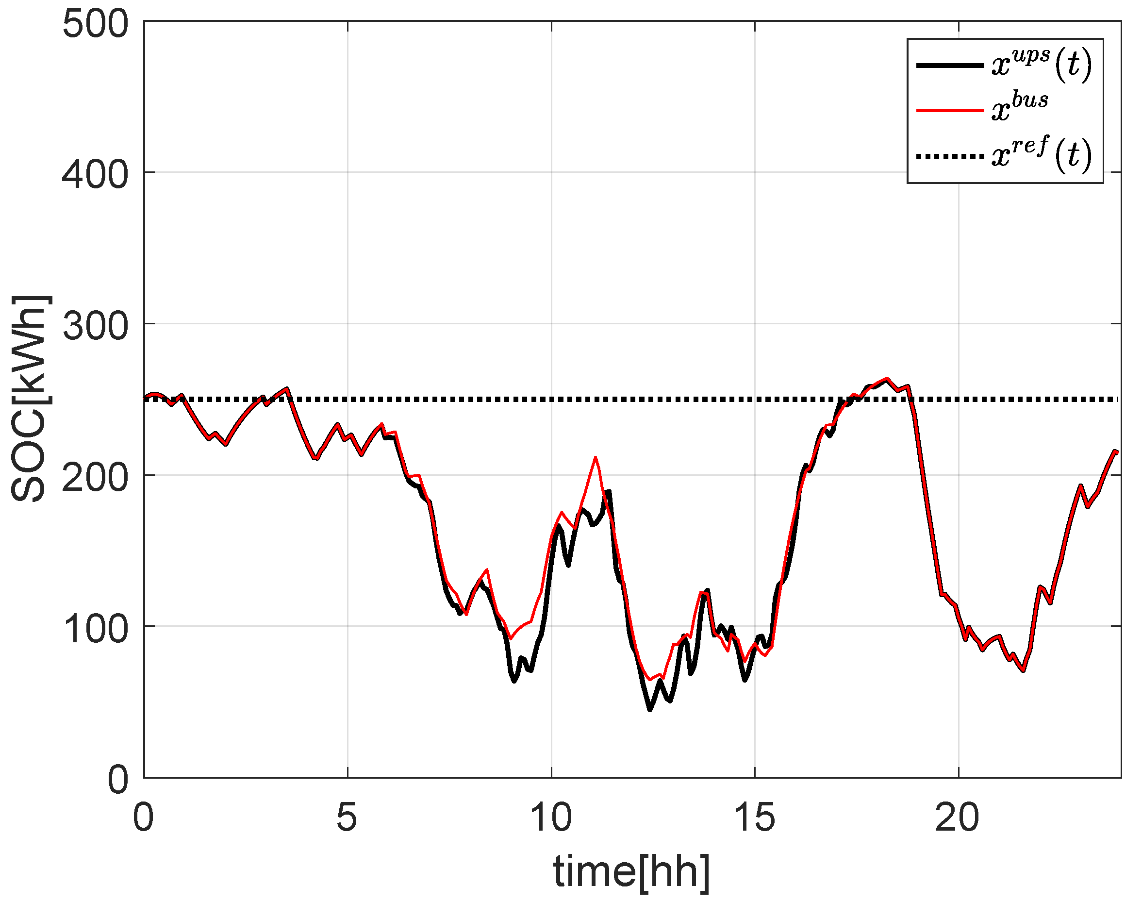
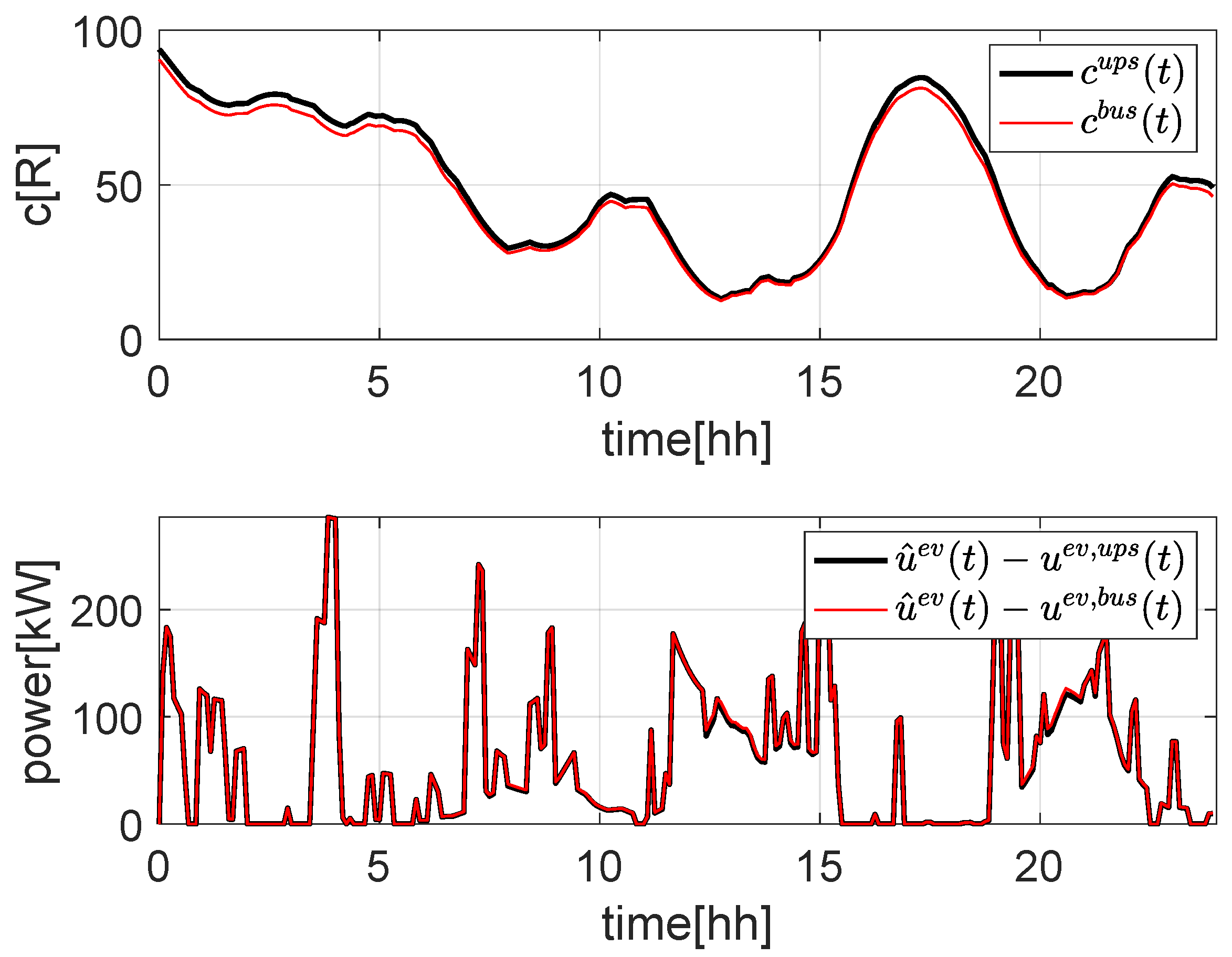
3.4. Simulation 3: Comparison between BUS and UPS Configuration in Case of Uncertainties

In this subsection, the comparison of case 1 (BUS) and case 2 (UPS) will be analyzed according to the formulation of Problems 1 and 2 with constraints (16) and (17) (i.e., without considering power losses).
As is possible to note from Figure 10, the BUS configuration suffers from the uncertainties of w ( t ) on power at POC p ( t ) , while from Figure 11, it is possible to note that the effects of uncertainties affect the ESS SOC x ( t ) . This behavior is as expected since in the BUS configuration the RES plant is directly connected to the POC, while in the UPS configuration, it is connected to the ESS.
It is important to note that the uncertainties on u ^ e v ( t ) do not affect either p ( t ) or x ( t ) . This is due to the fact that u ^ e v ( t ) is not directly applied to the charging PEV, but the latter is controlled by the control variable u e v ( t ) . This means that any uncertainties on u ^ e v ( t ) directly reflect on the end-user charging power rather than on the power at the POC or the ESS SOC.
As is possible to see from Figure 12, the power profile delivered to the PEVs slightly changes from the BUS to the UPS configurations, due to the fact that the cost c ( t ) (which weighs the power tracking term) also depends on x ( t ) , which is subject to the uncertainties of w ( t ) for the UPS configuration. A detailed comparison of the power profiles u e v ( t ) in the two configurations can be found in Figure 13, where it is possible to see that the UPS configuration provides slightly more power to the charging PEVs with respect to the BUS configuration. Moreover, the UPS configuration benefits of decoupling the power profile at the POC p ( t ) from the uncertainties.

4. Conclusions

In this paper, a stochastic model predictive control for a service area providing the electric vehicles fast charging service has been presented. A key feature of the proposed control is the tracking of an uncertain reference for charging in minimum time, which is dynamically relaxed for the mitigation of congestion. The comparison of control performances between the BUS and UPS infrastructure setups has revealed a substantial equivalence between them in relation to their ability to withstand the effect of uncertain signals, while confirming the effectiveness of the congestion mitigation strategy in both cases. It is worth noting that uncertainty affects different portions of the two setups, an aspect that constitutes a significant difference between them. In general, the UPS configuration benefits from the fact that any uncertainties affect only the state of the ESS, which is an internal variable of the system, without affecting the power at the POC. In practice, the choice of one setup over the other should also consider an in-depth analysis of other key electrical and economic aspects, in particular the ESS size (which in the UPS configuration should be enough to provide the full power demand of the PEVs), degradation, and expected lifetime, which may significantly affect capital and operational expenditures.
Future works will consider in detail the introduction of chance constraints in the problem formalization, also in the context of a continuous-time framework.

Author Contributions

Conceptualization, A.D.G., E.D.S. and F.L.; methodology, A.D.G., E.D.S. and F.L.; software, L.F. and S.F.; validation, A.D.G., E.D.S., L.F., S.F. and F.L.; writing—original draft preparation, E.D.S., A.D.G. and F.L.; writing—review and editing, A.D.G., F.L., L.F. and S.F. All authors have read and agreed to the published version of the manuscript.

Funding

This work has been carried out in the framework of the 5G-SOLUTIONS project, which has received funding from the European Union’s Horizon 2020 research and innovation programme under grant agreement No 856691. The content of this paper reflects only the authors’ view; the EU Commission/Agency is not responsible for any use that may be made of the information it contains.

Institutional Review Board Statement

Not applicable.

Informed Consent Statement

Not applicable.

Data Availability Statement

Not applicable.

Conflicts of Interest

The authors declare no conflict of interest.

Abbreviations

The following abbreviations are used in this manuscript:
ESSEnergy Storage System
MPCModel Predictive Control
PEVPlug-in Electric Vehicles
POCPoint of Connection
PMPPontryagin Minimum Principle
RESRenewable Energy Sources
SOCState-of-Charge

References

  1. Szumska, E.M. Electric Vehicle Charging Infrastructure along Highways in the EU. Energies 2023, 16, 895. [Google Scholar] [CrossRef]
  2. Negarestani, S.; Fotuhi-Firuzabad, M.; Rastegar, M.; Rajabi-Ghahnavieh, A. Optimal sizing of storage system in a fast charging station for plug-in hybrid electric vehicles. IEEE Trans. Transp. Electrif. 2016, 2, 443–453. [Google Scholar] [CrossRef]
  3. Kim, N.; Cha, S.; Peng, H. Optimal control of hybrid electric vehicles based on Pontryagin’s minimum principle. IEEE Trans. Control Syst. Technol. 2010, 19, 1279–1287. [Google Scholar]
  4. Heymann, B.; Bonnans, J.F.; Martinon, P.; Silva, F.J.; Lanas, F.; Jiménez-Estévez, G. Continuous optimal control approaches to microgrid energy management. Energy Syst. 2018, 9, 59–77. [Google Scholar] [CrossRef] [Green Version]
  5. Zheng, C.; Li, W.; Liang, Q. An energy management strategy of hybrid energy storage systems for electric vehicle applications. IEEE Trans. Sustain. Energy 2018, 9, 1880–1888. [Google Scholar] [CrossRef]
  6. Kou, P.; Feng, Y.; Liang, D.; Gao, L. A model predictive control approach for matching uncertain wind generation with PEV charging demand in a microgrid. Int. J. Electr. Power Energy Syst. 2019, 105, 488–499. [Google Scholar] [CrossRef]
  7. Kou, P.; Liang, D.; Gao, L.; Gao, F. Stochastic coordination of plug-in electric vehicles and wind turbines in microgrid: A model predictive control approach. IEEE Trans. Smart Grid 2015, 7, 1537–1551. [Google Scholar] [CrossRef]
  8. Liberati, F.; Di Giorgio, A.; Koch, G. Optimal stochastic control of energy storage system based on pontryagin minimum principle for flattening pev fast charging in a service area. IEEE Control Syst. Lett. 2021, 6, 247–252. [Google Scholar] [CrossRef]
  9. Giorgio, A.D.; Atanasious, M.M.H.; Guetta, S.; Liberati, F. Control of an Energy Storage System for Electric Vehicle Fast Charging: Impact of Configuration Choices and Demand Uncertainty. In Proceedings of the 2021 IEEE International Conference on Environment and Electrical Engineering and 2021 IEEE Industrial and Commercial Power Systems Europe (EEEIC / I&CPS Europe), Bari, Italy, 7–10 September 2021; pp. 1–6. [Google Scholar] [CrossRef]
  10. Ding, X.; Zhang, W.; Wei, S.; Wang, Z. Optimization of an energy storage system for electric bus fast-charging station. Energies 2021, 14, 4143. [Google Scholar] [CrossRef]
  11. Sun, B. A multi-objective optimization model for fast electric vehicle charging stations with wind, PV power and energy storage. J. Clean. Prod. 2021, 288, 125564. [Google Scholar] [CrossRef]
  12. Leonori, S.; Rizzoni, G.; Mascioli, F.M.F.; Rizzi, A. Intelligent energy flow management of a nanogrid fast charging station equipped with second life batteries. Int. J. Electr. Power Energy Syst. 2021, 127, 106602. [Google Scholar] [CrossRef]
  13. Kucevic, D.; Englberger, S.; Sharma, A.; Trivedi, A.; Tepe, B.; Schachler, B.; Hesse, H.; Srinivasan, D.; Jossen, A. Reducing grid peak load through the coordinated control of battery energy storage systems located at electric vehicle charging parks. Appl. Energy 2021, 295, 116936. [Google Scholar] [CrossRef]
  14. Huang, Y.; Yona, A.; Takahashi, H.; Hemeida, A.M.; Mandal, P.; Mikhaylov, A.; Senjyu, T.; Lotfy, M.E. Energy management system optimization of drug store electric vehicles charging station operation. Sustainability 2021, 13, 6163. [Google Scholar] [CrossRef]
  15. Chen, X.; Pang, Z.; Zhang, M.; Jiang, S.; Feng, J.; Shen, B. Techno-economic study of a 100-MW-class multi-energy vehicle charging/refueling station: Using 100% renewable, liquid hydrogen, and superconductor technologies. Energy Convers. Manag. 2023, 276, 116463. [Google Scholar] [CrossRef]
  16. Parlikar, A.; Schott, M.; Godse, K.; Kucevic, D.; Jossen, A.; Hesse, H. High-power electric vehicle charging: Low-carbon grid integration pathways with stationary lithium-ion battery systems and renewable generation. Appl. Energy 2023, 333, 120541. [Google Scholar] [CrossRef]
  17. Kumar, N.; Kumar, T.; Nema, S.; Thakur, T. A comprehensive planning framework for electric vehicles fast charging station assisted by solar and battery based on Queueing theory and non-dominated sorting genetic algorithm-II in a co-ordinated transportation and power network. J. Energy Storage 2022, 49, 104180. [Google Scholar] [CrossRef]
  18. Tan, H.; Chen, D.; Jing, Z. Optimal Sizing of Energy Storage System at Fast Charging Stations under Electricity Market Environment. In Proceedings of the 2019 IEEE 2nd International Conference on Power and Energy Applications (ICPEA), Singapore, 27–30 April 2019. [Google Scholar] [CrossRef]
  19. Comitato Elettrotecnico Italiano. CEI-016-Reference Technical Rules for the Connection of Active and Passive Consumers to the HV and MV Electrical Networks of Distribution Company, v1. 2020. Available online: https://www.ceinorme.it/doc/norme/016021_2019/0-16_2019.pdf (accessed on 28 December 2022).
  20. Comitato Elettrotecnico Italiano. CEI-021-Reference Technical Rules for the Connection of Active and Passive Users to the LV Electrical Utilities, v1. 2020. Available online: https://www.ceinorme.it/doc/norme/18309.pdf (accessed on 28 December 2022).
Figure 1. Setup of case 1—BUS.
Energies 16 01348 g001
Figure 2. Setup of case 2—UPS.
Energies 16 01348 g002
Figure 3. The curve w ( t ) and u ^ e v ( t ) chosen for the simulations. The black line represents the expected values of E [ w ( t ) ] and E [ u ^ e v ( t ) ] in (a) and (b), respectively; the red line represents a realization of the actual curve w ( t ) and u ^ e v ( t ) in (a) and (b), respectively. (a) Curve w ( t ) chosen for the simulations; (b) The curve u ^ e v ( t ) chosen for the simulations.
Energies 16 01348 g003
Figure 4. Evolution of cost c ( t ) based on PEVs’ power demand and ESS SOC.
Energies 16 01348 g004
Figure 5. Evolution of mismatch between power demand for charging PEVs ( u ^ e v ( t ) ) and power delivered to PEVs ( u e v ( t ) ). · 1 is computed with fixed c = 15 ; · 2 is computed with c ( t ) , as in (15).
Energies 16 01348 g005
Figure 6. Power evolution at POC. p ( t ) 1 is computed with fixed c = 15; p ( t ) 2 is computed with c(t), as in (15).
Energies 16 01348 g006
Figure 7. ESS SOC evolution. x ( t ) 1 is computed with fixed c = 15; x ( t ) 2 is computed with c(t), as in (15).
Energies 16 01348 g007
Figure 8. Power evolution at POC with different power conversion losses factors η { 0.5 , 0.7 , 0.98 , 1 } .
Energies 16 01348 g008
Figure 9. ESS SOC evolution with different power conversion losses factors η { 0.5 , 0.7 , 0.98 , 1 } .
Energies 16 01348 g009
Figure 10. Evolution of power at POC in case of uncertainties for BUS (red) and UPS (black) configurations.
Energies 16 01348 g010
Figure 11. ESS SOC evolution in case of uncertainties for BUS (red) and UPS (solid black) configurations.
Energies 16 01348 g011
Figure 12. Comparison between power delivered to PEVs (bottom) and variable cost c ( t ) (top) for BUS and UPS configurations.
Energies 16 01348 g012
Figure 13. Difference between power provided to PEVs in BUS and UPS configurations.
Energies 16 01348 g013
Table 1. Nomenclature used in the paper.
SymbolExplanation
gConstant used to define weight c in (15).
hConstant used to define weight c in (15).
h 0 Constant used to define weight c in (15).
NLength [number of sampling intervals] of the MPC prediction horizon.
p ( t ) Power [kW] flowing at the POC during time interval t.
p m a x e v Maximum power [kW] of a high-power charging station.
qWeight of the state term in the objective function.
rWeight of the power term in the objective function.
sWeight of the control term in the objective function.
tGeneric time interval.
t 0 Initial time interval.
TSampling time.
u e s s ( t ) ESS charging/discharging power [kW] during interval t.
u m a x e s s Maximum ESS charging power [kW].
u m i n e s s Maximum ESS discharging power [kW].
u e v ( t ) Total power [kW] delivered to the PEVs during interval t.
u ^ e v ( t ) Total power [kW] demand from the PEVs during interval t.
u ^ m a x e v Maximum aggregated power demand [kW] for charging stations.
w ( t ) RES power [kW] produced during interval t.
x ( t ) ESS SOC [kWh] at the beginning of time interval t.
x 0 ESS initial SOC [kWh].
x m i n , x m a x respectively, minimum and maximum possible ESS SOC [kWh].
x r e f Reference ESS SOC [kWh].
α t Boolean variable equal to one if the ESS recharges during time interval t.
β t Boolean variable equal to one if the ESS discharges during time interval t.
η c h , η d i s The ESS charging and discharging conversion losses, respectively.
ρ ( t ) Total power [kW] entering or exiting the ESS at time t in the UPS configuration.
Disclaimer/Publisher’s Note: The statements, opinions and data contained in all publications are solely those of the individual author(s) and contributor(s) and not of MDPI and/or the editor(s). MDPI and/or the editor(s) disclaim responsibility for any injury to people or property resulting from any ideas, methods, instructions or products referred to in the content.

