Abstract
The smart grid concept is introduced to accelerate the operational efficiency and enhance the reliability and sustainability of power supply by operating in self-control mode to find and resolve the problems developed in time. In smart grid, the use of digital technology facilitates the grid with an enhanced data transportation facility using smart sensors known as smart meters. Using these smart meters, various operational functionalities of smart grid can be enhanced, such as generation scheduling, real-time pricing, load management, power quality enhancement, security analysis and enhancement of the system, fault prediction, frequency and voltage monitoring, load forecasting, etc. From the bulk data generated in a smart grid architecture, precise load can be predicted before time to support the energy market. This supports the grid operation to maintain the balance between demand and generation, thus preventing system imbalance and power outages. This study presents a detailed review on load forecasting category, calculation of performance indicators, the data analyzing process for load forecasting, load forecasting using conventional meter information, and the technology used to conduct the task and its challenges. Next, the importance of smart meter-based load forecasting is discussed along with the available approaches. Additionally, the merits of load forecasting conducted using a smart meter over a conventional meter are articulated in this paper.
1. Introduction
Globally, the demand of electricity is increasing day by day. The growing use of electricity has prompted multiple agencies to implement a variety of strategies for maximizing its efficiency like: efficient use of fuels and raw materials during generation, input of organic and inorganic wastes into boilers, reducing auxiliary power consumption, the intelligent switching of domestic loads in the distribution network, continuously monitoring the reduction of power loss in transmission and distribution systems, utilizing energy-efficient equipment, educating society about better load optimization, etc. Based on the above discussion, one step would be to predict the future load for each type of consumer (domestic, commercial, and industrial). For this reason, researchers are concentrating more on load forecasting. The load forecasting technique involves estimating future loads using historical and present data. In smart grid, the forecasting of loads is done by considering the power consumption by users and the power produced by all types of generations (renewable and non-renewable) with the help of smart energy meters, as shown in Figure 1. Moreover, load forecasting is becoming more difficult these days due to two reasons: firstly, due to the privatization and deregulation of distribution companies/power industries in many countries, the consumer is free to select any electricity provider of their choice among the other providers [1,2,3]. Hence, a consumer will always choose a supplier whose cost is beneficial to them in their case. In this scenario, forecasters face challenges. Secondly, due to the availability of renewable sources like solar and wind power, their uncertainty has been increased due to their inconsistent behavior [1,2,3,4,5,6,7,8,9]. In [4,5,6,7,8,9], the authors stated that due to the inherent variability of renewable resources like solar and wind energy, there is uncertainty in the consumer demand. A rapid penetration of renewable energy sources with high variability and uncertainty presents new challenges to the operation of power systems. Due to random fluctuations in weather condition, the RES may suffer from uncontrollable generation. Energy produced by user-owned generators like PV and wind power is measured with dedicated meters. Two levels of metering are used in these generation plants, one installed at the point of common coupling, which is located at the power control center end (PCC) for energy exchange, and the other installed at the user-owned generator end for measuring the actual power produced. As a result, the data regarding the actual load could be reconstructed as a net of power data, and these data could then be considered for load forecasting. In contrast to this, Kaur et al. [10] presented a load forecasting scheme based on net power. Here, the forecasting of solar or wind energy is done separately, and the forecasting of load is done separately. Then, solar/wind forecasting and load forecasting are integrated to provide a net load forecast. It should be noted that inadequate forecasting may result in an unpredicted increase in operating cost due to the continuous operation of heavily loaded generators and an inappropriate capacity of reserve allocation [11].
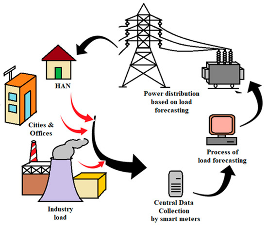
Figure 1.
Process of load forecasting in a smart grid.
In order to maintain a precise forecast of energy consumption, smart sensors/smart meters (SMs) are a must for a smart grid system. The data obtained from these SMs are collected in terms of voltage, current, both active and reactive power, power factor, and energy. These data can be stored in a central server or can be streamed in real-time. As the internet of things (IoT) communicates and stores data in a defined storage facility, it plays a crucial role in data collection and analysis [12]. Many different mediums can be used to transfer data, such as Wi-Fi, Bluetooth, Global System for Mobile communication (GSM), powerline carriers, fiber optics, etc. As part of an IoT, wireless technology is also used to gather data without human intervention. Thus, these data may help in the prediction of load in a smart grid system. Forecasting household load is difficult because of extreme system volatility resulting from the many interconnected components. Load forecasting relies on a variety of factors, such as weather conditions, wind speed, weekdays or weekends, normal days or holidays, festival days, availability of loads, etc. In order to predict load accurately, alternative techniques are needed not only because of new technologies, but also because of increasing load demands, changing consumption patterns, and rapid changes in lifestyles [13]. To forecast the load, various techniques, such as decision tree, linear regression, support vector machine, random forest, gradient boosting regression, neural network, deep learning, and many more methods, are used. Hence, in the recent scenario, the machine learning (ML)-based load forecasting is widely used by researchers.
In smart grid, due to the presence of a large number of users, the complexity of load forecasting for multiple time series can be seen [14]. As a result, two scenarios are defined: (1) training one single model for a single time series with separately learned parameters, referred to as local method, and (2) training one single model that is learned from all available time series, which is referred to as global method. In recent years, global methods have been used more often than local methods due to less overfitting [14]. A local method is mostly a statistical method, whereas a global method can be both statistical and machine learning [15,16].
2. Load Forecasting Category
Based on the time horizon, load forecasting in smart grid is classified into four categories. A description of each category can be found in Table 1.

Table 1.
Load forecasting categories based on time horizon and applications.
2.1. Very Short-Term Load Forecasting (VSTLF)
In VSTLF, the load forecasting is performed for a very short duration which ranges from a few minutes to an hour [17,18,19,20,21,22,23]. VSTLF is used for the real-time scheduling of generation, load frequency control, and resource dispatch [17,22]. It also plays an important role in auction-based electricity markets [20]. Various power networks, including those of Great Britain, China, and ISO New England, use VSTLF [17,18,22].
2.2. Short-Term Load Forecasting (STLF)
In STLF, load forecasting is performed for a short duration, i.e., from an hour to few days [13,24,25,26]. STLF can play an important role in any organization, planning for the proper load flow and avoiding the condition of overloading in the system [27]. In large-scale applications, such as where one country or group of nations (like the European Union) share a single power grid, the STLF plays a crucial role in making decisions regarding load [28].
2.3. Medium-Term Load Forecasting (MTLF)
In this type, the forecasting is performed for a duration ranging from a few days to several months to a year, as defined in [24,29,30]. MTLF is useful for planning and scheduling the preventive maintenance of unit and allows the organization to plan for raw material and fuel procurement [27].
2.4. Long-Term Load Forecasting (LTLF)
In LTLF, forecasting is performed for a duration ranging from one year to several years. Long-term forecasting accuracy is highly dependent on other variables such as weather [24,31]. LTLF is used for any organization to plan for their unit expansion or any major equipment installation [15].
3. Key Performance Indicators (KPI) for Load Forecasting
Whenever there is an error in load forecasting, the electricity suppliers may have to endure high production costs for electricity and sometimes they may be forced to go out of business because of a system failure causing a blackout [32]. It is, therefore, necessary to forecast accurately to enhance the system’s reliability and ensure uninterrupted power production. Hence, to measure the accuracy of any load forecasting technique, various KPIs are identified, which are describes as follows [20,26]:
3.1. Mean Absolute Error (MAE)
This can be calculated by the mean of the absolute error, where error () may be defined as the difference of the forecasted value () and the actual value (), as seen in Equation (1). Since the calculated error may be a negative or a positive value, the absolute value is used for MAE, which can be calculated using Equation (2).
3.2. Mean Absolute Percentage Error (MAPE)
MAPE is the division of the sum of all individual absolute errors and the actual value. It is calculated by the formula seen in Equation (3).
3.3. Root Mean Square Error (RMSE)
For RMSE, first we need to calculate the mean squared error (MSE) using Equation (4). Then, the square root of the average squared error is estimated using Equation (5).
3.4. Root Relative Squared Error (RRSE)
RRSE is the total squared error relative to the errors which have been formed if the forecasting is the average of the absolute value [14]. In other terms, RRSE is the square root of the ratio of the sum of the squared error of the forecasted and actual values to sum of the squared error of the average value and actual value. The relation for RRSE is seen in Equation (6).
where is the average of the actual value.
3.5. Coefficient of Variation (CV)
Coefficient of variation is calculated by the ratio of the predicted error standard deviation to the mean of the actual value or, in short, it is the ratio of RMSE to the mean of the actual value (), as mentioned in Equations (7) and (8) [33].
4. Data Pre-Processing
In smart grid, the data are collected through smart meters installed at the consumer’s end, the distribution transformer end, the substation end, and the generation end. In accordance with the method used, different datasets are collected from smart meters over different time horizons (e.g., 15 min, 30 min, 1 h, 1 day, 1 month, and 1 year). However, when compiling the dataset, it is not necessary to obtain the complete data at each time point; sometimes there may be missing data in the dataset for any duration, sometimes there may be outliers which overshoot or undershoot the dataset, and sometimes there is huge elimination of the dataset due to technical reasons. Therefore, in order to pre-process the dataset, various methods such as elimination, interpolation, and noise extraction are employed (Figure 2).
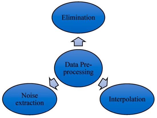
Figure 2.
Data pre-processing methods.
4.1. Elimination
In the elimination method, the user has huge unrecorded/missing data which are excluded from load forecasting considerations [32]. Furthermore, if there is a big loss of data in the dataset, then this loss of data is also eliminated from the dataset as well. If this is not conducted, then it may affect the accuracy of forecasting.
4.2. Interpolation
During the process of collecting the data, there are certain times when we may not acquire the values in between two data. Therefore, the missing data are interpolated over these single missing values. Hence, interpolation is a process of filling in missing data by interpolating the previous and next values of the missing value [34,35]. Equation (9) represents the formula of interpolation.
where is the missing value, is previous value to , and is next value to . , , and are the time of data with respect to ,, and .
4.3. Noise Extraction
Since the data are exported from the server, they contain a wide variety of noise which needs to be removed before the load forecasting model can be constructed, to ensure accurate predictions. The noises are in the terms of negative load values and some random codes [36].
4.4. Imputation
Imputation methods are most commonly used in statistics in order to overcome the problem of missing data with a substitute value [37]. In general, there are two types: single and multiple imputations. In single imputation, each missing value is replaced by a single value. In contrast, in multiple imputation, certain rules are applied to substitute the missing value [38]. Moreover, the method of imputation can further be classified as maximum likelihood imputation (MLI) methods and machine learning (ML)-based methods [39]. The MLI contains expected maximization, multiple imputation, and Bayesian principal component analysis. Additionally, the ML-based methods involve imputation with K-nearest neighbor (KNN), weighted imputation with KNN, K-means clustering imputation, imputation with fuzzy K-means clustering, SVM imputation, singular value decomposition imputation, local least square imputation, etc. [39].
5. Process of Load Forecasting
Generally, the process of forecasting load is the same for all the categories, as well as all the methods. The process of load forecasting has different steps, as shown in Figure 3.
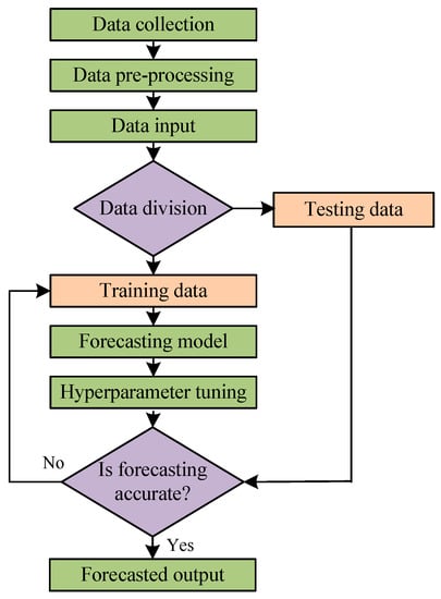
Figure 3.
Process flow diagram of load forecasting.
5.1. Data Collection
In order to forecast load, the first requirement is to collect the data. The data can be collected in various ways for load forecasting, such as manually taking the data at the customer end or at the distribution transformer end, collecting recorded data through smart meters, collecting data from the main server, and sometimes taking data that are already recorded and filed. In order to forecast load, it is obviously necessary to have historical load data, but weather-related data such as temperature-, humidity-, solar radiation-, wind speed-, and different events-related load data such as festivals, holidays, special occasions, etc., are also collected through various methods at different timelines.
5.2. Data Pre-Processing
It has already been discussed in Section 4 that the collected data are the raw data with missing values, outliers, and noises, which cannot be fed directly into forecasting models. In order to acquire authentic data, they need to be filtered out and pre-processed. There are three methods used for pre-processing: elimination, interpolation, and noise extraction [13,17].
5.3. Data Input
Pre-processed data are used as input to load forecasting models and are used to train the models. There are cases when the whole set of data is not used as input in a model. The datasets are clustered into different subgroups based on similar patterns of load. Afterwards, each cluster is trained to create an accurate forecasting model [23,36,40,41,42].
5.4. Data Division
To begin the load forecasting process, data must be divided into two parts, training and testing. Datasets are divided according to a ratio determined by the person performing the forecasting. In most cases, 70–80% of the dataset is used to train the forecasting model, whereas during the testing phase, the remaining 20–30% is used to validate and authenticate it [13,17,23,43,44]. It is necessary to divide datasets into training and testing in order to avoid overfitting. Additionally, the training data is further divided into two subsets, one known as the training set, which learns the parameters, and another known as the validation set, which calculates the generalization error. As a result, the entire training dataset now consists of 80% training data and 20% validation data [45]. Again, there is an issue when splitting the dataset into training, validation, and testing datasets because only small amounts of data are used to compute generalization. This makes it hard to determine which method performs best among various methods due to statistical uncertainty around average test error. To avoid this, a random dataset is created and training or testing computations are repeated based on it. This process is referred to as cross-validation [45]. Cross-validation is process of validating the efficiency of a model by training it on the subset of input data and evaluating it on a complementary subset of the data. There are various methods of cross-validation: leave one out cross-validation, k-fold cross-validation, stratified cross-validation, and time series cross-validation. The most commonly used cross-validation method is the k-fold method, in which the partition of a dataset is performed by splitting it into k non-overlapping subsets.
In ML-based models, the performance should be optimal for new or previously unseen inputs apart from the data on which the model is trained. This ability to perform well on previously unseen input data can be called generalization in machine learning [45]. In addition, the error that is calculated on the training set is known as the training error, whereas the error that is calculated on new input is known as the generalization error. Generally, generalization error is computed on test data, which is different from training data. For an effective performance of an ML model, the training error and the gap between training error and testing error must be small. These two factors could create the challenges of overfitting and underfitting. The overfitting process occurs in cases where there is a large gap between the training and testing errors, while the underfitting process occurs in cases where the model provides a low error in the training set [45].
5.5. Forecasting Model
A variety of approaches are used in forecasting loads. Below are a few approaches that are well described for conventional and smart metering systems. In both systems, load forecasting models are categorized into parametric and non-parametric models. Since non-parametric (artificial intelligence-based) approaches forecast more accurately and are able to utilize non-linear parameters while learning, they have been employed more than parametric approaches [25,26,44].
5.6. Optimal Hyperparameter Tuning
Forecasting based on individual models is sufficient in load forecasting. However, sometimes due to their lower accuracy, these models are not highly useful for accurate and better forecasting. As a result, tuning the hyperparameters of the model may result in improved forecasting accuracy [28,46,47]. By using hybrid models and metaheuristic models, these optimizations are performed. The metaheuristic models are classified as genetic algorithm, particle swarm optimization, artificial bee colony, ant colony optimization, and artificial immune system [26,44].
Hyperparameters are the parameters that control the process of learning in machine learning algorithms. Hyperparameters are set before the training of the model, and their values cannot be changed during the training process [45]. In many cases, the hyperparameters are set in such a way that the learning algorithm cannot be trained, as they are hard to optimize. Additionally, the hyperparameters cannot be trained on training data because if they are trained, then they will always choose the maximum capacity of the model, which will result in overfitting. Hence, this issue can be eliminated by forming a validation set. A validation set is a subset of a training set. It is also possible to say now that there are two subsets in the training set: one is used for learning the parameters, known as the training set, and the other set is known as the validation set, used for calculating the generalization error while training, allowing the hyperparameters to be updated accordingly [45].
5.7. Checking the Accuracy of Forecasting
Once the load forecasting has been modeled, the forecasted value is validated by checking the accuracy of the model. The accuracy provides the evaluation of the performance of the model. The key performance indicators, which are elaborated on in Section 3, are used to evaluate the accuracy of the models [20,22,26].
5.8. Forecasted Output
A forecasted outcome is provided by the respective model after the forecast has been validated as accurate. A comparison of these outputs with other methods is sometimes used to show that a particular model is superior to the other approaches.
6. Classification of Load Forecasting Techniques Based on Conventional Metering System
Load forecasting can be conducted using various techniques, and a detailed description regarding the available load forecasting techniques is provided in this section. As presented in Figure 4, the load forecasting methods are broadly classified into two groups, parametric and non-parametric methods. [25]. The parametric method is then classified into regression method, time series prediction method, and gray dynamic method. The regression method is further classified as linear and multiple regression methods. Drilling further into the time series prediction method, it includes four types, i.e., autoregressive (AR), moving average (MA), autoregressive moving average (ARMA), and autoregressive integrated moving average (ARIMA) methods [48]. Meanwhile, the non-parametric (Artificial Intelligence (AI)-based) method is classified into machine learning (ML)-based, rule-based (fuzzy logic), metaheuristic, and hybrid methods. Classifying the neural network-based methods, they include various types: artificial neural network (ANN), recurrent neural network (RNN), and convolutional neural network (CNN) methods, back propagation method, and support vector machine (SVM) method. Metaheuristic methods consist of genetic algorithm (GA), particle swarm optimization (PSO), artificial bee, ant colony, and artificial immune system [1,26]. Similarly, the hybrid methods are classified as deep learning-based methods, ANN-based hybrid methods, and SVM-based hybrid methods [1,25,26]. Based on various studies, it has been concluded that parametric techniques have the disadvantage of not being able to offer a relationship between load and abruptly changing environmental conditions or social conditions [25,27,49].
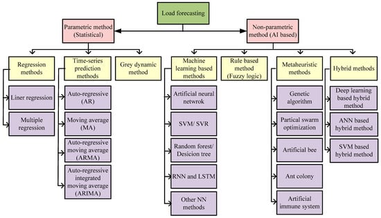
Figure 4.
Different methods used for load forecasting.
6.1. Parametric Method
A parametric method is a linear model whose data are analyzed considering the collected parameters. The number of parameters used are of fixed size and independent of the number of training cases. This method first selects the function form, and then uses training data to learn function coefficients. This consists of a mathematical relationship between a random variable and another non-random variable [50]. For load forecasting, a parametric model can be classified into different types, which are as follows.
6.1.1. Regression Method
The regression method is a statistical method which is used to forecast the future values of a variable using other variables. It can also be stated that it is a technique used to determine the relationship between dependent variables and one or more independent variables [51]. The objective of the regression method is to provide a function which is very close to the relationship between the variables, which, in result, predicts the values of the dependent variables using independent variables [51]. It is bifurcated into two methods: linear regression and multiple regression. If there is a relation between two variables, then it is known as simple linear regression, and if there is a relation between more than two variables, then it is called multi-variable linear regression [52].
Linear Regression
Linear regression is a method which is used to find the relation between two variables. As the relationship between two variables is found, the parameters have to vary with the same relation. Furthermore, the same relation is applied to the predicted parameters. This provides the values of dependent variables in terms of independent variables [52]. Borges et al. [53] proposed a method for STLF in three different categories: (a) a top-down method: summing up single consumptions and then executing global forecast, (b) a bottom-up method: adding the sum of load forecasts on single consumption, and (c) a regression method: forecasting is based on the regression of each load measured by the smart meter. The MAPE obtained by the proposed methods were 6.28% and 7.22%.
Fan et al. [54] presented an STLF model using semi-parametric additive models. This model is a statistical model which determines the relationship between load demand and driver variables. The variables considered here are: forecasted temperature, calendar variables, lagged actual demand, and historical load data of a particular region in the power system. Additionally, a modified bootstrap method is used to determine prediction intervals. This method is used to predict the load in half-hourly demand up to seven days ahead for the defined region. Here, the test case of the Australian National Electricity Market was considered. The performance of the proposed method was evaluated by calculating the MAPE, which was 1.88%
Multiple Linear Regression
In this method, dependent variables are related to two or more independent variables. In addition, the load is determined in terms of independent variables like weather and other factors which directly affect the electrical load [51,55]. Hong et al. [55] presented a practical approach for the LTLF using multiple linear regression models working on an hourly data basis. In this study, the LTLF was bisected into three components: predictive modeling, scenario analysis, and weather normalization.
6.1.2. Time Series Prediction Method
The time series prediction models are categorized into moving average, autoregressive, autoregressive moving average, and autoregressive integrated moving average models. In the autoregressive model (AR), forecasting is performed using previous data in which there is a linear regression relationship between the current data and the previous data. In the moving average (MA) model, the forecasting is performed from the white noise of previous data, where there is no linear regression relationship between current data and previous noise data. In the ARMA model, first, the AR parameters are estimated, and then MA is estimated based on the obtained AR parameters. The ARMA model was first introduced in 1970 by Box and Jenkins [55,56,57]. In addition, they also introduced an autoregressive integrated moving average (ARIMA) model that is like the ARMA model. In ARMA, the predicted value of time series has a linear relationship with the past historical values and lags of white noise [58]. Since AR, MA, and ARMA models are used for stationary time series data, they are not adequate for non-stationary time series data. Hence, the ARIMA model was introduced [57,59]. Here, AR obtained from the regression of the variable of its own lagged (previous) value is combined with MA obtained from the linear combination of several residual (or error) terms at various times in past [60]. The word ‘integrated’ in ARIMA signifies that the number of differences are already applied to make the model stationary. In the mathematical representation, the order of AR is denoted as ‘p’, the order of MA is denoted as ‘q’, ARMA is known as ‘p, q’, and the order of ARIMA is denoted as ‘p, d, q’, where d is the degree of differencing. The mathematical expressions used for AR, MA, and ARMA are shown below [60].
Autoregressive (AR) Model
In the case of autoregressive models, forecasting is based on the linear relationship between current data and previous data. The formula for the AR model is expressed as shown in Equations (10) and (11).
where is the time series data, is constant, … are model parameters, and is random variable white noise. In terms of lag operator (T), AR (p) is given by Equation (12).
Moving Average (MA) Model
The formulas for the moving average model are given in Equations (13) and (14).
where is the expectation of , … are model parameters. In terms of lag operator (T), MA (q) is given by Equation (15).
ARMA Model
The ARMA model is combination of the AR and MA models. In ARMA, forecasting is performed on the basis of the linear relationship between current data, previous data, and white noise. The formula used for the ARMA model is seen in Equation (16).
In terms of the lag operator, ARMA (p, q) is given by Equation (17).
ARIMA Model
The ARIMA (p, q, d) model is similar to the ARMA model and can be expressed as seen in Equations (18) and (19). Here, d is the degree of differencing.
Newsham et al. [61] introduced a STLF model using the ARIMA method for hourly forecasting. In their study, the authors used occupancy data on building level. The data were collected using various sensors installed in the building. The MAPE was calculated for both the occupancy and without the occupancy period, and was recorded as 1.217% and 1.244%, respectively.
Wang et al. [58] introduced a hybrid model for load forecasting by integrating the ARIMA and ANN methods together. While ARIMA can work with linear relationships of present and past values, and cannot deal with non-linear relationships, similarly, ANN alone cannot deal with both linear and non-linear relations of present and past values equally. Hence, a hybrid model was proposed that exploits both ARIMA and ANN characteristics equally. For an experimental purpose, the consumption data of the Hebei region from China were taken under consideration from 2009 to 2013. The performance was evaluated by three measures: RMSE, MAE, and MAPE, whose values were 92.45, 73.8, and 0.311%.
Chujai et al. [62] proposed a time series electrical forecasting method considering a household load using the ARIMA and ARMA models. In the forecasting process, daily, weekly, monthly, and quarterly time horizons were taken into consideration. For the evaluation, the RMSE of both models were determined. Here, the dataset of an individual user’s consumption was taken from Dec. 2006 to Nov. 2010 for the experimental evaluation. After the modeling of both the models, it was presented that ARIMA was favorable for the time horizons of monthly and quarterly forecasting, whereas ARMA was most suitable for daily and weekly forecasting.
Almeshaiei et al. [63] proposed a pragmatic methodology for electric load forecasting. The presented methodology is based on the principle of load pattern decomposition and segmentation. Here, the moving average (MA) method was considered for the load pattern decomposition. In this article, the proposed methodology was explained in five steps: primal visual and descriptive statistical analysis, contour formation, load pattern decomposition, segmentation, and future load forecasting. For the analysis purpose, the daily energy consumption of the Kuwaiti electric network was taken from 2006 to 2008. The model was then evaluated by MAPE and resulted in the value of 0.0384%.
Zhang et al. [64] demonstrated a hybrid short-term load forecasting model using improved empirical mode decomposition (IEMD), ARIMA, and wavelet neural network (WNN), optimized by a fruit fly optimization algorithm (FOA). IEMD is applicable for non-linear and non-stationary series and is used for reducing the loss of information. The ARIMA model fits well with the linear component of the original load. WNN optimized by FOA can fit the non-linear component of the original load. By hybridizing and adopting the advantages from each model, an accurate forecasting was achieved. For modeling, a dataset of electrical load data from Australia and New York were used.
6.1.3. Gray Method
In commercial terms, gray is a mixture of white and black. In technical terms, gray represents the combination of known and unknown values. The gray model was extracted from the gray relational analysis (GRA). It was firstly developed by Deng Julong in 1982 [65]. Gray systems are those in which some data or information is known and some is unknown. They work on uncertainty, where uncertainty is defined in terms of incomplete and inaccurate information [66]. In most cases, a gray model (GM) with a first-order differential equation and one variable denoted as GM (1, 1) is widely used for load forecasting process [67].
Tang et al. [67] proposed a GM based on a genetic algorithm. Here, the genetic algorithm optimizes the starting value and background value of a differential equation. A gray model with back propagation (GBP) neural network model was proposed in addition to the GM, which was then compared with the GM and found to perform better than the GM in terms of stability and decision-making. The maximum relative percentage error was obtained in the year 2009, which was 3.2%.
Hsu et al. [68] presented an improved gray model for load forecasting. In this model, the residual modification of the GM is done with an artificial neural network sign estimator. The model was studied on the electricity power consumption in Taiwan. The MAPE of the GM(1,1), ARIMA, and improved GM(1,1) were calculated as 3.88%, 2.2%, and 1.29%.
Lee et al. [69] proposed a load forecasting scheme integrating a gray model with genetic programming. For providing the accuracy of forecasting, genetic programming (GP) sign estimation was used. Additionally, GP does not depend upon any dependent or independent variables. For the analysis, Chinese energy consumption data from 1990 to 2007 were considered.
Hamzacebi et al. [70] proposed annual electricity forecasting using an optimized gray model (1, 1). The optimized gray model (1, 1) was used for both direct as well as iterative manners. The dataset of Turkey from 1945 to 2010 was collected and electric load forecasting was performed from 2013 to 2025. From the analysis, it was found that the direct forecasting was much better than iterative forecasting, with a MAPE of 3.28%.
Jin et al. [71] worked on STLF, using a hybrid optimized gray model (HOGM) based on multi-strategy contest and segmented gray correlation. This model merges internal with external optimization. The external factors are described as climatic (temperature and humidity) and social (weekdays and holidays) impact factors in load consumption. Although the GM (1, 1) model provides a better forecast of rising and falling power loads, it fails to predict loads during mutations. For the analysis purpose, a dataset (hourly data) from January 2009 to June 2009 was considered and the forecasting error of 4.91% was recorded with the HOGM method.
Bahrami et al. [72] proposed a new model for STLF by integrating a wavelet transform (WT) and a gray model. In this model, historical energy load data consumption and weather-related data are taken as input. WT is used to filter out the unwanted and irrelevant data. Training is done with the particle swarm optimization method, which determines the parameters of first-order GM (1, N) with N input. After this, the day-ahead load forecasting is modeled and the analysis of the result is performed by various measures like absolute percentage error, MAPE, MAE, mean percentage error, daily peak error, and weekly peak error.
Mi et al. [73] proposed a STLF using an improved exponential smoothing gray model. In this improved model, the smoothing of original load data is processed using an exponential smoothing method first. Then, a gray forecasting model with an optimized value is built using the smoothed sequence data. At last, the forecasted value is restored with an inverse exponential smoothing method. The efficiency of the stated method is measured by knowing the value of the MAPE. The average MAPE of the proposed model was found to be 1.26%.
6.2. Non-Parametric Methods (Artificial Intelligence-Based)
The non-parametric methods are also known as artificial intelligence (AI)-based methods. With these methods, the number of parameters does not need to be fixed, but can vary with the sample size. Statistical methods are not suitable for non-linear input variables, can be limited to only a few solutions, and may take a long time to compute [44,74]. Additionally, a large error is found in parametric approaches when there exist environmental changes, such as changes in weather and different types of days (normal day, holiday, or festival day) [44]. In order to overcome this disadvantage, non-parametric or artificial intelligence models are proposed. The number of parameters in this method depends on the amount of training data. A description of the different types of non-parametric models is found below.
6.2.1. Machine Learning (ML)-Based Methods
In order to overcome the difficulties faced by hard-coded knowledge systems, AI techniques must be able to learn from the raw data by extracting patterns. This capability is termed machine learning [45]. A neural network is a subset of machine learning. It is structured from the nervous system of the human body, in which the network of neurons bonded biologically is known as the biological neural network. Today, artificial neural networks are being used that are composed of artificial neurons. In humans, brains are made up of many connected neurons. Similarly, in a neural network, the network is formed by connected nodes. In [45], there is a discussion about how learning happens in biological brains in the earliest algorithms, and perhaps this is why ANNs are named that way. In neural networks, neurons are connected by connecting weights, as shown in Figure 5.
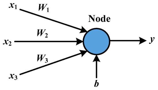
Figure 5.
Structure of a node showing inputs and output.
In the above figure, x1, x2, and x3 are the inputs to a node whose weights are assigned as W1, W2, and W3. b is the bias, which is directly related to the storage of information, and y is the output.
According to the architectural view, an NN contains three layers: input layer, hidden layer, and output layer. An artificial neural network (ANN) has the same structure as neural networks, as shown in Figure 6. Upon receiving a defined input, neurons generate their output according to their activation function, where the activation function is determined by weighting and input parameters [74,75,76]. The NN with single hidden layer is classified as an ANN. However, the NN with two or more hidden layers is classified as a deep neural network (DNN) [77,78]. The DNN is also an engineered system which is inspired by the biological brain [45]. For both ANN and DNN, the structure is shown in Figure 6a,b [75,76,77,78].
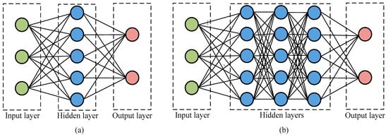
Figure 6.
Neural network categories: (a) ANN with a single hidden layer, (b) DNN with multiple hidden layers.
ANN provides the capability for AI to solve various problems. An ANN is used to perform image analysis, speech recognition, and adaptive control in artificial intelligence [45]. In the early 1980s, Hopfield [79] introduced a neural network with feedback, which acts as an associative memory. In order to enhance the technology, Rumelhart et al. [80] proposed new training methodologies called back propagation training and feedforward networks, which are based on inputs and outputs from a training set.
Artificial Neural Network (ANN)
Azadeh et al. [74] presented an article based on artificial neural networks (ANNs) for predicting power consumption over the short-term in heavy industrial loads. Furthermore, they also estimated an annual consumption using an ANN-based multilayer perceptron (MLP) technique with reduced error. In this article, the best network was selected using mean absolute percentage error and then compared with test data. The model was finally compared with actual data for validation and also compared with a conventional regression model through analysis of variance. The MAPE of the MLP method was calculated as 0.0099%.
Javed et al. [81] proposed an ANN- and SVM-based STLF model for multiple loads, also known as short-term multiple load forecasting (STMLF) in smart grid. In this scheme, they showed the use of anthropologic and structural data within STMLF. The combination of ANN and SVM increases the efficiency of forecasting for both AI- and statistical-based load forecasting. The result showed that the mean square error, on average, was 2.73 kWh, with a maximum of 3.42 kWh.
Webberley et al. [82] studied an ANN-based STLF method. This work considered a three-layer feedforward network as the ANN for study. An ANN model was applied here with temperature, hour of day, and day of week codes as inputs, and predicted load was the output. The accuracy of the presented method was determined by the mean absolute percentage error (MAPE). The lower the MAPE, the more accurate the prediction model.
In [11], a review on various ANN-based models for STLF was presented. A novel approach to training radial bias function in machine learning was studied and compared with earlier techniques. Here, larger datasets were used to train radial basis function (RBF) using decay RBF neural networks (DRNN), support vector regression (SVR), extreme learning machine (ELM), improved second-order algorithm (ISO), and error correction algorithm (ErrCor). These algorithms were compared on the basis of MAPE, and it was found that SVR and ELM showed a better result among the others. The MAPE value obtained was less than 2%.
Alobaidi et al. [43] proposed an ensemble learning model called ensemble artificial neural network (EANN) for day-ahead load forecasting on a household level. The proposed method offers a two-stage resampling plan. During the first stage, the entire dataset is divided into various sizes (or sub-models) of the ensemble model, often referred to as the re-sampler. Afterwards, in the second stage, random resamples are created and accurate information is exchanged between all samples collected during the first stage. For the training purpose, the ensemble diversity investigation was used in this method. The diversity was formed by the very first ensemble learning component. In this article, the EANN model was compared with a single ANN model and an ANN-based bagging model (BANN).
Support Vector Machines/Support Vector Regression
SVM is a supervised learning approach which was developed by Cortes and Vapnik in 1995 [26,45]. SVM is generally used for classification and regression analysis [44]. In the past few years, SVM has been widely used for regression analysis, pattern recognition, time series prediction, and load forecasting purposes [50]. SVR is used to train the SVM for estimating a function, which is then used to execute many machine learning tasks, including regression analysis and time series prediction [26]. The SVM algorithm creates a decision boundary which distributes various dimension spaces into classes. The decision boundary is called hyperplane. SVM selects the extreme values/vectors for the formation of hyperplane, and these extreme vectors are called support vectors. SVM has a kernel function/trick which converts low-dimension input space into high-dimension space. The kernel function can be written as the dot product between the input vectors [45].
Hong et al. [83] proposed a support vector regression with immune algorithm (SVRIA)-based load forecasting model. The model was carried out by taking the dataset of the Taiwan regional electric load from the year 1981 to 2000. In order to facilitate training, validation, and testing, the respective data for 1981 to 1992, 1993 to 1996, and 1997 to 2000 were separated. A comparison of the SVRIA model with SVRG, ANN, and regression models was presented in this article; the SVRIA model was found to be superior to others for better load forecasting.
Elattar et al. [84] proposed a new method for load forecasting by combining support vector regression (SVR) and locally weighted regression (LWR). Furthermore, the Mahalanobis distance was used to provide a weighted distance algorithm to optimize the weighting function bandwidth for the better accuracy of the algorithm. Based on the comparison with LWR, local SVR, and some other methods published earlier for the same datasets, it is clear that the proposed method is superior in predicting the load than other methods. In the proposed method, the phase space of time series was reconstructed using embedding dimension and delay constant. Euclidian distance was then used to determine the neighboring points of each query point. In order to calculate the new regularization parameter of SVR, each point in the neighborhood was weighed according to its distance from the query point. Finally, these neighboring points were used to train the model for load prediction, instead of using all the data.
Ghelardoni et al. [85] presented an LTLF method that predicts time series energy consumption data for one year on a half-hourly basis. The proposed method explores the empirical mode decomposition (EMD) technique based on SVR for effective long-term forecasting. In the EMD method, the time series data are decomposed into various intrinsic mode functions (IMFs) and, based on the information, the desired IMF is taken for consideration. Principal-IMFs (P-IMF) are estimated using the support vector regression for the P-IMF (SVP) procedure, which describes the general trend of a series, whereas Behavioral-IMFs (B-IMF) are estimated using the support vector regression for the B-IMF (SVB) procedure, which provides information about local characteristics.
Ko et al. [86] presented a hybrid approach for STLF. The SVR, radial basis function neural network (RBFNN), and dual extended Kalman filter (DEKF) were combined together to form a prediction model (SVR-DEKF-RBFNN). Here, SVR is used to decide the initial parameters and structure of RBFNN. As part of the learning algorithm, DEKF is used, which also optimizes key parameters. The final step involves short-term load prediction using RBFNN. The MAPE of the proposed hybrid method for both 24 h- and 72 h-ahead forecasting were obtained as 0.56% and 0.33%.
Random Forest (RF) and Decision Tree (DT)
Random forest is a supervised learning technique in machine learning. It can be used for both classification and regression analysis in ML. RF contains a number of decision tress in various subsets of a given dataset, and computes the average to improve the forecasting accuracy of that dataset [87]. Figure 7 shows the working process of RF [87].
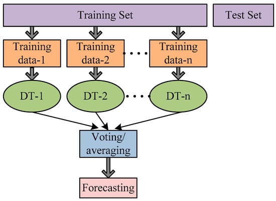
Figure 7.
Working process of random forest.
Decision tree is a machine learning algorithm which splits the input space into many regions and contains separate parameters for each region [45]. The structure of DT is shown in Figure 8 [45]. Each node of DT is part of a region in input space. The internal/decision nodes split that node into sub-regions. Hence, the entire space is sub-divided into non-overlapping regions. Here, in the figure, the circles denote internal/decision nodes and squares denote leaf nodes. The leaf nodes are associated with the outputs of the model.
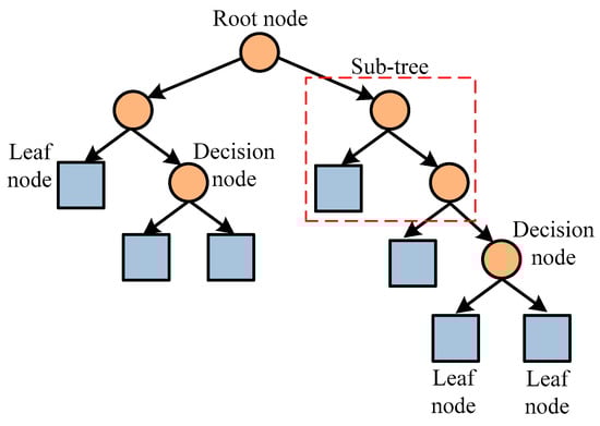
Figure 8.
Structure of decision tree.
Lahouar et al. [1] presented day-ahead load forecasting (basically STLF) using the random forest method with an expert input selection to refine the input. In this method, the demand for load consumption during the next 24 h is predicted. To overcome sudden variations in load, an online process is performed during the entire test period. An expert selection is used to handle complex load behavior and any special cases specific to high temperature, various religious events, moving holidays, etc.
Hsiao [23] presented a different approach to VSTLF for household loads. This forecasting is based on an individual’s load consumption based on context information (such as: local weather-, special events-, holiday-, day of week-, etc.-related data) and analysis of the consumer’s daily schedule. Here, two types of context information are taken under consideration: (a) day-dependent and (b) minute-dependent. In accordance with the different types of energy consumption behavior patterns, context features are classified into two groups; inter-cluster classification model and intra-cluster classification model. The day-dependent context features are classified in the inter-cluster classification model, whereas minute-dependent context features are classified in the intra-cluster classification model. In the proposed scheme, a decision tree classification is used for the inter-cluster model and a back propagation neural network is used for the intra-cluster model. Various methods were also considered for a comparative analysis, such as linear regression, SVR, SVR based on similar historical days (SVR2), random walk algorithm (RW), and the ARIMA model. The MAPE obtained were 3.23% and 2.44%.
Hambali et al. [27] proposed a novel method for load forecasting based on a decision tree (DT) algorithm. In DT, three methods are proposed; classification and regression trees (CART), reduced error pruning trees (REPTree), and decision stumps (DS). There are various evaluation indicators assigned to each method for the purpose of identifying the best method among the others. Based on the performance and evaluation, it was declared that the reduced error pruning tree method was better than the other two. In the proposed scheme, the data were first pre-processed to cover the missing data and reduce the imbalanced data, and then the data were used for training and testing purposes. The MAE and RMSE obtained were 0.0219, 0.0213, and 0.0615 and 0.1064, 0.105, and 0.1754.
Recurrent Neural Network and Long Short-Term Memory
The recurrent neural network (RNN) is a type of deep learning NN which is a subgroup of machine learning technique and is a main tool in handling sequential data with variable length of inputs or outputs [45]. In a neural network, the size of input and prediction output are fixed. However, it does not work with unknown size or sequential data. To overcome this limitation, an RNN is proposed. Though RNNs can also be used for fixed dimensions of input and output data, the important process is to properly manage the input data. It is also possible to use fully connected NNs for sequential data, but their main limitation is that they are unable to exploit the sequential structure of the data [45]. Therefore, RNN is widely used for handling sequential data (or unknown input size) with variable length of inputs or outputs. This can be achieved through the process of parameter sharing in the model, using datasets of different lengths, which further generalizes the sequence lengths during the training. In an RNN, the weights of artificial neurons are shared across various instances, and the same weights are re-used at each time step, allowing the network to use the sequential input of different lengths [45]. During the learning process, the RNN stores the previous output results in internal memory and then employs them as input again, as shown in Figure 9a [45,88,89]. In an RNN, recurrent means performing identical functions at each time and relating the result to previous calculations [88]. The unfolding network structure of an RNN is shown in Figure 9b [45,88,89]. Here U, V, and W are the weight matrices for three types of connections: input to hidden, hidden to output, and hidden to hidden, whereas the state of the system is represented by s [45].
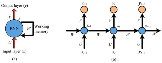
Figure 9.
Structure of recurrent neural network: (a) Single line structure of RNN, (b) Unfolding network of RNN.
RNN has many advantages, such as: it can memorize by storing previous results, it can be used to process sequential data, it can work for any input size, and it considers current and previous data for calculating new results. Apart from many advantages, RNN has several disadvantages, such as (a) its tanh and sigmoid activation functions are not capable of processing long sequence information because of a large input gap [89], (b) due to recurrence in nature, it takes more time, (c) exploding gradient, (d) vanishing gradient, and (e) complications in training the data.
Therefore, to overcome the above disadvantages of RNN, long short-term memory (LSTM) was developed by Hochreiter and Schmidhuber in 1997 [89]. In LSTM, introducing gate functions may help in handling long-term information. As a result, a forget gate is introduced in addition to an input gate and output gate [90]. Furthermore, this eliminates the possibility of vanishing gradient and exploding gradient. In addition, data can be trained quickly. Earlier RNNs consist of a single hidden state, which is adequate for short-term input. However, LSTM was constructed with two hidden states to capture both short-term and long-term inputs [91]. The flow process and internal structure of LSTM are shown in Figure 10a,b [88,89,90,91].
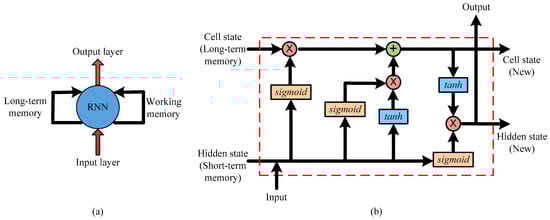
Figure 10.
Structure of LSTM network (a) Flow process of LSTM, (b) Internal structure of an LSTM.
The LSTM network has LSTM cells with an internal recurrence (self-loop) in addition to the outer recurrence of RNNs. It consists of the same inputs and outputs as a normal RNN, but has more parameters and the presence of gating units to control the information flow [45].
Fan et al. [92] worked on building energy predictions by using various strategies based on recurrent neural networks. The characteristics of these strategies are further categorized into high- and low-level. In high-level, three different approaches are presented for the forecasting of short-term load information, namely recursive approach, direct approach, and multi-input and multi-output approach. Similarly for low-level, state-of-art methods using 1-D convolutional process, bidirectional process, and different types of recurrent units are defined.
Marino et al. [93] proposed a deep learning neural network (DLNN)-based STLF by taking one-minute and one-hour resolution data. In this proposed scheme, the LSTM deep learning approach is used. The LSTM technique is used in two architectures; standard LSTM and sequence to sequence-based LSTM (S2S). Based on simulations of both the architectures, it was observed that standard LSTM does not predict well for one-minute resolution, but it predicts is suitably for one-hour resolution. However, after simulating the second method, it was clear that S2S architecture provides a good load forecasting for both one-minute and one-hour resolution. The RMSE obtained for both resolutions of training and testing data were 0.701, 0.625 and 0.742, 0.667.
Bouktif et al. [94] presented a hybrid method for load forecasting using both multi-sequence LSTM-RNN and a metaheuristics technique. In many instances, LSTM alone is unable to predict future load consumption due to the presence of noise in the dataset, as well as a naive selection of hyperparameters. To overcome this, metaheuristic algorithms were proposed that optimize LSTM hyperparameters. Hence, they proposed a genetic algorithm (GA) and particle swarm optimization (PSO) model for efficient load forecasting. They collected half-hourly electricity consumption data from France for nine years, starting from 2008 to 2016.
Jin et al. [95] proposed a new technique for STLF to strengthen the forecasting technique. They proposed an integrated approach by combining variation mode decomposition (VMD), LSTM, and a binary encoding genetic optimization algorithm for predicting the best outcome. In this scheme, first, the original load series data are decomposed to various components and reconstructed to eliminate the noise from original data so as to extract the features from the decomposed data. LSTM technique is applied to obtain forecasted power. Here, a binary encoding genetic algorithm is used to confirm the hidden layers and input data for LSTM. It was noted that the minimum MAPE values of the proposed scheme were 0.3717%, 0.3486%, and 0.9800%.
Rafi et al. [96] proposed an integrated method for STLF using a convolutional neural network and LSTM. The historical power consumption data from the Bangladesh Power System from January 2014 to December 2019 was used, from which five-year datasets were taken for training purposes (from 2014 to 2018) and the last year’s data were considered for evaluation purposes. A comparative analysis of the CNN-LSTM method was done with other methods such as LSTM, RBFN, and XGBoost. Based on the various measures like MAE, RMSE, MAPE, and R-square, all methods were compared.
Other NN-Based Methods
Amarasinghe et al. [97] proposed a deep NN-based STLF model using a convolutional neural network (CNN). A historical dataset obtained by one customer was used to test the method. The data were collected from the year 2006 to 2010 with one-minute resolution. In the proposed scheme, the testing was performed with CNN, with different convolutional layers, and it was observed that the performance did not vary much in different architectures. To justify the best use of the suggested method, it was compared with other methods such as ANN, SVM, LSTMs, and factored restricted Boltzmann machines (FCRBM). The obtained results were best among all stated methods for accurate forecasting. The best value of RMSE obtained was 0.732.
Gao et al. [98] provided an interesting model for STLF based on EMD, gated recurrent unit (GRU), and feature selection (FS) methods. In this method, actual load series data are decomposed into various sub-series using the EMD technique. Then, the Pearson correlation coefficient method is used for analyzing the relationship between sub-series and actual load series data. The highly correlated sub-series with actual load series are considered features in the input of GRU to establish a prediction model. The developed model was compared with GRU, SVR, and random forest (RF) models, and also compared with hybrid models EMD-GRU, EMD-SVR, and EMD-RF. The results showed that the integrated FS-EMD-GRU method is more accurate than all other NN-based methods.
6.2.2. Rule-Based Method (Fuzzy Logic-Based)
A fuzzy set was introduced by Zadeh for the first time in 1965. The fuzzy logic method is rule-based and easy to implement when compared to conventional methods [99]. A fuzzy logic approach is also suitable for forecasting load considering uncertainties such as temperature variations, humidity, seasonal effects, weekdays and weekend days, and festivals. Therefore, this approach is very suitable while considering the non-linear relationships between various factors [100,101]. The operation of fuzzy logic-based forecasting is shown in Figure 11 [102].
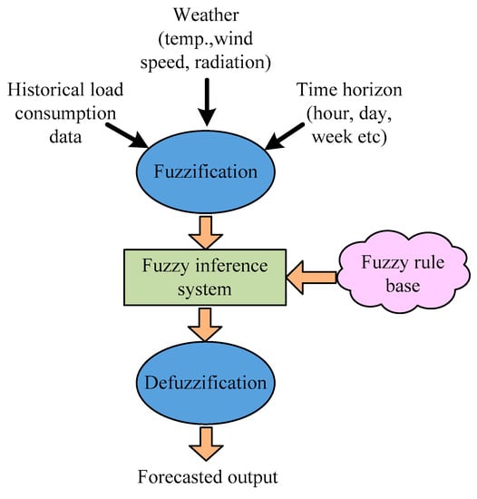
Figure 11.
Fuzzy logic-based load forecasting.
In the figure, historical load consumption data, weather-related data, and time horizons are inputs for the fuzzification. In the fuzzification stage, the crisp set is converted to a fuzzier set [103]. After fuzzification, these data are then transferred to fuzzy inference. By utilizing fuzzy rules that the forecaster prepares, the inference system executes the task of forecasting. Additionally, forecasting accuracy depends on the rules outlined by the forecaster. Finally, the fuzzified output is converted to crisp output in the defuzzification process [102].
Yang et al. [104] presented a scheme combining NN and fuzzy logic methods for load forecasting. Historical consumption data were used for neural networks, whereas weather conditions and holidays were considered for fuzzy logic interference. The integration was done only for forecasting short-term loads.
Ali et al. [101] proposed a fuzzy logic-based LTLF model for year-ahead forecasting. The fuzzy logic model was formed by considering the historical load consumption data of one year and weather-related data such as temperature and humidity. The analysis of model was done in the town of Mubi in Adamawa state and observed a MAPE of 6.9% with 93.1% efficiency.
Ali et al. [102] proposed STLF using fuzzy logic. For this method, a previous day of similar load, time, and temperature are taken as variable parameters. Each of these parameters is then processed with the Mamdani rule to obtain the forecasted output. The proposed method was compared with conventional method and found an error in between +12.14% and −9.48%.
Černe et al. [105] presented an STLF for day-ahead forecasting using an adaptive fuzzy model (Takagi–Sugeno model). Here, the load forecasting problem is divided into three sub-problems: average daily load, shape of load, and amplitude of load. All three problems are solved using the Takagi–Sugeno method. For analysis, data were taken from the southwest region of Slovenia for three years, from 2010 to 2012, in three sets. These sets included electrical load, weather-related data (temperature, humidity, wind speed, and solar radiation), and time-related data (hour, day, month, etc.). The reported model showed accuracy with a MAPE of 0.13%.
Faysal et al. [103] proposed STLF using a fuzzy system. Various parameters like temperature, humidity, season of year, and time segments of day are considered for determining electrical load demand. Each of the parameters is analyzed using the Mamdani and if–then rules. In this work, the energy consumption data were taken from the Bangladesh Power Development Board (BPDB) for one year, from 2017 to 2018.
Jain et al. [106] proposed a method for STLF using fuzzy logic and the swarm intelligence technique. Here, the average of load consumed, temperature, and humidity is used as input for the model. Particle Swarm Optimization (PSO) and Evolutionary Particle Swarm Optimization (EPSO) techniques were used on the training dataset for the tuning of fuzzy input parameters. Using data from previous historical forecast days and similar days, the correction factor was estimated by both techniques for the selected similar day to the forecast day. The model was studied in MATLAB using data from 3 years, from November 1996 to November 1999. The result showed that the value of MAPE was below 3%.
In addition to the above discussed research, fuzzy logic systems have also been implemented in other studies [107,108,109,110,111].
With the successful implementation of the fuzzy logic-based method, the adaptive neuro-fuzzy inference system (ANFIS) has now been implemented to facilitate learning capability [112,113]. In this new method, a hybrid learning rule is proposed which integrates the gradient method and least square estimate for the parameter identification. ANFIS works in five different layers, as shown in Figure 12 [113].
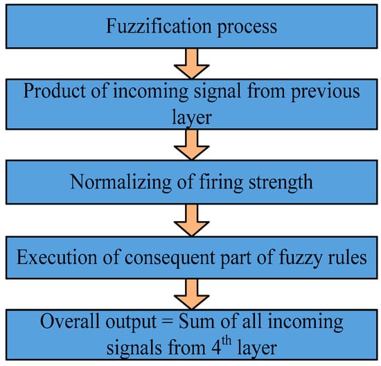
Figure 12.
Layers of adaptive neuro-fuzzy inference system.
Laouafi et al. [113] studied the adaptive neuro-fuzzy inference approach for the daily and weekly load forecasting. In this method, the seasonal effects of daily and weekly cycles are used to determine consumption pattern of electricity. The electricity load consumption in France was presented for the assessment of the method reported in [113]. In this study, half-hourly consumption data were considered from 01 January 2014 to 27 June 2014. The result showed that the MAPE in the ANFIS model was 2.087%.
Akarslan et al. [114] also worked on an adaptive neuro-fuzzy inference approach for load forecasting in smart grid. In this method, only hourly load consumption data is collected and then the first-order derivative of load consumption, actual month, and actual hour data are used as the input of the ANFIS model. For the data collection, load consumption in the Cay vocational high school campus area of Afyon Kocatepe University was used from 1 April 2016 to 27 December 2017, where one year’s data, starting from 1 April 2016 to 1 April 2017, was used for training purposes and the remaining data were used for testing purposes. The RMSE value of the proposed method was 28.40%.
Ali et al. [115] proposed a novel hybrid load forecasting technique considering the weighted least squares state estimation (WLS), NN, and ANFIS techniques and termed it WLANFIS. The NN alone is unsuitable for power system state estimation, and WLS cannot determine non-linearity in power requirement; hence, the integration of NN, WLS, and ANFIS is used. NN helps in estimating the non-linearity in demand and WLS helps in estimating the state of the power system. For the validation of the integrated model, a Canadian residential dataset was considered from the years 2012 to 2014. The model was applied to IEEE 14- and 30-bus systems for the state estimation. The MAPE of this model was observed as 2.66%.
6.2.3. Metaheuristic Methods
The metaheuristic methods are optimization algorithms which are used to tune and optimize the parameters of learning models. With the help of metaheuristic models, the accuracy of any model increases by reducing the percentage error. In this section, various metaheuristic methods are described.
Genetic Algorithm (GA)
Genetic is a biological term that was introduced by Charles Darwin and is evolved from his theory of natural evolution. In his theory, the process of natural selection is discussed, where survival of the fittest individual exists and these individuals are then selected for reproduction to produce next generation offspring. Offspring’s characteristics are influenced by their parents. In engineering, GA can be used to generate the best optimal solutions for various optimization and search problems [116]. The function of GA is same as that of artificial intelligence and has six phases, as shown in Figure 13.
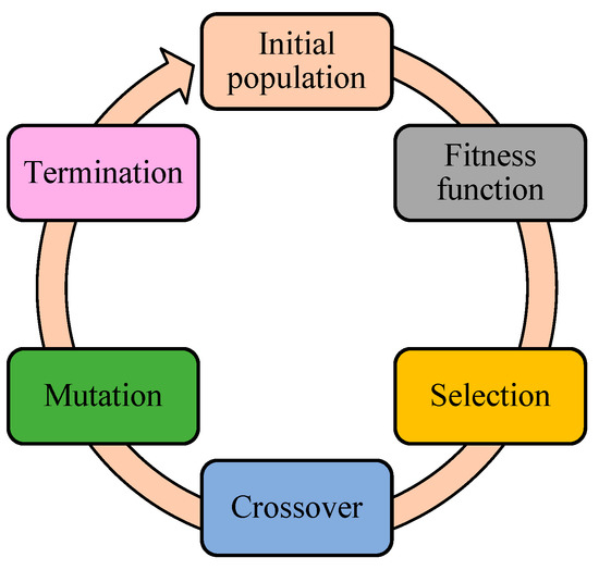
Figure 13.
Different phases of genetic algorithm.
Ling et al. [117] proposed a new model based on neural network (NN). The parameters of the new NN model were optimized using a genetic algorithm. The GA was applied with arithmetic crossover and non-uniform mutation. The forecasting error obtained was 0.0238 with a regression accuracy of 96%.
Gupta et al. [118] proposed a GA-based back propagation network (GA-BPN) for STLF. To obtain accuracy in load prediction, GA-BPN was used to determine the best suitable weight matrices for BPN.
Islam et al. [119] presented the utilization of a genetic algorithm for the optimization of a neural network for load forecasting. Before proceeding to the ANN structure, some set of parameters need to be defined. These parameters are categorized into two sets. In the first set, activation function, number of epochs, weights, and threshold are defined. In second set, the GA-related parameters such as population size, number of generations, crossovers, and mutations are considered. After setting these parameters, the ANN is trained. The performance of the technique mentioned in [96] was evaluated by calculating the MAPE, which was 5.85%.
Kalakova et al. [120] proposed a novel genetic algorithm (nGA)-based STLF. A multilayer ANN (MANN) is used to implement the forecasting model. nGA provides a solution for the dynamic economical dispatch problem in the power transmission network combined with STLF. The study of the proposed model was done on IEEE 9-bus and 30-bus system.
The genetic algorithm approach is also combined with some other methods to optimize parameters and improve load forecasting accuracy. Some of the combinations are recurrent support vector machines with GA [121], neural network and genetic algorithm [122], LSTM and GA [123], GA with SVR [124], etc.
Particle Swarm Optimization (PSO)
The idea of PSO was firstly presented by Kennedy and Eberhart in 1995 [125]. PSO is related to bird flocking or fishing schooling and swarm theory. The PSO method involves placing particles on an object in search space that correspond to any solution and having each particle assess the objective function at the point where it is. Each particle has a velocity associated with it. The velocities of the particles are dynamically adjusted according to their historical behavior as they traverse the search space. Consequently, particles tend to fly towards better and better search areas over time [126]. Thus, the fitness function of the entire swarm is likely to be close to optimum.
AlRashidi et al. [127] presented a PSO-based application for long-term load forecasting. Here, authors presented a new method of forecasting the annual peak load in electrical power systems. Forecasting is viewed as a problem for PSO and is shown in state space form. The parameters of different load forecasting models are determined by this technique. For validating the proposed technique, a dataset of Egypt and Kuwait networks was considered.
Wang et al. [128] presented a hybrid adaptive PSO model for load forecasting. This combined model is formed by the linear integration of time series models, such as seasonal ARIMA, seasonal exponential smoothing, and weighted SVM models. The weight coefficient of each individual model is then calculated by using adaptive PSO method. A comparison of each model was done with the combined model and found that the combined model is superior to the other models. The proposed method showed the mean accuracy of 30.746%, 45.358%, 45.494%, and 75.716%.
Xie et al. [129] proposed a STLF using a hybrid method combining an Elman neural network (ENN) and PSO. In this, the forecasting model is formed by using ENN, and the key parameter of ENN is set as constant. The learning rate of ENN is used as the key parameter for the model. The PSO is used to determine the appropriate learning rate of ENN. The method was compared with ENN, general regression neural network (GRNN), and back propagation neural network (BPNN). The RMSE values obtained were 0.1951, 0.2636, 0.4328, and 0.5445.
Qiang et al. [130] proposed a STLF using linear square-SVM (LS-SVM) and improved PSO. At first, the LS-SVM forecasted the load of the region of Taizhou, Zhejiang Province. Then, the improved PSO was used to optimize the parameters of the proposed SVM model. For checking the accuracy of the system, the MAE was calculated. The average and maximum MAE were obtained as 2.06% and 3.02%.
In [131], Ozerdem et al. proposed STLF using a feedforward neural network optimized by PSO. The training and network designing was done with a feedforward neural network and its parameters were optimized by PSO. For the comparison purpose, the PSO-optimized and back propagation-optimized feedforward neural network was trained. The training time, MAE, and mean square error (MSE) for both models were calculated. It was observed that back propagation neural network worked with less accuracy compared with the proposed model. In the data analysis, hourly load data provided by the Cyprus Turkish Electricity Authority (Kib-Tek) were considered.
Chafi et al. [132] proposed a STLF model based on NN and PSO. In this model, along with the improved PSO model, a three-layer feedforward NN trained by a back propagation algorithm is used to forecast the load. To test the STLF-NN-PSO, hourly load consumption data of Iran’s power grid was used from 22 March 2010 to 18 March 2013, from which the first 900 days’ data were used for training purposes and the remaining 193 days’ data were used for testing purposes.
Ren et al. [133] presented a load forecasting scheme based on particle swarm optimization with support vector machine (PSOSVM). The technique was proposed for long-term forecasting to predict annual power load. In this model, the structure and values of parameters are defined using a support vector machine. After this, the parameters are optimized using the PSO method. For study purposes, the annual electricity consumption dataset was selected from Beijing city from 1978 to 2010, from which the data from 1978 to 1997 were considered for training, and the remaining data were considered for testing purposes. The RMSE for the method reported in [133] was calculated as 2.53%.
Artificial Bee Colony (ABC)
The ABC is a swarm-based method which was proposed by Karaboga in 2005 [134]. Just like PSO, ABC is also motivated by the honeybee colony and its foraging behavior. An ABC model has three components: employed foraging bees, unemployed foraging bees, and food source. The first two components are directly related to the third component, i.e., employed and unemployed foraging bees search for rich and healthy food sources. Now, in terms of artificial intelligence, the foraging behavior of honeybees is synonymous with finding a better solution to any problem by optimizing the parameters.
Hong [135] presented an integrated model of load forecasting using seasonal recurrent support vector regression with chaotic ABC algorithm (SRSVRCABC). The SVR model is used to design seasonal electric load forecasting. RNN is used to figure out detailed information from the past data to feed to the SVR model. Then, a chaotic ABC algorithm is used to optimize the training parameters, which are used by the SVR for improving the performance of forecasting. For experimentation, the monthly electricity load dataset of northeastern China was considered from December 2004 to April 2009, from which the period of December 2004 to July 2007 was used for training, August 2007 to September 2008 was used for validation, and October 2008 to April 2009 was used for testing the dataset. The MAPE obtained was 2.387%.
Awan et al. [136] proposed an integrated model for STLF based on an artificial bee colony algorithm and ANN. Here, ANN is used to model the technique for load forecasting. For ANNs, ABC is used as an alternative learning method for optimizing neuron connection weights. This leads to forecasting the load with better accuracy. For the experimentation, an hourly power load demand dataset of 10 years (2002 to 2012) from the Independent Electricity System Operator (IESO) of Ontario State was used. In this study, a comparison was made between the model and a PSO-based ANN and a GA-based ANN model, and it was found that the ABC-ANN model was more accurate, having an MAPE of 1.89%.
Baesmat et al. [137] proposed a STLF to improve the accuracy of load forecasting. Their research relies on ANN and ABC algorithms. Here, the load forecasting is modeled using ANN, considering historical data and weather-related data. The ABC is used to optimize the learning process of ANN. A three-year dataset from the Bushehr province in Iran was considered for experimental purposes, in which the dataset of years 2014 and 2015 was used for training, and the next year’s dataset was used for testing the model.
Cevik et al. [138] presented STLF using ANN and ABC algorithms. In this method, ANN is also used to model the forecasting scheme by optimizing the parameters using an ABC algorithm, which also optimizes the neuron connection weights of ANN. Historical load data and weather-related data, like temperature and seasons, are used as input for the ANN network. In this study, hourly load consumption data from Turkey was considered from 2009 to 2012 and the temperature data were taken from the Turkish State Meteorological Service. The data from 2009 to 2011 were used for training purposes and the last year’s (2012) data were considered for testing purposes.
Aoyang et al. [139] presented a STLF model based on a radial biased function neural network (RBF-NN) and ABC. The training model of STLF is made using RBF-NN, which is a multi-layered feedforward neural network. The RBF-NN is trained by an artificial bee colony algorithm. The MAPE of the proposed model were obtained as 2.15%, 4.66%, and 3.70%.
Ant Colony Optimization (ACO)
ACO method is a probabilistic method which works on the action of an ant colony and motivated by the foraging behavior of ants. The ants travel in single direction to mark a designated path which is then followed by other ants in the colony. In search of food, ants explore the nearby surrounding area to their nests randomly. When ants move, they release a chemical substance called pheromones on the ground. The pheromone depends on the quality of food found by an ant. This pheromone is easily smelled by other ants. While searching for good food, these ants release a good concentration of pheromones, thus making a path for others. As they find their food, the ants take it back to their nest by following the path where the pheromones were originally released [140]. In this way, the pheromone trails guide other ants to follow the same path to a food source and return to their nest again [141]. Thus, an indirect communication occurs between ants and pheromone which is known as stigmergy. Hence, the foraging behavior of ants is based on the inherent evaluation of a solution and follows the shortest path rather than a longer one [142]. The foraging behavior of ants is transformed into artificial form, such that an artificial ant seeks out a good solution to a known optimization problem.
Niu et al. [142] proposed an STLF using SVM based on an ACO model. SVM is used for a load forecasting model and ACO is used for feature selection. A database from the Inner Mongolia region was collected for training and testing purposes, from which the power load data from 1 May 2004 to 31 March 2006 were used for training purposes, while the power load data from 31 March 2006 to 28 May 2006 were considered for testing purposes. For the evaluation of ACO-SVM supported by the ACO method, RMSE was calculated, which shows the accuracy of the model. The highest error rate obtained in ACO-SVM was 2.81%.
Ghanbari et al. [143] presented a hybrid computational intelligence (CI) model by integrating ACO, GA, and fuzzy logic for efficient load forecasting. The steps of the proposed scheme are as follows: (a) modeling a genetic algorithm-based learning process for the considered database, (b) using fuzzy logic, generating candidate rules, (c) using ant colony optimization for learning the fuzzy rules, and (d) evaluating the knowledge base. The ACO-GA model was studied on the annual load forecasting of Iran and was compared with ANFIS to show the superiority of the model.
Li et al. [144] introduced an improved ant colony clustering (IACC) algorithm for short-term load forecasting. IACC is more favorable to temperature and weather compared to the ant colony optimization algorithm. It is also superior to the clustering of similar load curves and reduces the internal distance of clusters for better accuracy in forecasting.
Ghanbari et al. [145] proposed a hybrid model by combining cooperative ant colony optimization, genetic algorithm (COR-ACO-GA), and fuzzy logic for load forecasting. The GA is used to generate a database of refined and fuzzy expert systems. ACO is used to generate a rule base in the system automatically. The COR-ACO-GA method was compared with ANFIS and ANN methods. To check the accuracy of the model, the RMSE, MAE, and MAPE were calculated in order to study the proposed model, for which the historical energy consumption data in Iran was considered from 1971 to 2007, from which the data from 1971 to 2000 were used for training and those from 2001 to 2007 were used for testing purposes.
Jain et al. [146] introduced a new approach for the STLF using a fuzzy inference system (FIS) and ant colony optimization. The calculation for STLF is done by FIS and then parameters are further optimized by ACO. The inputs of the model are previous day load, maximum temperature, and mean humidity. The MAPE obtained through this approach was 2.1%.
Artificial Immune System (AIS)
An immune system is a biological procedure in living beings and plays a vital role in protecting us from diseases. It has two terminologies which are interrelated to each other; one is antigen and the other is antibody. The immune system produces antibodies which resolve antigen. There is excitation between these antibodies and the excitation is based on the concentration of antibodies. As the concentration increases, the excitation also increases, respectively [147]. In the artificial immune system, the problem to be solved is acknowledged by antigens, whereas the solution to a problem is known by the antibodies. Antibodies with the greatest attraction (affinity) are known as memory cells [148].
Yong et al. [147] proposed a STLF using an artificial immune network (AIN). In this method, an immune algorithm is used to design a back propagation neural network (BPNN), which together are termed artificial immune network (AIN). The MAPE obtained using the NN model was 2.52%, and using the AIN model was 2.038%.
In [148], STLF was presented using an improved artificial immune algorithm (DAIA). In this article, DAIA-BPNN was proposed based on DAIA. The training and learning process is done by a back propagation neural network (BPNN) and DAIA is used to optimize the weight and threshold of the BPNN. For the study of the model mentioned in [148], historical load consumption data from California was considered, from which the data from June 2009 to August 2009 were used for training and data from 1 September 2009 to 14 September 2009 were used for testing purposes. For evaluating the accuracy, relative error (RPE), MAPE, and RMSE were calculated. The results showed the obtained value of MAPE and RMSE to be 1.51%, 2.62%, and 3.59% and 1.59%, 2.82%, and 3.68%.
Mishra et al. [149] presented a model using a hybrid artificial immune system. An artificial neural network is employed for a non-linear load. The ANN is trained by hybridizing back propagation, GA, PSO, and AIS. For evaluation, MAPE was calculated for the method, which was obtained as 4.2036%.
Santra et al. [150] proposed a method based on an artificial immune network. The mean actual load of the last three days is used for day-ahead hourly forecasting using immune memory. In the training phase, the proposed model is trained to generate immune network (IN). Each IN contains clusters and each cluster has an antibody. In the testing phase, the mean actual load of the last three days generated an antigen. For evaluation of the model, MAPE was calculated as 0.94%.
6.2.4. Hybrid Methods
Load forecasting through single methods has several disadvantages, such as high errors, reduced computing efficiency, impact on operating speed, etc. As a result, researchers are now trying to improve accuracy by combining the different methods in order to reach a better forecast. A hybrid model is the combination of two or more different models [26]. Feature engineering and optimization techniques are combined together in the hybrid models [28].
Deep Learning-Based Hybrid Models
Qiu et al. [151] proposed a hybrid method for load forecasting using EMD and a deep learning model. At first, the load series data are decomposed into various intrinsic mode functions (IMFs) and one residue with the EMD technique. A deep belief network (DBN) is used to model each IMF and the residue. A training matrix for each IMF and residue is modeled for input to the DBN. Every DBN is trained, which results in a prediction for each IMF and residue. In the end, all the predicted outputs are summed up to generate the aggregated load demand output. The performance of the proposed hybrid model was analyzed with RMSE and MAPE. For consideration, the dataset of the state of New South Wales (NSW) in Australia during three years, 2009, 2010, and 2011 were collected, and the data from years 2009 and 2010 were used for training purposes, and those of year 2011 were used for testing purposes. The MAPE obtained was 3%.
Qiu et al. [152] again proposed a hybrid method using discrete wavelet transform (DWT), EMD, and a Random Vector Functional Link network (RVFL). EMD alone has the drawback of mode mixing problems, and DWT can transform time series signals to frequency components. Therefore, EMD-DWT can perform proper decomposition, solving the frequency mixing issue created by EMD. The RVFL network uses random weights and closed form least square estimated separately from BP for the better tuning of weights. The working procedure of the proposed model is same as that presented in above model [129]. Through the EMD-DWT technique, each time series signal is decomposed into various IMFs and residue. After this, the training matrix is constructed as the input of each RVFL network. Each RVFL network is trained to provide the prediction output. All the outputs are then combined to provide the aggregated output. The performance of the model was evaluated with RMSE and MAPE, which were obtained as 108 and 1.2%.
Chao et al. [153] proposed a novel methodology for load forecasting using a deep learning model in which the features of the historical consumption data are filtered through stacked denoising autoencoders (SDAs). After feature extraction, the day-ahead load forecasting is modeled using a support vector regression model. Aside from the load data, the deep learning model also incorporates weather data. For the experimentation of model, an electricity load consumption dataset (in a per hour basis) from California/Los Angeles/New York City/Florida for the duration of 15 July 2015 to 10 September 2016 was considered, from which the dataset from 5 August 2015 to 15 August 2016 was used for training and that from 16 August 2016 to 31 August 2016 was used for testing purposes. The model was compared with simple SVR and ANN models. For the evaluation of the proposed model, the MAPE was calculated and figured out for all four cities: 2.67%, 0.9552%, 1.7261%, and 3.7631%.
ANN-Based Hybrid Models
Yuan et al. [154] proposed an ANN-based load forecasting model for forecasting hourly electricity consumption for the building loads of three campus areas in the Sugimoto Campus of Osaka City University, Japan. In this work, the future load was predicted using feedforward ANN which was trained with Levenberg–Marquardt (LM) back propagation algorithms. For the evaluation of the accuracy of the proposed model, correlation coefficient (R-square) and RMSE were considered. Six parameters: hour of day, day of week, hourly dry-bulb temperature, hourly relative humidity, hourly global irradiance, and previous hourly electricity consumption were used as input to the ANN model. The R-square obtained was in the range of 0.9%.
Bouktif et al. [155] proposed a STLF and MTLF using a recurrent neural network and the LSTM method By using feature selection and a genetic algorithm, the predictor variables, optimal lag, and number of layers are defined. For the study, a half yearly reading of electricity energy consumption in France from January 2008 to December 2016 was considered, and for evaluation, RMSE and MAE were calculated.
He et al. [156] proposed a STLF method using ANN with a back propagation (BP) algorithm. Since BP can easily adopt the variables related to weather into the model and best relate the input and output, it was considered along with ANN in this work. In addition to this, a similar day was conceptualized to eliminate the consideration of holidays and other factors. In this way, historical data were filtered for training purposes, which can improve simulation speed and reduce training time. The mean square error obtained were 4.26% and 2.64%.
Hamid et al. [157] also projected towards load forecasting using ANN and an artificial immune system (AIS) algorithm. In this proposed method, an AIS algorithm is used to train the ANN model and testing is done on a historical dataset. A comparative analysis of the proposed algorithm with an ANN-driven BP algorithm was conducted and found that the ANN-AIS system was more compatible than the ANN-BP system. The MAPE obtained was less than 3%.
Wang et al. [158] described a new method for electrical load forecasting (ELF) by combining various techniques. The steps involved in this paper are decomposition and denoising of original data sequences to decompose and reconstruct various modes of original data. These were performed using the EMD technique so as to reduce the presence of noise. After this, ANN-based models (BPNN, Elman, GRNN, ELMnn, and LS-SVM) were used for the forecasting, using the reconstructed data. The weights of each ANN model were optimized by a multi-objective slap swarm algorithm (MSsa).
In addition, Table 2 below provides an overview of some of the ANN-based hybrid models.
Table 2.
ANN-based hybrid models.
SVM-Based Hybrid Models
Xu et al. [172] presented a hybrid model for load forecasting in a power grid with distribution generation. In this model, the SVM method is hybridized with an immune algorithm and fruit fly optimization algorithm (IA-FOA) for the optimization of parameters. For load forecasting, hourly load consumption data and weather-related information are gathered and train the integrated model combining neural network and polynomial regression models. A comparison of the method with other regression techniques and AI-based methods was conducted. The dataset of load consumption and weather data of northeast China from 1 June to 31 June 2013 was used, which contains 744 datasets. Out of 744 datasets, 648 were used for training and the remaining 96 were used for testing purposes. For evaluation, MAE and MAPE were calculated, which provided the accuracy of system. The relative error was found to be about 2%.
Li et al. [173] proposed a least squares-support vector machine (LSSVM) using a fruit fly optimization algorithm (FOA). FOA is used to automatically determine the parameters of LSSVM. For the experimental simulation, the annual electricity consumption dataset of China was considered between years 1978 to 2011. The performance of the model was evaluated by MAPE, MSE, and average absolute error (AAE) and found in the range of −3% to +3%.
Zeng et al. [174] proposed a new method for STLF using a generalized regression neural network (GRNN) and a least squares-support vector machine (LS-SVM) based on a harmony search algorithm (HS). GRNN is used to select the special factors (economic factors such as salary and power price, and non-economic factors such as temperature, humidity, holiday, and rainfall) which influence load forecasting. The HS algorithm is used to determine the hyperparameters of LS-SVM. For the study of the proposed model, the power load consumption of a certain area in China was considered.
Kavousi-Fard et al. [175] proposed a hybrid forecasting model integrating support vector regression (SVR) and a modified firefly algorithm (MFA) model for STLF. SVR has nonlinear mapping features, whereas MFA is used to set the parameters of SVR. For the experiment, load consumption data provided by the Fars Electrical Power Company, Iran were used. The consumption recorded between 21 March 2007 and 20 February 2010 was considered, from which the data from 21 March 2007 to 20 January 2010 were taken for training purposes and the remaining were taken for testing purposes.
Hafeez et al. [46] presented a hybrid model for load forecasting using feature engineering (FE) and an optimization algorithm. The modified firefly optimization algorithm (mFFO) with SVR is used as an optimization technique along with FE, naming the hybrid technique FE-SVR-mFFO. In this, FE is introduced for enhancing the features for better computational performance. The mFFO algorithm optimizes the parameters of SVR for a better forecasting result. For examining the performance of the model, the half-yearly load consumption data in states of Australia (New South Wales, Queensland, South Australia, Tasmania and Victoria) were considered.
Zhang et al. [176] proposed a novel model combining SVR and an improved adaptive GA (IAGA) for STLF. The SVR is used to develop a load forecasting model and IAGA is used to optimize the input features of the SVR model and SVR parameters. The experiment dataset was taken from the state grid Heilongjiang Electric Power Co., Ltd., China, of six years, containing load consumption and weather factors of each hour. For the training, the dataset from 1 January 2012 to 30 June 2013 was used, whereas for testing, the dataset from 1 July 2013 to 14 July 2013 was considered.
7. Challenges Related to Load Forecasting Based on Conventional Meter Information
In view of the increasing load demand of domestic, commercial, and industrial customers, it is necessary to keep track of the energy consumption by equipment at regular intervals in order to avoid the unnecessary operation of equipment. It is not unusual for equipment to be allowed to run ideally for several hours at a time. This contrasts with load forecasting, which may assist users in reducing their power consumption and saving electricity. However, conventional meters are incapable of providing complete information regarding the consumer’s electricity consumption and do not provide a good load forecast due to a variety of reasons. The challenges associated with conventional meter-based load forecasting are discussed below:
- It is not possible to obtain detailed information about electricity used at the end level from conventional meter data, which was available in the past. Due to this, short-term load forecasts may have a reduced level of accuracy [177].
- In the case of conventional meters, it is impossible to obtain high resolution past data. As a result, forecasting cannot be made with any degree of reliability [178].
- STLF in a true sense is not possible using conventional meter information because, based on the collected past data, STLF is conducted. However, such data may vary, which depends highly on the type of consumer, weather condition, season, availability of supply, and operating condition of the power system. In other words, the monthly consumption information of end consumers is not useful for hourly load prediction.
- When readings are taken in bulk, there is a possibility of human error, which may impact the accuracy of the forecasting model.
- Due to the lack of a communication interface in conventional meters, two-way communication between consumers and control centers is not possible.
- A conventional meter cannot be programmed to automatically switch devices or equipment based on predicted values. Traditionally, conventional meters are not capable of alerting users when their electricity consumption exceeds the limit. The result is a high electricity bill or sometimes a direct power outage [40].
- Since the data control center manually enters load consumption details, the privacy of data cannot be guaranteed. This may result in data being intentionally used for forecasting by some organizations when similar data already exist.
- A conventional meter does not have any memory for storing data. Consequently, data analysis and pre-processing cannot be carried out for forecasting loads [179].
8. Advantages of Smart Meter-Based Load Forecasting over Conventional Metering System
Under conventional metering techniques, there are several models for load forecasting that are convenient and easy to use. Even though it has shown a huge variety of predictions of future load, smart meter-based load forecasting is much more reliable, fast to learn, and shows higher accuracy than traditional meter-based load forecasting. A smart grid system using smart meters has the following advantages over a conventional grid:
- Smart metering collects historical data directly through a database or server using a communication interface [34], whereas conventional metering collects historical data manually if recorded previously.
- Smart meters work with real-time data.
- Taking readings on smart meters does not require a specific time period. The data can be captured directly at any given time, including seconds, minutes, hours, days, etc., or be taken from its memory later. However, there are predetermined time intervals between readings of load consumption in conventional meters, such as 15 min, 30 min, an hour, etc.
- In a smart metering system, forecasting is more volatile towards both linear and non-linear models. In conventional metering systems, some of the non-parametric models also contribute to load forecasting for non-linear datasets, but they are not reliable for all types of non-linear patterns due to the problems of irrelevant specification, overfitting, or underfitting [48].
- A smart meter makes it easy for the user to forecast at the meter and sub-meter levels and determine whether sudden changes are caused by theft or consumption patterns [180]. In conventional systems, accurate forecasting is difficult at the meter and sub-meter levels.
- In smart metering, along with the load consumption, other variables may also contribute for load forecasting, including weather and time-related data. As opposed to smart metering, conventional metering makes it difficult to predict load with respect to weather and time-related variables due to inadequate and unavailability of data [13].
- Using smart meters to forecast demand allows comparison with distribution transformers, which may help determine actual system loss too.
- With smart metering, load forecasts can be derived for the short- and long-term to help operators deploy electrical vehicles for supply or load.
- A bottom-up forecasting approach at the meter level may assist in predicting load at a transformer level, which can assist with maintenance or shifting the load to another network.
9. Smart Meter-Based Load Forecasting Methods
This section provides a review of load forecasting methods based on data provided by smart meters (SMs). Smart meters are a part of advanced metering infrastructure (AMI) that record users’ data via a communication channel and use it to forecast load with the help of other infrastructure. The main classification is the same as that of conventional techniques, such as parametric and non-parametric techniques. In contrast to conventional load forecasting, most of the techniques are used for load forecasting in smart metering system. An architectural structure of the methods is shown in Figure 14.
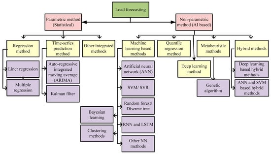
Figure 14.
Different methods used for load forecasting using smart metering system.
9.1. Parametric Methods
Parametric methods are the regression-based methods which perform forecasting based on various regression techniques. In parametric methods, fixed parameters are used to model load forecasting. It is applicable for linear relationships among variables and works on normal distribution.
9.1.1. Regression Methods
The regression methods are based on regression analysis in which a relationship exists between dependent variables and more than one independent variables. They are further classified as linear regression and multiple regression.
Linear Regression
Massidda et al. [181] addressed the load forecasting scheme using smart meters from different time horizons for both deterministic and probabilistic forecasts. Studies are conducted over time horizons ranging from one minute to one year. This method uses hybrid models that combine random forest (RF) and linear regression (LR), where RF is used for long-term forecasts and LR is used for short-term forecasts. In probabilistic forecasts, a household load was used. The dataset contained 2,075,259 measurements taken from a house in Sceaux (near Paris) from December 2006 to November 2010 (47 months). The first three years of the data were used for training, and the last year was used for validation. In order to assess the effectiveness of the method, MAE and RMSE were calculated for different time horizons. The RMSE for different time horizons were 0.648 kW, 0.704 kW, 0.604 kW, and 0.145 kW.
Goude et al. [182] proposed a semi-parametric model for forecasting electricity demand in France’s distributed network. The proposed method is used for short-term day-ahead and medium-term year-ahead load forecasting. In this case, the semi-parametric model is based on generalized additive models, which are statistical models. In accordance with the proposal, researchers collected data about electricity load every 10 min from 2260 substations through ERDF (Électricité Réseau Distribution de France). In the proposed theory, the relationship between load and other variables such as temperature, calendar variables, etc., could be determined.
Multiple Regression
Hayes et al. [183] proposed a multi-nodal STLF based on multiple linear regression using smart meter data. For load forecasting, load consumption statistics and weather data are taken. Data were analyzed from two regions, the Danish distribution network and the Irish distribution network. In the Danish network, the one-hour data of 1400 consumers were collected from 2012 to 2014 (24 months), while the Irish network collected the half-hour data of 6500 consumers for 18 months. It was shown in this study that load forecasting was carried out at multiple nodes in the opted network. This study compared an existing top-down forecasting approach with a bottom-up forecasting approach. The model’s accuracy performance was determined by calculating MAPE.
Ding et al. [184] proposed a time series load forecasting model using real-time measurements from smart meters. Using this model, the load power consumption is divided into three components: the trend component, the cyclic component, and the random error component. A multiple regression analysis is performed to estimate the trend component. The load data are then detrended into stationary series to determine the cyclic component using Fourier component regression. A simulation of the proposed model was conducted using data from the low voltage/medium voltage substations of the French distribution network.
9.1.2. Time Series Prediction Method
In time series analysis, the data points are analyzed at fixed intervals or consistently over time. In this method, the forecasting is done based on previously mentioned values. In the following sections, we discuss smart metering-based time series prediction in more details.
ARIMA Method
Alberg et al. [185] proposed a sliding window-based algorithm for STLF based on energy consumption data from smart meters. Using online information network incremental learning methodologies, these algorithms integrate seasonal and non-seasonal time series S(ARIMA) models. In this instance, the incremental ARIMA model is used to continuously access incoming time series load data every hour or every day. In the proposed scheme, two dynamic ARIMA algorithms were implemented, one seasonal, one non-seasonal, and they were tested on six smart meter data for a period of 16 months.
Twanabasu et al. [186] presented an hourly basis short-term load forecasting in smart grid-oriented buildings. To accomplish this, three forecasting techniques were modeled: ARIMA, ANN, and SVM. The hourly historical data of Ostfold University College in Halden, Norway from 2008 to 2010 were collected and fed into the three methods. When comparing the three methods based on MAPE, ARIMA shows 5.67% forecasting accuracy, ANN shows 5.31%, and SVM shows 7.68%. As a result of its good transparency, ARIMA was eventually selected as the STLF model.
Kalman Filter
The Kalman filter is a recursive algorithm which is used for load forecasting [187]. It has been noted that for long-term load forecasting, there exist various uncertainties due to seasonal and socioeconomic factors. This effect increases the error up to 10% or more. Therefore, by applying Kalman filters, we can reduce the error [50]. The Kalman filter is also known as a linear quadratic estimator that uses time series measurements.
Ghofrani et al. [187] presented a STLF based on the Kalman filter method. The smart meter data are extracted from the consumers in real-time and include both the actual energy consumption value and the Gaussian noise signal. In spectral analysis, Gaussian noise signals are filtered out. A Kalman filter is then applied to forecast the load. The method was evaluated using data collected over 15 min, 30 min, and an hour. A MAPE-based calculation was used to determine accuracy.
9.1.3. Other Integrated Methods
Hayes et al. [177] presented a local level STLF by using various linear and non-linear models. According to their analysis, the load demand was correlated with various other variables in the forecasting process. A variable is defined as a set of data that is related to the environment (such as the temperature, humidity, solar radiation, wind speed, etc.) and time (hour, day, hour of day, etc.) and historical data. A study was conducted on the dataset collected from smart meters in Danish and Irish power distribution networks. A variety of regression techniques were used for forecasting, such as a Naive model, a load shape model, a linear autoregression model, and a non-linear autoregression model. By calculating the MAPE for each model, a comparison was made among the models.
9.2. Non-Parametric Methods
Non-parametric methods are also known as AI-based models. They are flexible in modeling load forecasting models with a number of parameters. This works for non-linear relationships among the variables. It requires more data than parametric methods. The types of non-parametric methods are described below.
9.2.1. Machine Learning-Based Methods
The neural network methods are a subset of machine learning models. As described in the above section, it is similar to the operation of a human brain. There are various layers through which the data is trained. A review of the ML-based methods is described below.
Artificial Neural Network
Shahzadeh et al. [178] proposed a smart meter data-based load forecasting method using the information collected from individual residential users. In order to forecast, each cluster of users is divided into several clusters, and then ANN is used to train each cluster. Forecasting at the cluster level is then summed up for aggregate load forecasting. In order to collect suitable data, 6000 smart meter records from consumers in Ireland were used, of which 3176 records were selected for analysis. A dataset was taken for the period 14 July 2009 to 31 December 2010.
Asare-Bediako et al. [188] proposed a residential level day-ahead load forecasting method using ANN model. The smart meter data are used to extract the data for the training purpose. Aside from the load consumption, weather data (temperature and humidity) are considered, along with various time horizons (hour, minute, weekend, and holiday). Analysis was done on two months of data starting on 24 December 2009 and ending on 27 February 2010.
Sulaiman et al. [189] presented day-ahead load forecasting based on SMs data. ANN is used for forecasting an hourly load from the household customers. Apart from load consumption, weather-related data are taken into account both inside and outside the home. The datasets from 1 May 2012 to 31 July 2012 were used for experimental analysis, with 80% of the data being used for training and the remainder being used for testing. The overall accuracy of 70.54% was obtained with the proposed method.
Khan et al. [190] addressed the load forecasting of variable customer load using SMs. The load consumption of the customers varies according to a number of factors. There is a potential for forecasting inaccuracy because of this variable load. Hence, K-means clustering is used for clustering load consumptions in order to overcome this issue. Hence, different categories of loads are categorized separately, and then forecasting is performed over each one. ANN models are used as forecasting models, utilizing back propagation algorithms for learning. A study of the model was performed on the trials of Irish smart meters, where more than 5000 consumers were enlisted and a reading was taken every 30 min for every consumer. As input to the learning module, load consumption datasets, weather variables, and time horizon variables were considered. By using absolute mean error (AME), MAPE, and daily peak MAPE, the parameters of the model were evaluated.
Wang et al. [41] proposed an ensembled load forecasting model using SMs data. A multiple forecasting approach is implemented in the ensemble approach in order to obtain multiple forecasts. The first step in this methodology is clustering the various profiles into many subgroups. Forecasting is performed on each of the sub-groups individually using ANN models. In order to provide the final forecast, all subgroup forecasts are compiled using the optimal weight ensemble method. From 20 July 2009 to 26 December 2010, Irish residential smart meter data of more than 5000 users were collected for the study, and the RMSE and MAPE of the method were determined to be 3.83% and 4.71%.
Ponocko et al. [180] presented a load forecasting scheme on a residential level by using SM data. To forecast the load, first they ungroup the household load into various homes, each with its own main meter and sub-meter that has two levels of metering. ANNs are used to train household equipment-specific data at the submeter level. As the ANN is trained, it forecasts the total W and VAR power at a common assigned point and provides weighting factors for each load category. It is, thus, possible to achieve the total forecasting. Based on SM data, a study of the model was conducted on around 1000 consumers with occupancy in the United Kingdom (UK).
Oprea et al. [42] presented an STLF based on a machine learning algorithm using a smart meter dataset. First, the dataset is collected and stored in a nonstructured query language (NoSQL) database along with the meteorological variables. The analysis of these datasets is conducted to determine the most appropriate dataset for load forecasting. In the next step, k-means clustering is used to group similar characteristics of the dataset according to consumption types. In order to forecast cluster-wise loads with these data, feedforward ANN (FF-ANN) is used as a training method. Datasets were collected on 114 residential consumers in New England from June 2014 to December 2015. We compared the model with other machine learning algorithms and evaluated the accuracy by calculating the RMSE for each algorithm.
SVM/SVR
Gajowniczek et al. [13] proposed STLF by taking the smart meter data of each individual user. In their proposal, support vector machines and multi-layer perceptron feedforward neural network methods are used to implement the method. In their study, a smart meter was installed in a house with two adults and one child. All necessary household appliances were installed in the users’ house, and 60 days’ worth of data were collected. In order to validate the proposed method, the precision between forecasted load and actual load was calculated. Precision is measured by mean squared error (MSE). Results showed that both MLP and SVM models were capable of good forecasting with low error rates.
Aung et al. [191] introduced an approach for forecasting the daily peak load of individual SMs. In order to forecast load, the least squares method is used with SVR. To forecast the peak load, authors took into consideration the previous day’s peak load, the previous day’s average temperature, and the previous day’s holiday status. As part of the experiment, Germany’s Lower Saxony (LS) region and North Rhine-Westphalia (NRW) region were analyzed through smart meters. Among both regions of Germany, the smart meter dataset from 1 February 2009 to 30 June 2009 was used for training the least square SVR model, while the dataset from 1 July 2009 to 31 December 2009 was used for testing.
Humeau et al. [192] presented a load forecasting method for household consumers using various machine learning methods. SVR and multilayer perceptron (MLP) were used for machine learning. The 30 min load consumption data from over 5000 homes in Ireland from 2009 to 2010 were taken into consideration, provided by the Irish Smart Metering system (Commission for Energy Regulation). Data for the first 12 months were considered for training, and data for the remaining 6 months were considered for testing. In order to evaluate ML-based methods, MAPE and RMSE were calculated.
Vrablecová et al. [193] introduced a STLF using an online SVR method. Forecasting using SVR is advantageous because it handles non-linear time series accurately. A model for online SVR is considered here, which has the same performance characteristics of a conventional SVR model. Smart meters installed by the Commission for Energy Regulation (CER) in Ireland were used to collect the dataset for evaluation. More than 5000 consumers’ data were collected from 2009 to 2010 at a 30-min intervals. More than 5000 data were collected during the pre-processing stage, but only 3639 were gathered based on the pre-processing. The model’s performance was evaluated by calculating the MAPE.
Zhang et al. [194] proposed STLF based on big data technology using smart energy meter consumption data. The first step in this article is to identify the load pattern of different loads by clustering them. As another step, association analysis is used to determine the influencing factors, such as temperatures, humidity, and day types. The next step is to classify the data using decision trees. In order to forecast load, a SVM model must be selected based on a number of factors including load patterns and critical factors. Afterwards, individual loads are forecasted, and system loads are forecasted based on the sum of each individual forecasted load.
Random Forest and Discrete Tree
Pirbazari et al. [195] presented a new method for STLF by evaluating the feature selection methods. A variety of feature selection methods (F-regression, Mutual Information, Recursive Feature Elimination, and Elastic Net) are used to extract household load consumption from smart meters. The evaluation of these methods is done by using a predicting method, using the Gradient Boosted Regression Tree method. Data were collected from the smart meters of 23 houses in Norway from February 2017 to April 2018 in the time interval of 10 s. The RMSE was 4.80% for the proposed method.
Goehry et al. [196] proposed a ML approach for the forecasting load for a group of consumers. Groups of consumers are further divided into subgroups. In each subgroup, forecasting is performed by a random forecast algorithm. The forecasting at the sub-group level is consolidated to forecast the system load at the main group level or at the overall level once the forecasting is completed. An analysis of the model was conducted using Irish smart meter load data from 4225 consumers at every half hour in 2010. To check the accuracy of the model, the RMSE was calculated at the end, which was obtained as 25%.
Yu et al. [197] introduced a load forecasting method using a gradient boosting decision tree (GBDT) method using smart meter data. Buildings are equipped with smart meters that collect load consumption data and store it in the cloud server. Using the GBDT, the fitting function, loss function, decision tree model, and gradient descent function are integrated. Data were collected from smart meters in Huatuo from October 2018 to December 2012 using hourly readings. MAPE, normalized root mean square error (NRMSE), and coefficient of determination (R-square) were used to evaluate the performance of the method. This model was compared with NN and DT methods, and it showed that it is more reliable and suitable for load forecasting than the other methods.
RNN and LSTM
Sehovac et al. [198] presented a sequence-to-sequence RNN (S2S RNN) method for electric load forecasting. In this model, the S2S is used to model time dependencies load forecasting, and RNN is used to extract the time dependencies from load data. S2S is further used to strengthen the forecasting model by integrating two RNNs, such as encoder and decoder. The attention process is used to enhance the burden to connect encoders and decoders.
Fekri et al. [46] proposed a novel scheme for load forecasting considering smart meter data using online adaptive RNN. An online forecasting system is used. Using the offline learning method, once the model has been trained, it makes predictions about the load in the future. As a result, there is no chance to add new data to the already trained dataset. Hence, this paper proposes a continuous online learning process that can integrate new data into the model over time. The model was tested on five houses and found to be accurate when compared to other methods (MLP, linear regression, passive-aggressive regression, bagging regression, and K-nearest neighbor regression).
Jiao et al. [199] proposed an LSTM method for non-residential consumers using multiple correlated sequence information. In the first step, a multiple sequence RNN is used for load forecasting. The daily load curves of users are related to adjacent times, days, and weeks. In order to analyze the consumption pattern of consumers, K-mean clustering is used to cluster their daily load curves. After that, Spearman’s correlation coefficient is used to calculate consumer time series correlation. The LSTM then selects multiple time series to input into the model. An assessment of the implemented method is based on three indicators: MAE, RMSE, and MAPE. The minimum values obtained in the study were 23.84 KW, 22.45%, and 36.07 KW.
Kong et al. [200] demonstrated a residential load forecasting method based on the LSTM-RNN model. First, the clustering of a dataset is performed by a density-based clustering model to evaluate dissimilarity between aggregated and individual loads. The LSTM-RNN model is then introduced to the forecast load. During the period 01-Jun-2013 to 31-Aug-2013, a dataset was collected in New South Wales, Australia, with the training data gathered between 01-Jun-2013 and 05-Aug-2013. Validation of the dataset took place between 06-August-2013 and 22-August-2013, and testing took place between 23-August-2013 and 31-August-2013.
Razavi et al. [201] presented an innovative approach for STLF at the residential level based on smart meters. A multi-input single-output (MIMO) model based on LSTM is proposed here. An analysis of the effect of photo-voltaic (PV) generation on load forecasting is presented in this article. For consumers who have rooftop PV generation in their homes, grid power is also used to power their loads. In such cases, due to solar radiation impacting PV generation suddenly in the morning and evening, forecasting at these times can be challenging. For this condition, higher resolution data is needed, such as data collection at a time resolution of 5 min. The learning of the dataset was conducted using LSTM and MIMO-LSTM methods.
Imani et al. [202] presented a residential level load forecasting using an LSTM technique. Using a variable vector with lagged load, feature extraction is performed at every point along the load curve by the new method. The discrete wavelet transformation is applied on each variable vector to remove the high frequency components, which contain redundancies and noise (outlier). In the next step, the variable vectors are fed into a deep learning algorithm. Here, LSTM is considered a deep learning model for modeling the load forecasting model. An experiment was conducted using energy consumption data of 30 min taken from the smart meter of a residential customer in Canada. The proposed model was evaluated by MAPE, MAE, and MSE.
Bayesian Learning
The Bayesian method is used to work with time series data for load forecasting [203]. The Bayesian method has the property of variability, is non-stationarity, and is capable of processing with high uncertainties. Due to the features of the Bayesian method, it is widely used in machine learning [204].
Roth et al. [203] proposed a residential level building load forecasting using a Bayesian Structural Time Series (BSTS) model. The data are collected from the smart meters installed on apartment levels. Based on these datasets, features are selected using the spike and slab approach. Besides load consumption data, the model also includes variables like weather effects, holidays, and other dynamic factors. The proposed BSTS model has three applications: (1) load forecasting for aggregated apartment load, (2) submeter forecasting for multiple loads, and (3) measurement and verification of behavioral demand response for determining the saving effect. Using the smart meter data and submeter data of 120 apartment properties in Singapore, the BSTS model was studied. These data were collected from March 2018 to August 2019 by installing plug load sensors at each apartment. These plug sensors were categorized according to the household appliances in seven categories.
Yang et al. [204] presented a probabilistic load forecasting using the Bayesian deep learning method. At first, data are gathered from smart meters installed at each customer’s house. Based on the load consumption, these data are then clustered into different groups. The clustering-based pooling model is designed for the better utilization of data in the training phase. The training and learning for the forecasting is done using the Bayesian deep learning (BNN) method. Two types of smart meter datasets were collected for the study: the Irish Commission for Energy Regulation (CER) and the Australian Smart Grid Smart City (SGSC) project. In CER, data were collected from July 2009 to December 2010 for 4225 residential customers and 2210 small and medium-sized businesses. In contrast, data for the SGSC were collected for 10,000 customers from 2010 to 2014. In order to evaluate the accuracy of the implemented method, the RMSE and MAE were calculated for each category of dataset and were obtained as 0.735 kWh, 0.441 kWh and 0.813 kWh, 0.521 kWh.
Clustering Methods
Al-Wakeel et al. [205] presented a load forecasting strategy using k-means clustering using SM load data. The focus of this paper is on the preliminary analysis and grouping of datasets while clustering is used for the forecasting algorithm. In this case, different profiles of loads are grouped together so that they belong to the same cluster. The k-means clustering technique is used for this purpose. Irish Smart Metering Customer Behaviour Trials (CBT) data were collected over 18 months from 1 July 2009 to 31 December 2010 for the purpose of experimentation. In order to determine the error between forecasted and actual values, RMSE and MAPE were calculated.
Yildiz et al. [206] studied the load forecasting model of household consumptions using a smart meter-based model. The authors proposed the clustering, classification, and forecasting (CCF) technique as a technique for day-ahead forecasting. The original 48-day time series point of load data is used to represent each day. Each period of a day is divided into five based on its mean, minimum, maximum, and standard deviation. As a result, 20 variables are now defined for each day instead of 48. Here, K-means clustering is used to cluster the various group profiles. The model incorporates smart meter consumption data as well as weather data and temporal information. The clustered load profiles are correlated with weather and temporal data using the classification and regression tree (CART) method. After this, training and testing of clustered data are done.
Imani et al. [207] proposed a forecasting model using the clustering method. Using this model, the features are categorized in two categories: first, the features obtained from customers’ load consumption curves, and second, the answers to various questionnaires. In the first category, a half-hour load data of individual customer is was (i.e., a total of 48 readings). Each day was divided into three parts and each part contained 16 data values. Hence, for each day, the average value for each part was calculated. This provided a week data of 3 × 7 = 21 features for a single customer. For the clustering method, K-means clustering was used. Performance was evaluated by calculating the MAPE as 3.71%.
Other NN Methods
Quilumba et al. [40] proposed a method for intraday load forecasting using smart meter data. To improve load forecast accuracy, this method is introduced. First, K-means clustering is used to cluster similar groups of customers in this paper. Second, based on clustering, load forecasting is done using the Levenberg–Marquardt model. At last, the individual load forecasting results are then integrated into the system forecast. The real-time dataset of users in New York and Ireland was taken into consideration here. In New York, 15-min load consumption data were collected from February 2012 to October 2013, from which the first 12 months’ datasets were used for training the model and the remaining sets were used for testing. A similar collection of 30 min of data were available for Ireland from 14 July 2009 to 31 December 2010. The MAPE were calculated as 0.5% and 1.07%.
Kell et al. [208] focused on the STLF using residential SMs data. Based on the data collected, K-means clustering is used to segregate and group each group of customers. In order to forecast the loads based on these clusters, various forecasting algorithms are implemented, such as random forecasting, NN, LSTM-NN, and SVR models. A comparison of the forecasts from different models was performed and it was evident that random forest performed better than all the other models for all clusters. The data for the simulation were collected from 5000 Irish customers over a time horizon of 30 min.
Taieb et al. [209] have proposed a quantile regression method for the probabilistic forecasting of household load consumption. The quantile regression method is classified under the non-parametric model of load forecasting. Datasets were collected from the Commission for Energy Regulation (CER) in Ireland, which focused on 4225 households and 2210 small to medium enterprises. There are 4225 dataset, 3639 of which were filtered out for consideration, and the remaining had missing values, so they were not considered. For the model, 30-min data between 14 July 2009 and 31 December 2010 were taken.
Peng et al. [210] discussed a STLF using machine learning methods for residential and small and medium enterprise (SME) customers. Various machine learning methods such as linear regression, gradient-boosted regression tree (GBRT), LSTM, SVR, and MLP are used for forecasting the loads. For the evaluation of the proposed method, MAE, RMSE, and MAPE were calculated and compared for the best one. Smart meter datasets were taken from the Commission for Energy Regulation (CER) in Ireland, from which 5000 customers in residential homes and SME between 2009 and 2010 were considered. For modeling purposes, 1700 homes and 250 small and medium-sized businesses were finally considered.
Heghedus et al. [211] proposed a load forecasting scheme using a deep learning model. Here, gated recurrent unit (GRU) is used to forecast the load. The SM data in terms of energy were collected for 4 months. For experimentation, the 10-sec data logged by SM were used. By calculating the MAPE of the proposed model, the performance was evaluated.
Rai et al. [212] presented a short-term and medium-term load forecasting based on various ML algorithms. The data are collected from the smart meters installed in various locations. The datasets are first pre-processed by using Gaussian filters to filter out suitable information. The machine learning techniques such as multiple linear regression (MLR), ANN, Holt’s exponential smoothening method, and SVR are used for STLF and MTLF. To evaluate forecasting methods, a case study of the National Institute of Technology Patna is presented. A SM was installed at each of the 15 nodes on campus, which took readings every five minutes. All forecasting methods were assessed using MAPE and RMSE, and it was found that SVR performed the most accurate forecasting among all methods. The values of MAPE and RMSE were 3.06% and 0.025.
Guo et al. [213] introduced a different stage of aggregated load forecasting using smart meter load data. In recent years, a number of researchers have proposed forecasting at the sub-metering level and then aggregating all such forecasts in order to forecast the overall load. As an alternative, Guo et al. proposed using the aggregated active power data for the total household load from the main smart meter. In this, an Explicit Duration Hidden Markov Model with differential observations (EDHMM-diff) is proposed for determining the individual appliances’ load from aggregated active power recorded by the SM. For the training and learning of the dataset, the forward–backward algorithm was used to forecast the load.
Grmanova et al. [214] proposed a model for time series load forecasting using an incremental heterogeneous ensemble method. In this article, the time series prediction is made along with concept drift. In this case, concept drift may be permanent or temporary (changes caused by economic factors or environmental factors) or seasonal (changes influenced by the weather and other factors such as daylight or wind speed). Various time series algorithms such as autoregressive, feedforward neural network, Holt–Winters exponential smoothing, seasonal decomposition by time series by loss, ARIMA, seasonal naive method-random walk, double seasonal exponential smoothing, and naive average long-term methods were compared for various results. The MAPE was found to be around 1.5%.
Fernández et al. [215] presented a STLF using privacy-preserving federated learning (FL) for residential customers. In this novel method, the authors used FL, which has the advantage of training different machine learning models simultaneously utilizing each other’s datasets, but without exposing any of their individual datasets. As a result of these activities, FL produces more accurate forecasts than an individual model. In order to perform the analysis, a half-hour load dataset from 5567 residential users in London (LCL dataset) was collected for the analysis. For training purposes, the January to December 2013 dataset was considered, and for testing purposes, the January to March 2014 dataset was considered. The MSE, MAE, MAPE, and RMSE of the proposed model were calculated for evaluation.
In [216], fuzzy logic-based residential load forecasting was performed. Input to the FIS model were temperature, occupancy, and week or special day. For forecasting, the residential load of a building in Memphis, USA, was considered. FIS was compared with an ANN model, and the result showed that the fuzzy method (14.34%) had a better MAPE than the ANN method (19.09%).
Li et al. [217] contributed towards STLF using smart meter data based on online sequential extreme machine learning (OS-ELM) algorithms. As a first step, the data are gathered and divided into various clusters based on various variables (workdays, holidays, and the day before holidays). In order to forecast the load, each cluster is forecast separately, and the overall forecast is generated by adding up all the cluster-wise forecasts. Data were derived from each 30-min period between 14 July 2009 and 31 December 2010 from the Irish Social Science Data Archive (ISSDA). The data were collected from 3000 residential consumers. The performance of the model was evaluated by calculating the MAPE.
9.2.2. Quantile Regression Method
Wang et al. [218] presented a new probabilistic aggregated LF algorithm using SM data. Data collected from SMs are first clustered to various groups using k-means clustering, spectral clustering, agglomerative clustering, and Gaussian mixture models (GMMs). Each group is then forecasted using SVR, gradient boost regression (GBR), and random forest regression (RFR). As a result, it obtains 12 forecasts using four models of clustering and three models of individual forecasting. Lastly, the probabilistic forecasts are obtained by assembling all the individual point forecasts. For the ensemble forecast, the methods Quantile Regression Averaging (Q-RA), Factor Quantile Regression Averaging (FQRA), LASSO Quantile Regression Averaging (LQRA), and Quantile Gradient Boosting Regression Tree (QGBRT) are proposed. Models were evaluated using the CER dataset of over 5000 residential consumers from an Irish region between 20 July 2009 and 26 December 2010.
Zhang et al. [219] introduced a new method for day-ahead load forecasting using various quantile forecasts. In this method, forecast is reached through the transformation and combination of quantile methods. Under the transformation, the kernel density estimation method is used to convert individual quantile forecast into a probability density forecast (PDF), whereas in the next step, weighted combinations of various PDFs are established to optimize the forecasting model. The multiple quantile forecasting is classified into five methods: Q-LR, Q-RF, QGBRT, Q-LGBM, and Q-GRU. The study of the discussed method was tested on load consumption in real-world data of the Guangdong province in China, ISO, New England (ISO-NE), and Irish smart meter data. The accuracy for both the provinces were obtained as 1.54% and 2.9%.
9.2.3. Metaheuristic Methods
Niska et al. [220] focused on the optimization of the parameters of NN for STLF using the GA optimization technique. The training of datasets is performed using MLP and SVM. Initially, the datasets are pre-processed in order to eliminate outliers before training. The features of the data are extracted and optimized through GA, and the appropriate dataset is fed to the algorithm for learning. In order to perform the analysis, hourly load consumption data were recorded for 3516 users between 2009 and 2010, with data from 2010 being used for training and data from 2009 being used for testing. In addition to the load consumption data, temperature values were also considered when training the models. The MAPE for daily and hourly resolution were obtained as 2.05% and 3.06%.
9.2.4. Deep Learning Methods
Hosein et al. [221] studied STLF based on DNN using smart meter load consumption data. The dataset is based on one-year load consumption by residential consumers through smart meters. Here, the datasets are split into weekdays and weekend days. The data are trained using deep neural networks such as the Deep Neural Network without pretraining (DNN-W), DNN with pretraining using Stacked Autoencoders (DNN-SA), RNN, and RNN-LSTM. A comparison of proposed DNN models with traditional methods was conducted. For the evaluation of DNN models, MAPE and mean percentage error (MPE) were calculated.
Shi et al. [222] presented a deep learning-based household load forecasting using smart meter data. In this model, a new pooling-based deep RNN is proposed, which eliminates the phenomenon of overfitting during the training of a neural network. Here, the different load profiles of groups of consumers are divided into pools of inputs. A dataset from Irish residential consumers of more than 5000 participants was used. The data were taken from 1 July 2009 to 31 December 2010. The model was compared with ARIMA, RNN, SVR, deep recurrent NN (D-RNN), and pooling-based D-RNN (PDRNNs) models. The accuracy of the proposed model exceeds the ARIMA, SVR, and D-RNN by 19.5%, 13.1%, and 6.5%.
Li et al. [223] introduced an IoT-based deep learning model for electricity load forecasting using smart meter data. The feature is extracted automatically by the method. The historical dataset of seven years from 2010 to 2016 in south China was collected for testing the model. Here, first the daily load forecasting was designed and then, based on this, intra-day load variations were forecasted. The deep learning methods were used to learn the patterns of the input dataset.
9.2.5. Hybrid Methods
In hybrid methods, a combination of two or more methods is used to forecast loads. When compared to a single method, hybrid methods provide a higher level of accuracy.
Deep Learning-Based Hybrid Methods
Khatri et al. [224] presented an STLF based on deep learning models. Simple RNN, gated recurrent unit (GRU), and LSTM are considered for deep learning algorithms. Data were taken from the smart meters of 6445 consumers from the Irish Social Science Data Archive (ISSDA) between 14 July 2009 and 31 December 2010. The performance of DNN models were evaluated by MAE, mean-square error (MSE), and root mean squared logarithmic error (RMSLE).
Fahiman et al. [32] introduced a new method for STLF using clustering and deep learning methods. Here, k-shape clustering is used to segregate the consumers into various clusters based on the different patterns of electricity consumption. The k-shape clustering is more accurate than k-means clustering. For deep learning methods, multilayer perceptron (MLP) and a restricted Boltzmann machine (RBM) are used for load forecasting and comparative analysis is performed for better prediction accuracy. The dataset was taken from 6000 smart meters of Irish consumers which provided 30-min resolution between 14 July 2009 and 31 December 2010.
Alhussein, et al. [225] proposed a hybrid model based on deep learning method for STLF using smart meter data. The deep learning model is based on CNN and LSTM, where CNN is used for the extraction of features and LSTM is used for the learning process. The datasets were collected from 10,000 smart meter consumers of the Australian Government project of Smart Grid Smart City (SGSC). Finally, MAPE was calculated for CNN-LSTM for performance evaluation. The proposed method showed a MAPE of 44.76% with the clustering approach, whereas it showed 44.68% with the LSTM approach.
Semmelmann et al. [226] proposed a hybrid model for residential level load forecasting based on LSTM-XGBoost model. In order to train the LSTM model, feature permutation is used to extract the required features. In this case, LSTM offers accurate forecasting of the entire community’s load. A model based on extreme gradient boost (XGBoost) is used to forecast the peak load time and value individually. Finally, the forecasted models are combined to produce an integrated forecast of community load. The dataset was gathered from the German smart meter household data for 130 residential users in 2019. The performance was evaluated by calculating MAPE and RMSE. The MAPE achieved was 17.99%.
Fekri et al. [227] presented a load forecasting scheme using a federal learning method collecting the load data from smart meters. An LSTM is used to initialize a model’s global weight. A subset of SMs is created for training purposes and the server provides a global model to selected SMs. The SM devices are trained with the local data. The local data are first pre-processed to suitable datasets and then trained by LSTM. Additionally, these pre-processed data are trained using federated stochastic gradient descent (FedSGD) and federated averaging (FedAVG). After this, the trained SM devices send the new parameters to the server. As soon as it receives the new parameters from the server, it sums them up to obtain a more accurate global model. The integration can be achieved using FedSGD and FedAVG. When the models intersect, all participants are trained on the global model. Following this, these participants replace their old local models with the new updated ones from the server and perform a load forecast. An experiment using the FL was conducted on smart meter data provided by London Hydro, from which 19 consumers with one-hour readings were evaluated over a three-year period. Hence, with a total of 25,560 consumers, 485,640 readings in total were collected. The evaluation of the model was performed by calculating MAPE and RMSE values.
Ünal et al. [228] presented a hybrid approach based on deep learning methods utilizing SMs data. CNN and bidirectional LSTM (BLSTM) models are used in deep learning methodology. This article mainly focuses on the advanced pre-processing of data which are collected from smart meters. To achieve this, SMs first clean the data by eliminating missing values and then detect outliers that are recorded as false readings. Using clustering-based algorithms, outliers can be better detected. Secondly, they use density-based clustering algorithms for detecting irregularities in daily load profiles. After the advanced pre-processing of data, the training of the obtained data is accomplished by hybridization of the CNN and BLSTM models. The study of the proposed method was performed on the real-life SM load data collected from different customers in Turkey. A total of 56 residential and 44 commercial users were considered, from which 28,876 daily consumption readings were recorded. After the advanced pre-processing, these values were filtered out to 22,506. The dataset for 2018 was collected for the study. The performance of the method was evaluated by calculating RMSE, MAE, MAPE and normalized RMSE (NRMSE). The MAPE for different time horizons were obtained as 36.748%, 36.911, and 38.008%.
Singh et al. [229] introduced load forecasting methods for a distribution transformer. They used IoT-based smart meters for the collection of data. The authors presented two very different approaches for forecasting. The first approach creates parametric estimation for every individual model according to the day of the week. The second approach ensures that the model can be developed irrespectively of the day of the week. The model of maximum correlation coefficient is selected based on the previous patterns of the previous few hours of the day. Here, the total load consumption is modeled by LR, SVR, and NN. For studying the model, the load consumption recorded by smart meters of 6000 consumers were taken from the Irish distribution network. The NN models provided a mean error of 7%.
ANN- and SVM-Based Hybrid Methods
Khan et al. [230] utilized smart meter data for load forecasting, and demand side management. Data collected from SMs are clustered. The forecasting is performed using feedforward ANN and multiple linear regression (MLR). During the forecasting process, weather variables, load consumption data, and calendar data are taken into account. The study used data from more than 5000 smart meters in Ireland (ISSDA) every half hour. Validation of the proposed method was performed by calculating MAPE.
10. Conclusions and Future Scope
In this paper, a detailed report of various load forecasting methods conducted using conventional and smart meter information are articulated. Forecasting for all types of loads has been widely discussed, including very short-term, short-term, medium-term, and long-term. A vast majority of forecasting models use smart meters to gather electricity load consumption data. In smart grids, these smart meters can be installed in a variety of locations depending on the data requirements. Researchers have shown interest in forecasting individual consumer loads and then summing them up for regional forecasts based on smart meter information. Many researchers directly use smart meter data from smart meters installed at the distribution end to forecast load region-by-region.
Generally, the forecast models are of two types: parametric and non-parametric. The parametric methods work with linear data forms, whereas non-parametric methods use non-linear data and are based on artificial intelligence. It is also observed that, apart from historical load data from smart meters, many techniques consider various inputs to their models, including weather data (temperature, humidity, wind speed, solar radiations, etc.) and time horizons. To determine the accuracy of the system, key performance indicators are used for each model.
A variety of electricity distribution networks have been studied, including the Irish distribution network, the Danish distribution network, the French distribution network, the Australian distribution network, residential electricity consumers in the UK, New England, Germany, Singapore, New York, China, various universities, and many more. Smart meters are used to collect the load consumption data from consumers.
Considering the present scenario of increased electricity demand, smart meters are a must for the smooth operation and handling of future smart grid. With such a facility, load forecasting should also be easier and accurate, to handle the future energy market. In addition, it will be possible to upload large and authentic datasets generated by smart meters directly to a server so that they can be analyzed more precisely.
Author Contributions
F.D.: Conceptualization, methodology, software, validation, formal analysis, and investigation; A.Y.A.: resources, data curation, and review and editing; M.B.: original draft preparation, review and editing, and supervision. All authors have read and agreed to the published version of the manuscript.
Funding
This research did not receive any specific grant from funding agencies in the public, commercial, or not-for-profit sectors.
Data Availability Statement
Not applicable.
Acknowledgments
The authors would like to acknowledge the Department of Electrical Engineering, National Institute of Technology, Raipur for providing all the facilities and support to conduct this research.
Conflicts of Interest
The authors declare no conflict of interest.
Abbreviations
| LF | Load forecasting |
| RNN | Recurrent neural network |
| LSTM | Long short-term memory |
| SMs | Smart meters |
| IoT | Internet of things |
| GSM | Global system for mobile communication |
| ML | Machine learning |
| VSTLF | Very short-term load forecasting |
| STLF | Short-term load forecasting |
| MTLF | Medium-term load forecasting |
| LTLF | Long-term load forecasting |
| KPI | Key performance indicators |
| EMD | Empirical mode decomposition |
| IMFs | Intrinsic mode functions |
| P-IMF | Principal-IMFs |
| SVP | Support vector regression for P-IMF |
| B-IMF | Behavioural-IMFs |
| SVB | Support vector regression for B-IMF |
| RBFNN | Radial basis function neural network |
| DEKF | Dual extended Kalman filter |
| SVR-DEKF-RBFNN | Support vector regression-dual extended Kalman filter-radial basis function neural network |
| RF | Random forest |
| DT | Discrete tree |
| SVR2 | SVR based on similar historical days |
| RW | Random walk |
| CART | Classification and regression trees |
| REPTree | Reduced error pruning trees |
| DS | Decision stumps |
| 1-D | 1-dimensional |
| DLNN | Deep learning neural network |
| S2S | Sequence to sequence-based LSTM |
| VMD | Variation mode decomposition |
| RBFN | Radial basis function neural network |
| XGBoost | eXtreme gradient boosting |
| FCRBM | Factored restricted Boltzmann machines |
| GRU | Gated recurrent unit |
| FS | Feature selection |
| BPDB | Bangladesh power development board |
| EPSO | Evolutionary particle swarm optimization |
| ANFIS | Adaptive neuro-fuzzy inference system |
| WLS | Weighted least squares state estimation |
| GA-BPN | GA based back propagation network |
| nGA | Novel genetic algorithm |
| MANN | Multilayer ANN |
| ENN | Elman neural network |
| GRNN | General regression neural network |
| BPNN | Back-propagation neural network |
| LS-SVM | Linear square-support vector machine |
| PSOSVM | Particle swarm optimization with support vector machine |
| ABC | Artificial bee colony |
| MAE | Mean absolute error |
| MAPE | Mean absolute percentage error |
| MSE | Mean squared error |
| RMSE | Root mean square error |
| RRSE | Root relative squared error |
| CV | Coefficient of variation |
| MLI | Maximum likelihood imputation |
| AR | Autoregressive |
| MA | Moving average |
| ARMA | Auto-regressive moving average |
| ARIMA | Auto-regressive integrated moving average |
| AI | Artificial intelligence |
| NN | Neural network |
| ANN | Artificial neural network |
| RNN | Recurrent neural network |
| CNN | Convolutional neural network |
| SVM | Support vector machine |
| SVR | Support vector regression |
| GA | Genetic algorithm |
| PSO | Particle swarm optimization |
| IEMD | Improved empirical mode decomposition |
| WNN | Wavelet neural network |
| FOA | Fruit fly optimization algorithm |
| GRA | Grey relational analysis |
| GM | Grey model |
| GBP | Grey model with back propagation |
| GP | Genetic programming |
| HOGM | Hybrid optimized grey model |
| WT | Wavelet transform |
| DNN | Deep neural network |
| MLP | Multilayer perceptron |
| STMLF | Short term multiple load forecasting |
| RBF | Radial basis function |
| DRNN | Decay RBF neural networks |
| ELM | Extreme learning machine |
| ISO | Improved second-order algorithm |
| ErrCor | Error correction algorithm |
| EANN | Ensemble artificial neural network |
| BANN | ANN based bagging model |
| SVRIA | Support vector regression with immune algorithm |
| LWR | Locally weighted regression |
| S(ARIMA) | Seasonal and non-seasonal time series ARIMA |
| AME | Absolute mean error |
| W | Active power |
| VAR | Reactive power |
| UK | United Kingdom |
| NoSQL | Non structured query language |
| FF-ANN | Feed forward ANN |
| LS | Lower Saxony |
| NRW | North Rhine-Westphalia |
| CER | Commission for Energy Regulation |
| F-regression | Feature regression |
| GBDT | Gradient boosting decision tree |
| NRMSE | Normalized root mean square error |
| MIMO | Multi-input single-output |
| PV | Photo-voltaic |
| BSTS | Bayesian Structural Time Series |
| BNN | Bayesian deep learning |
| SGSC | Smart Grid Smart City |
| CBT | Customer Behaviour Trials |
| CCF | Clustering, classification and forecasting |
| SME | Small and medium enterprises |
| GBRT | Gradient boosted regression tree |
| MLR | Multiple linear regression |
| EDHMM-diff | Explicit duration hidden Markov model with differential observations |
| FL | Federated learning |
| OS-ELM | Online sequential extreme machine learning |
| ISSDA | Irish Social Science Data Archive |
| GMMs | Gaussian mixture models |
| GBR | Gradient boost regression |
| RFR | Random forest regression |
| Q-RA | Quantile regression averaging |
| FQRA | Factor quantile regression averaging |
| LQRA | LASSO quantile regression averaging |
| QGBRT | Quantile gradient boosting regression tree |
| Probability density forecast | |
| Q- LR | Quantile linear regression |
| Q-RF | Quantile random forest |
| Q-LGBM | Quantile light gradient boost model |
| Q-GRU | Quantile gated recurrent unit |
| ISO | Independent system operator |
| SRSVRC-ABC | Seasonal recurrent support vector regression with chaotic ABC |
| IESO | Independent electricity system operator |
| RBF-NN | Radial biased function neural network |
| ACO | Ant colony optimization |
| CI | Computational intelligence |
| ACO-GA | Integrating ant colony optimization with genetic algorithm |
| IACC | Improved ant colony clustering |
| COR-ACO-GA | Cooperative ant colony optimization, genetic algorithm |
| FIS | Fuzzy inference system |
| AIS | Artificial immune system |
| AIN | Artificial immune network |
| DAIA | Improved artificial immune algorithm |
| RPE | Relative error |
| IN | Immune network |
| DBN | Deep belief network |
| NSW | New South Wales |
| DWT | Discrete wavelet transform |
| RVFL | Random vector functional link network |
| SDAs | Stacked denoising auto-encoders |
| LM | Levenberg-Marquardt |
| BP | Back propagation |
| ELF | Electrical load forecasting |
| ELMnn | Extreme learning machine neural network |
| MSsa | Multi-objective slap swarm algorithm |
| IA-FOA | Immune algorithm and fruit fly optimization algorithm |
| FOA | Fruit fly optimization algorithm |
| AAE | Average absolute error |
| HS | Harmony search |
| MFA | Modified firefly algorithm |
| FE | Feature engineering |
| mFFO | Modified fire-fly optimization |
| FE-SVR-mFFO | Feature engineering- support vector regression- mFFO |
| IAGA | Improved adaptive genetic algorithm |
| AMI | Advanced metering infrastructure |
| LR | Linear regression |
| ERDF | Électricité Réseau Distribution de France |
| DNN-SA | DNN with pretraining using Stacked Auto encoders |
| MPE | Mean percentage error |
| D-RNN | Deep recurrent neural network |
| PDRNN | Pooling-based D-RNN |
| RMSLE | Root mean squared logarithmic error |
| DNN-W | Deep neural network without pretraining |
| RBM | Restricted Boltzmann machine |
| FedSGD | Federated stochastic gradient descent |
| FedAVG | Federated averaging |
| BLSTM | Bidirectional long short-term memory |
| NRMSE | Normalized root mean square error |
References
- Lahouar, A.; Slama, J.B.H. Day-ahead load forecast using random forest and expert input selection. Energy Convers. Manag. 2015, 103, 1040–1051. [Google Scholar] [CrossRef]
- Rafati, A.; Joorabian, M.; Mashhour, E. An efficient hour-ahead electrical load forecasting method based on innovative features. Energy 2020, 201, 117511. [Google Scholar] [CrossRef]
- Debdas, S.; Mohanty, S.; Kundu, S.; Mohanty, S.; Biswas, B.; Pal, A. Short-Term Load Forecasting Using Time Series Algorithm. In Proceedings of the International Conference on Artificial Intelligence and Smart Systems (ICAIS-2021), Coimbatore, India, 25–27 March 2021. [Google Scholar] [CrossRef]
- Jain, R.; Mahajan, V. Load forecasting and risk assessment for energy market with renewable based distributed generation. Renew. Energy Focus 2022, 42, 190–205. [Google Scholar] [CrossRef]
- Liang, J.; Tang, W. Ultra-Short-Term Spatiotemporal Forecasting of Renewable Resources: An Attention Temporal Convolutional Network-Based Approach. IEEE Trans. Smart Grid 2022, 13, 3798–3812. [Google Scholar] [CrossRef]
- Jahan, I.S.; Snasel, V.; Misak, S. Intelligent Systems for Power Load Forecasting: A Study Review. Energies 2020, 13, 6105. [Google Scholar] [CrossRef]
- Kaur, A.; Pedro, H.T.C.; Coimbra, C.F.M. Impact of onsite solar generation on system load demand forecast. Energy Convers. Manag. 2013, 75, 701–709. [Google Scholar] [CrossRef]
- Soroudi, A.; Amraee, T. Decision making under uncertainty in energy systems: State of the art. Renew. Sustain. Energy Rev. 2013, 28, 376–384. [Google Scholar] [CrossRef]
- Dutta, S.; Li, Y.; Venkataraman, A.; Costa, L.M.; Jiang, T.; Plana, R.; Tordjman, P.; Choo, F.H.; Foo, C.F.; Puttgen, H.B. Load and Renewable Energy Forecasting for a Microgrid using Persistence Technique. Energy Procedia 2017, 143, 617–622. [Google Scholar] [CrossRef]
- Kaur, A.; Nonnenmacher, L.; Coimbra, C.F.M. Net load forecasting for high renewable energy penetration grids. Energy 2016, 114, 1073–1084. [Google Scholar] [CrossRef]
- Cecati, C.; Kolbusz, J.; Rozycki, P.; Siano, P.; Wilamowski, B.M. A Novel RBF Training Algorithm for Short-Term Electric Load Forecasting and Comparative Studies. IEEE Trans. Ind. Electron. 2015, 62, 6519–6529. [Google Scholar] [CrossRef]
- Barman, B.K.; Yadav, S.N.; Kumar, S.; Gope, S. IOT based smart energy meter for efficient energy utilization in smart grid. In Proceedings of the 2nd International Conference on Power, Energy and Environment: Towards Smart Technology (ICEPE), Shillong, India, 1–2 June 2018; pp. 1–5. [Google Scholar]
- Gajowniczek, k.; Zbkowski, T. Short term electricity forecasting using individual smart meter data. Procedia Comput. Sci. 2014, 35, 589–597. [Google Scholar] [CrossRef]
- Buonanno, A.; Caliano, M.; Pontecorvo, A.; Sforza, G.; Valenti, M.; Graditi, G. Global vs. Local Models for Short-Term Electricity Demand Prediction in a Residential/Lodging Scenario. Energies 2022, 15, 2037. [Google Scholar] [CrossRef]
- Januschowski, T.; Gasthaus, J.; Wang, Y.; Salinas, D.; Flunkert, V.; Bohlke-Schneider, M.; Callot, L. Criteria for classifying forecasting methods. Int. J. Forecast. 2020, 36, 167–177. [Google Scholar] [CrossRef]
- Montero-Manso, P.; Hyndman, R.J. Principles and Algorithms for Forecasting Groups of Time Series: Locality and Globality. Int. J. Forecast. 2021, 34, 1632–1653. [Google Scholar] [CrossRef]
- Taylor, J.W. An evaluation of methods for very short-term load forecasting using minute-by-minute British data. Int. J. Forecast. 2008, 24, 645–658. [Google Scholar] [CrossRef]
- Yang, H.Y.; Ye, H.; Wang, G.; Khan, J.; Hu, T. Fuzzy neural very short-term load forecasting based on chaotic dynamics reconstruction. Chaos Solitons Fractals 2006, 29, 462–469. [Google Scholar] [CrossRef]
- Kawauchi, S.; Sugihara, H.; Sasaki, H. Development of very-short term load forecasting based on chaos theory. Elect. Eng. Jpn. 2004, 148, 55–63. [Google Scholar] [CrossRef]
- Alamaniotis, M.; Ikonomopoulos, A.; Tsoukalas, L.H. Evolutionary multi-objective optimization of Kernel-based very-short-term load forecasting. IEEE Trans. Power Syst. 2012, 27, 1477–1484. [Google Scholar] [CrossRef]
- Migon, H.S.; Alves, L.C. Multivariate dynamic regression: Modelling and forecasting for intraday electricity load. Appl. Stoch. Model. Bus. Ind. 2013, 29, 579–598. [Google Scholar] [CrossRef]
- Guan, C.; Luh, P.B.; Michel, L.D.; Wang, Y.; Friedland, P.B. Very short-term load forecasting: Wavelet neural networks with data pre-filtering. IEEE Trans. Power Syst. 2013, 28, 30–41. [Google Scholar] [CrossRef]
- Hsiao, Y.H. Household Electricity Demand Forecast Based on Context Information and User Daily Schedule Analysis from Meter Data. IEEE Trans. Ind. Inform. 2015, 11, 33–43. [Google Scholar] [CrossRef]
- Soliman, S.A.; Al-Khandari, A.M. Dynamic electric load forecasting. Electr. Load Forecast. 2010, 291–352. [Google Scholar] [CrossRef]
- Baliyan, A.; Gaurav, K.; Mishra, S.K. A Review of Short-Term Load Forecasting using Artificial Neural Network Models. Procedia Comput. Sci. 2015, 48, 121–125. [Google Scholar] [CrossRef]
- Mamun, A.A.; Sohel, M.; Mohammad, N.; Sunny, M.S.H.; Dipta, D.R.; Hossain, E. A comprehensive review of the load forecasting techniques using single and hybrid predictive models. IEEE Access 2020, 8, 134911–134939. [Google Scholar] [CrossRef]
- Hambali, A.O.; Akinyemi, M.; JYusuf, N. Electric Power Load Forecast Using Decision Tree Algorithms. Comput. Inf. Syst. Dev. Inform. Allied Res. J. 2017, 7, 29–42. [Google Scholar]
- Hafeez, G.; Alimgeera, K.S.; Khanb, I. Electric load forecasting based on deep learning and optimized by heuristic algorithm in smart grid. Appl. Energy 2020, 269, 114915. [Google Scholar] [CrossRef]
- Abu-Shikhah, N.; Elkarmi, F. Medium-term electric load forecasting using singular value decomposition. Energy 2011, 36, 4259–4271. [Google Scholar] [CrossRef]
- Amjady, N.; Daraeepour, A. Midterm demand prediction of electrical power systems using a new hybrid forecast technique. IEEE Trans. Power Syst. 2011, 26, 755–765. [Google Scholar] [CrossRef]
- Wi, Y.M.; Joo, S.K.; Song, K.B. Holiday load forecasting using fuzzy polynomial regression with weather feature selection and adjustment. IEEE Trans. Power Syst. 2012, 27, 596–603. [Google Scholar] [CrossRef]
- Fahiman, F.; Erfani, S.M.; Rajasegarar, S.; Palaniswami, M.; Leckie, C. Improving load forecasting based on deep learning and K-shape clustering. In Proceedings of the International Joint Conference on Neural Networks (IJCNN), Anchorage, AK, USA, 14–19 May 2017; pp. 4134–4141. [Google Scholar] [CrossRef]
- Kumar, A.; Yan, B.; Bilton, A. Machine Learning-Based Load Forecasting for Nanogrid Peak Load Cost Reduction. Energies 2022, 15, 6721. [Google Scholar] [CrossRef]
- Aldegheishem, A.; Anwar, M.; Javaid, N.; Alrajeh, N.; Shafiq, M.; Ahmed, H. Towards sustainable energy efficiency with intelligent electricity theft detection in smart grids emphasising enhanced neural networks. IEEE Access 2021, 9, 25036–25061. [Google Scholar] [CrossRef]
- Zheng, Z.; Yang, Y.; Niu, X.; Dai, H.-N.; Zhou, Y. Wide and deep convolutional neural networks for electricity-theft detection to secure smart grids. IEEE Trans. Ind. Informat. 2018, 14, 1606–1615. [Google Scholar] [CrossRef]
- Dong, X.; Qian, L.; Huang, L. Short-term load forecasting in smart grid: A combined cnn and k-means clustering approach. In Proceedings of the IEEE International Conference on Big Data and Smart Computing (BigComp), Jeju, Korea, 13–16 February 2017; pp. 119–125. [Google Scholar] [CrossRef]
- Garcia, S.; Ramirez-Gallego, S.; Luengo, J.; Benitez, J.M.; Herrera, F. Big Data Preprocessing: Methods and prospects. Big Data Anal. 2016, 1, 9. [Google Scholar] [CrossRef]
- Lean Yu, L.; Zhou, R.; Chen, R.; Lai, K.K. Missing Data Preprocessing in Credit Classification: One-Hot Encoding or Imputation? Emerg. Mark. Financ. Trade 2020, 58, 472–482. [Google Scholar] [CrossRef]
- Garcia, S.; Luengo, J.; Herrera, F. Data Preprocessing in Data Mining (Intelligent Systems Reference Libraray); Springer: Berlin/Heidelberg, Germany, 2015; p. 72. [Google Scholar]
- Quilumba, F.L.; Lee, W.-J.; Huang, H.; Wang, D.Y.; Szabados, R.L. Using Smart Meter Data to Improve the Accuracy of Intraday Load Forecasting Considering Customer Behavior Similarities. IEEE Trans. Smart Grid 2015, 6, 911–918. [Google Scholar] [CrossRef]
- Wang, Y.; Chen, Q.; Sun, M.; Kang, C.; Xia, Q. An ensemble forecasting method for the aggregated load with subprofiles. IEEE Trans. Smart Grid 2018, 9, 3906–3908. [Google Scholar] [CrossRef]
- Oprea, S.-V.; Bara, A. Machine Learning Algorithms for Short-Term Load Forecast in Residential Buildings Using Smart Meters, Sensors and Big Data Solutions. IEEE Access 2019, 7, 177874–177889. [Google Scholar] [CrossRef]
- Alobaidi, M.H.; Chebana, F.; Meguid, M.A. Robust ensemble learning framework for day-ahead forecasting of household-based energy consumption. Appl. Energy 2018, 212, 997–1012. [Google Scholar] [CrossRef]
- Raza, M.Q.; Khosravi, A. A review on artificial intelligence based load demand forecasting techniques for smart grid and buildings. Renew. Sustain. Energy Rev. 2015, 50, 1352–1372. [Google Scholar] [CrossRef]
- Goodfellow, I.; Bengio, Y.; Courville, A. Deep Learning; MIT Press: Cambridge, MA, USA, 2016; Available online: http://www.deeplearningbook.org (accessed on 22 December 2022).
- Hafeez, G.; Khan, I.; Jan, S.; Shah, I.A.; Khan, F.A.; Derhab, A. A novel hybrid load forecasting framework with intelligent feature engineering and optimization algorithm in smart grid. Appl. Energy 2021, 299, 117178. [Google Scholar] [CrossRef]
- Fekri, M.N.; Patel, H.; Grolinger, K.; Sharma, V. Deep learning for load forecasting with smart meter data: Online adaptive recurrent neural network. Appl. Energy 2021, 282, 116177. [Google Scholar] [CrossRef]
- Taskaya-Temizel, T.; Casey, M.C. A comparative study of autoregressive neural network hybrids. Neural Netw. 2005, 18, 781–789. [Google Scholar] [CrossRef]
- Sheikh, S.K.; Unde, M.G. Short Term Load Forecasting Using ANN Technique. Int. J. Eng. Sci. Emerg. Technol. 2012, 1, 99–107. [Google Scholar] [CrossRef]
- Hammad, M.A.; Jereb, B.; Rosi, B.; Dragan, D. Methods and models for electric load forecasting: A comprehensive review. Logistics Sustain. Transp. 2020, 11, 51–76. [Google Scholar] [CrossRef]
- Amral, N.; Ozveren, C.S.; King, D. Short term load forecasting using Multiple Linear Regression. In Proceedings of the 42nd International Universities Power Engineering Conference, Brighton, UK, 4–6 September 2007. [Google Scholar] [CrossRef]
- Reddy, M.D.; Vishali, N. Load Forecasting using Linear Regression Analysis in Time series model for RGUKT, R.K. Valley Campus HT Feeder. Int. J. Eng. Res. Technol. 2017, 6, 624–625. [Google Scholar]
- Borges, C.E.; Penya, Y.K.; Fernández, I. Evaluating Combined Load Forecasting in Large Power Systems and Smart Grids. IEEE Trans. Ind. Inform. 2013, 9, 1570–1577. [Google Scholar] [CrossRef]
- Fan, S.; Hyndman, R.J. Short-term load forecasting based on a semi-parametric additive model. IEEE Trans. Power Syst. 2011, 27, 134–141. [Google Scholar] [CrossRef]
- Hong, T.; Wilson, J.; Xie, J. Long term probabilistic load forecasting and normalization with hourly information. IEEE Trans. Smart Grid 2014, 5, 456–462. [Google Scholar] [CrossRef]
- Kuster, C.; Rezgui, Y.; Mourshed, M. Electrical Load Forecasting Models: A Critical Systematic Review. Sustain. Cities Soc. 2017, 35, 257–270. [Google Scholar] [CrossRef]
- Soliman, S.A.; Al-Khandari, A.M. Electrical Load Forecasting: Modelling and Model Construction, 1st ed.; Butterworth-Heineman: Oxford, UK; Elsevier: Amsterdam, The Netherlands, 2010. [Google Scholar]
- Wang, X.; Meng, M. A hybrid neural network and ARIMA model for energy consumption forcasting. J. Comput. 2012, 7, 1184–1190. [Google Scholar] [CrossRef]
- Weron, R. Modeling and Forecasting Electricity Loads and Prices: A Statistical Approach; John Wiley & Sons Ltd.: Chichester, UK, 2006. [Google Scholar]
- Autoregressive-Moving-Average Model. Available online: https://en.wikipedia.org/wiki/Autoregressive%E2%80%93moving-average_model (accessed on 25 September 2022).
- Newsham, G.R.; Birt, B.J. Building-level occupancy data to improve ARIMA-based electricity use forecasts. In Proceedings of the BuildSys 2010: 2nd ACM Workshop on Embedded Sensing Systems for Energy-Efficiency in Building, Zurich, Switzerland, 2 November 2010; pp. 13–18. [Google Scholar] [CrossRef]
- Chujai, P.; Kerdprasop, N.; Kerdprasop, K. Time series analysis of household electric consumption with ARIMA and ARMA models. In Proceedings of the International MultiConference of Engineers and Computer Scientists (IMECS), Hong Kong, 13–15 March 2013. [Google Scholar]
- Almeshaiei, E.; Soltan, H. A methodology for electric power load forecasting. Alex. Eng. J. 2011, 50, 137–144. [Google Scholar] [CrossRef]
- Zhang, J.; Wei, Y.M.; Li, D.; Tan, Z.; Zhou, J. Short term electricity load forecasting using a hybrid model. Energy 2018, 158, 774–781. [Google Scholar] [CrossRef]
- Ju-Long, D. Control problems of grey systems. Syst. Control Lett. 1982, 1, 288–294. [Google Scholar] [CrossRef]
- Liu, S.; Zeng, B.; Liu, J.; Xie, N.; Yang, Y. Four basic models of GM(1, 1) and their suitable sequences. Grey Syst. Theory Appl. 2015, 5, 141–156. [Google Scholar] [CrossRef]
- Tang, N.; Zhang, D.-J. Application of a Load Forecasting Model Based on Improved Grey Neural Network in the Smart Grid. Energy Procedia 2011, 12, 180–184. [Google Scholar] [CrossRef][Green Version]
- Hsu, C.C.; Chen, C.Y. Applications of improved grey prediction model for power demand forecasting. Energy Convers. Manag. 2003, 44, 2241–2249. [Google Scholar] [CrossRef]
- Lee, Y.-S.; Tong, L.-I. Forecasting energy consumption using a grey model improved by incorporating genetic programming. Energy Convers. Manag. 2011, 52, 147–152. [Google Scholar] [CrossRef]
- Hamzacebi, C.; Es, H.A. Forecasting the annual electricity consumption of Turkey using an optimized grey model. Energy 2014, 70, 165–171. [Google Scholar] [CrossRef]
- Jin, M.; Zhou, X.; Zhang, Z.M.; Tentzeris, M.M. Short-term power load forecasting using grey correlation contest modeling. Expert Syst. Appl. 2012, 39, 773–779. [Google Scholar] [CrossRef]
- Bahrami, S.; Hooshmand, R.; Parastegari, M. Short term electric load forecasting by wavelet transform and grey model improved by PSO (particle swarm optimization) algorithm. Energy 2014, 72, 434–442. [Google Scholar] [CrossRef]
- Mi, J.; Fan, L.; Duan, X.; Qiu, Y. Short-Term Power Load Forecasting Method Based on Improved Exponential Smoothing Grey Model. Math. Probl. Eng. 2018, 2018, 3894723. [Google Scholar] [CrossRef]
- Azadeh, A.; Ghaderi, S.F.; Sohrabkhani, S. Annual electricity consumption forecasting by neural network in high energy consuming industrial sectors. Energy Convers. Manag. 2008, 49, 2272–2278. [Google Scholar] [CrossRef]
- Graupe, D. Principles of artificial neural networks. World Sci. 2013, 7, 384. [Google Scholar]
- Abiodun, O.I.; Jantan, A.; Omolara, A.E.; Dada, K.V.; Mohamed, N.A.; Arshad, H. State-of-the-art in artificial neural network applications: A survey. Heliyon 2018, 4, e00938. [Google Scholar] [CrossRef]
- Bengio, Y. Learning deep architectures for AI. Found. Trends® Mach. Learn. 2009, 2, 1–127. [Google Scholar] [CrossRef]
- Schmidhuber, J. Deep learning in neural networks: An overview. Neural Netw. 2015, 61, 85–117. [Google Scholar] [CrossRef]
- Hopfield, J.J. Neural networks and physical systems with emergent collective computational abilities. Proc. Nut. Acad. Sci. USA 1982, 79, 2554–2558. [Google Scholar] [CrossRef]
- Rumelhart, D.E.; McClelland, J.L. Parallel Distributed Processing; MIT Press: Cambridge MA, USA, 1986. [Google Scholar]
- Javed, F.; Arshad, N.; Wallin, F.; Vassileva, I.; Dahlquist, E. Forecasting for demand response in smart grids: An analysis on use of anthropologic and structural data and short term multiple loads forecasting. Appl. Energy 2012, 96, 150–160. [Google Scholar] [CrossRef]
- Webberley, A.; Gao, D.W. Study of artificial neural network based short term load forecasting. In Proceedings of the IEEE Power & Energy Society General Meeting, Vancouver, BC, Canada, 21–25 July 2013; pp. 1–4. [Google Scholar] [CrossRef]
- Hong, W.C. Electric load forecasting by support vector model. Appl. Math. Model. 2009, 33, 2444–2454. [Google Scholar] [CrossRef]
- Elattar, E.E.; Goulermas, J.; Wu, Q.H. Electric load forecasting based on locally weighted support vector regression. IEEE Trans. Syst. Man Cybern. Part C 2010, 40, 438–447. [Google Scholar] [CrossRef]
- Ghelardoni, L.; Ghio, A.; Anguita, D. Energy Load Forecasting Using Empirical Mode Decomposition and Support Vector Regression. IEEE Trans. Smart Grid 2013, 4, 549–556. [Google Scholar] [CrossRef]
- Ko, C.-N.; Lee, C.-M. Short-term load forecasting using svr (support vector regression)-based radial basis function neural network with dual extended kalman filter. Energy 2013, 49, 413–422. [Google Scholar] [CrossRef]
- Jawatpoint. Available online: https://www.javatpoint.com/machine-learning-random-forest-algorithm (accessed on 24 December 2022).
- Kaur, M.; Mohta, A. A Review of Deep Learning with Recurrent Neural Network. In Proceedings of the Second International Conference on Smart Systems and Inventive Technology (ICSSIT 2019), Tirunelveli, India, 27–29 November 2019; pp. 460–465. [Google Scholar] [CrossRef]
- Yu, Y.; Si, X.; Hu, C.; Zhang, J. A Review of Recurrent Neural Networks: LSTM Cells and Network Architectures. Neural Comput. 2019, 31. [Google Scholar] [CrossRef]
- Gers, F.A.; Schmidhuber, J.; Cummins, F. Learning to forget: Continual prediction with LSTM. In Proceedings of the 9th international conference on Artificial Neural Networks (ICANN), Edinburgh, UK, 7–10 September 1999; pp. 850–855. [Google Scholar] [CrossRef]
- Wang, Y.; Gan, D.; Sun, M.; Zhang, N.; Lu, Z.; Kang, C. Probabilistic individual load forecasting using pinball loss guided LSTM. Appl. Energy 2019, 235, 10–20. [Google Scholar] [CrossRef]
- Fan, C.; Wang, J.; Gang, W.; Li, S. Assessment of deep recurrent neural network based strategies for short-term building energy predictions. Appl. Energy 2019, 236, 700–710. [Google Scholar] [CrossRef]
- Marino, D.; Amarasinghe, K.; Manic, M. Building Energy Load Forecasting using Deep Neural Networks. In Proceedings of the IECON 2016—42nd Annual Conference of the IEEE Industrial Electronics Society, Florence, Italy, 23–26 October 2016. [Google Scholar] [CrossRef]
- Bouktif, S.; Fiaz, A.; Ouni, A.; Serhani, A. Multi-Sequence LSTM-RNN Deep Learning and Metaheuristics for Electric Load Forecasting. Energies 2020, 13, 391. [Google Scholar] [CrossRef]
- Jin, Y.; Guo, H.; Wang, J.; Song, A. A Hybrid System Based on LSTM for Short-Term Power Load Forecasting. Energies 2020, 13, 6241. [Google Scholar] [CrossRef]
- Rafi, S.H.; Masood, N.; Deeba, S.R.; Hossain, E. A Short-Term Load Forecasting Method Using Integrated CNN and LSTM Network. IEEE Access 2021, 9, 32436–32448. [Google Scholar] [CrossRef]
- Amarasinghe, K.; Marino, D.L.; Manic, M. Deep Neural Networks for Energy Load Forecasting. In Proceedings of the IEEE 26th International Symposium on Industrial Electronics (ISIE), Edinburgh, UK, 19–21 June 2017. [Google Scholar] [CrossRef]
- Gao, X.; Li, X.; Zhao, B.; Ji, W.; Jing, X.; He, Y. Short-term electricity load forecasting model based on EMD-GRU with feature selection. Energies 2019, 12, 1140. [Google Scholar] [CrossRef]
- Ali, M.; Adnan, M.; Tariq, M. Optimum control strategies for short term load forecasting in smart grids. Int. J. Electr. Power Energy Syst. 2019, 113, 792–806. [Google Scholar] [CrossRef]
- Çevik, H.H.; Çunkaş, M. Short-term load forecasting using fuzzy logic and ANFIS. Neural Comput. Appl. 2015, 26, 1355–1367. [Google Scholar] [CrossRef]
- Ali, D.; Yohanna, M.; Puwu, M.; Garkida, B. Long-term load forecast modelling using a fuzzy logic approach. Pac. Sci. Rev. A Nat. Sci. Eng. 2016, 18, 123–127. [Google Scholar] [CrossRef]
- Ali, A.T.; Tayeb, E.B.; Shamseldin, Z.M. Short term electrical load forecasting using fuzzy logic. Int. J. Adv. Eng. Technol. Manag. Appl. Sci. 2016, 3, 131–138. [Google Scholar]
- Faysal, M.; Islam, M.J.; Murad, M.M.; Islam, M.I.; Amin, M.R. Electrical Load Forecasting Using Fuzzy System. J. Comput. Commun. 2019, 7, 27–37. [Google Scholar] [CrossRef]
- Yang, K.; Zhao, L. Application of Mamdani Fuzzy System Amendment on Load Forecasting Model. In Proceedings of the 2009 Symposium on Photonics and Optoelectronics, Wuhan, China, 14–16 August 2009; pp. 1–4. [Google Scholar] [CrossRef]
- Černe, G.; Dovžan, D.; Škrjanc, I. Short-Term Load Forecasting by Separating Daily Profiles and Using a Single Fuzzy Model Across the Entire Domain. IEEE Trans. Ind. Electron. 2018, 65, 7406–7415. [Google Scholar] [CrossRef]
- Jain, A.; Jain, M.B. Fuzzy modeling and similarity based short term load forecasting using swarm intelligence-A step towards smart grid. In Proceedings of the Seventh International Conference on Bio-Inspired Computing: Theories and Applications (BIC-TA 2012), Gwalior, India, 1 January 2013; Volume 2, pp. 15–17. [Google Scholar] [CrossRef]
- Singla, M.K.; Hans, S. Load Forecasting using Fuzzy Logic Tool Box. Glob. Res. Dev. J. Eng. 2018, 3, 12–19. [Google Scholar]
- Ismail, Z.; Mansor, R. Fuzzy Logic Approach for Forecasting Half-hourly Electricity Load Demand. Int. Inst. Forecast. Proc. 2011. Available online: https://www.academia.edu/31854806/Fuzzy_Logic_Approach_for_Forecasting_Half_hourly_Electricity_Load_Demand (accessed on 25 September 2022).
- Kaur, J.; Brar, Y.S. Short term load forecasting using fuzzy logic of 220KV transmission line. Int. J. Eng. Res. Technol. 2014, 3, e0181. [Google Scholar]
- Yao, L.; Jiang, Y.-L.; Xiao, J. Short-Term Power Load Forecasting by Interval Type-2 Fuzzy Logic System. In Information Computing and Applications; Springer: Berlin/Heidelberg, Germany, 2011; pp. 575–582. [Google Scholar] [CrossRef]
- Jamaaluddin, J.; Hadidjaja, D.; Sulistiyowati, I.; Suprayitno, E.A.; Anshory, I.; Syahrorini, S. Very short term load forecasting peak load time using fuzzy logic. IOP Conf. Ser. Mater. Sci. Eng. 2018, 403, 012070. [Google Scholar] [CrossRef]
- Jang, J.S.R. ANFIS: Adaptive network based fuzzy inference system. IEEE Trans. Syst. Man Cybern. 1993, 23, 665–685. [Google Scholar] [CrossRef]
- Laouafi, A.; Mordjaoui, M.; Boukelia, T.E. An adaptive neuro-fuzzy inference system-based approach for daily load curve prediction. J. Energy Syst. 2018, 2, 115–126. [Google Scholar] [CrossRef]
- Akarslan, E.; Hocaoglu, F.O. A novel short-term load forecasting approach using Adaptive Neuro-Fuzzy Inference System. In Proceedings of the 6th International Istanbul Smart Grids and Cities Congress and Fair (ICSG), Istanbul, Turkey, 25–26 April 2018; pp. 160–163. [Google Scholar] [CrossRef]
- Ali, M.; Adnan, M.; Tariq, M.; Poor, H.V. Load Forecasting through Estimated Parametrized based Fuzzy Inference System in Smart Grids. IEEE Trans. Fuzzy Syst. 2021, 29, 156–165. [Google Scholar] [CrossRef]
- Dewangan, F.; Biswal, M.; Patnaik, B.; Hasan, S.; Mishra, M. Smart grid stability prediction using genetic algorithm-based extreme learning machine. Electr. Power Syst. Resiliency 2022, 149–163. [Google Scholar] [CrossRef]
- Ling, S.H.; Leung, F.H.F.; Lam, H.K.; Lee, Y.-S.; Tam, P.K.S. A Novel Genetic-Algorithm-Based Neural Network for Short-Term Load Forecasting. IEEE Trans. Ind. Electron. 2003, 50, 793–799. [Google Scholar] [CrossRef]
- Gupta, A.; Sarangi, P.K. Electrical load forecasting using Genetic Algorithm based Back-Propagation method. ARPN J. Eng. Appl. Sci. 2012, 7, 1017–1020. [Google Scholar]
- Islam, B.; Zuhairi, B.; Raza, M.Q.; Nallagownden, P. Optimization of Neural Network Architecture Using Genetic Algorithm for Load Forecasting. In Proceedings of the 5th International Conference on Intelligent and Advanced Systems (ICIAS), Kuala Lumpur, Malaysia, 3–5 June 2014. [Google Scholar] [CrossRef]
- Kalakova, A.; Nunna, H.S.V.S.K.; Jamwal, P.K.; Doolla, S. A Novel Genetic Algorithm Based Dynamic Economic Dispatch with Short-Term Load Forecasting. IEEE Trans. Ind. Appl. 2021, 57, 2972–2982. [Google Scholar] [CrossRef]
- Pai, P.F.; Hong, W.C. Forecasting regional electricity load based on recurrent support vector machines with genetic algorithms. Electric Power Syst. Res. 2005, 74, 417–425. [Google Scholar] [CrossRef]
- Olagoke, M.D.; Ayeni, A.A.; Moshood, A.H. Short Term Load Forecasting Using Neural Network and Genetic Algorithm. Int. J. Appl. Inf. Syst. 2016, 10, 22–28. [Google Scholar] [CrossRef]
- Santra, A.S.; Lin, J.L. Integrating long short-term memory and genetic algorithm for short-term load forecasting. Energies 2019, 12, 2040. [Google Scholar] [CrossRef]
- Lee, C.W.; Lin, B.Y. Applications of the chaotic quantum genetic algorithm with support vector regression in load forecasting. Energies 2017, 10, 1832. [Google Scholar] [CrossRef]
- Kennedy, J.; Eberhart, R.C. Particle swarm optimization. In Proceedings of the IEEE international conference on neural networks IV, Perth, WA, Australia, 27 November–1 December 1995; pp. 1942–1948. [Google Scholar]
- Shi, Y. Particle swarm optimization. IEEE Connect. 2004, 2, 8–13. [Google Scholar]
- AlRashidi, M.R.; El-Naggar, K.M. Long term electric load forecasting based on particle swarm optimization. Appl. Energy 2010, 87, 320–326. [Google Scholar] [CrossRef]
- Wang, J.; Zhu, S.; Zhang, W.; Lu, H. Combined modeling for electric load forecasting with adaptive particle swarm optimization. Energy 2010, 35, 1671–1678. [Google Scholar] [CrossRef]
- Xie, K.; Yi, H.; Hu, G.; Li, L.; Fan, Z. Short-term power load forecasting based on Elman neural network with particle swarm optimization. Neurocomputing 2020, 416, 136–142. [Google Scholar] [CrossRef]
- Qiang, S.; Pu, Y. Short-term power load forecasting based on support vector machine and particle swarm optimization. J. Algorithms Comput. Technol. 2019, 13, 1–8. [Google Scholar] [CrossRef]
- Ozerdem, O.C.; Olaniyi, E.O.; Oyedotun, O.K. Short term load forecasting using particle swarm optimization neural network. Procedia Comput. Sci. 2017, 120, 382–393. [Google Scholar] [CrossRef]
- Chafi, Z.S.; Afrakhte, H. Short-term load forecasting using neural network and particle swarm optimization (PSO) algorithm. Math. Probl. Eng. 2021. [CrossRef]
- Ren, G.; Wen, S.; Yan, Z.; Hu, R.; Zeng, Z.; Cao, Y. Power load forecasting based on support vector machine and particle swarm optimization. In Proceedings of the 12th World congress on intelligent control and automation (WCICA), Guilin, China, 12–15 June 2016; pp. 2003–2008. [Google Scholar] [CrossRef]
- Karaboga, D. An Idea Based on Honey Bee Swarm for Numerical Optimization; Technical Report; Erciyes University, Engineering Faculty, Computer Engineering Department: Kayseri, Turkey, 2005. [Google Scholar]
- Hong, W.C. Electric load forecasting by seasonal recurrent SVR (support vector regression) with chaotic artificial bee colony algorithm. Energy 2011, 36, 5568–5578. [Google Scholar] [CrossRef]
- Awan, S.M.; Aslam, M.; Khan, Z.A.; Saeed, H. An efficient model based on artificial bee colony optimization algorithm with neural networks for electric load forecasting. Neural Comput. Appl. 2014, 25, 1967–1978. [Google Scholar] [CrossRef]
- Baesmat, K.H.; Masoudipour, I.; Samet, H. Improving the performance of short-term load forecast using a hybrid artificial neural network and artificial bee colony algorithm. IEEE Can. J. Electr. Comput. Eng. 2021, 44, 275–282. [Google Scholar] [CrossRef]
- Cevik, H.H.; Harmanci, H.; Çunkas, M. Short-term load forecasting based on ABC and ANN for smart grids. Int. J. Intell. Syst. Appl. Eng. 2016, 4, 38–43. [Google Scholar] [CrossRef][Green Version]
- Aoyang, H.; Shengqi, Z.; Xuehui, J.; Zhisheng, Z. Short-term Load Forecasting Model Based on RBF Neural Network Optimized by Artificial Bee Colony Algorithm. In Proceedings of the IEEE 2nd International Conference on Big Data, Artificial Intelligence and Internet of Things Engineering (ICBAIE), Nanchang, China, 26–28 March 2021; pp. 486–489. [Google Scholar] [CrossRef]
- Blum, C. Ant colony optimization: Introduction and recent trends. Phys. Life Rev. 2005, 2, 353–373. [Google Scholar] [CrossRef]
- Deneubourg, J.-L.; Aron, S.; Goss, S.; Pasteels, J.-M. The self-organizing exploratory pattern of the Argentine ant. J. Insect Behav. 1990, 3, 159–168. [Google Scholar] [CrossRef]
- Niu, D.; Wang, Y.; Wu, D.D. Power load forecasting using support vector machine and ant colony optimization. Expert Syst. Appl. 2010, 37, 2531–2539. [Google Scholar] [CrossRef]
- Ghanbari, A.; Abbasian-Naghneh, S.; Hadavandi, E. An intelligent load forecasting expert system by integration of ant colony optimization, genetic algorithms and fuzzy logic. In Proceedings of the IEEE symposium on computational intelligence and data mining (CIDM), Paris, France, 11–15 April 2011; pp. 246–251. [Google Scholar] [CrossRef]
- Li, W.; Han, Z.-H. Short-term power load forecasting using improved ant colony clustering. In Proceedings of the Workshop on Knowledge Discovery and Data, Adelaide, SA, Australia, 23–24 January 2008. [Google Scholar] [CrossRef]
- Ghanbari, A.; Kazemi, S.M.R.; Mehmanpazir, F.; Nakhostin, M.M. A Cooperative Ant Colony Optimization-Genetic Algorithm approach for construction of energy demand forecasting knowledge-based expert systems. Knowl.-Based Syst 2013, 39, 194–206. [Google Scholar] [CrossRef]
- Jain, A.; Singh, P.K.; Singh, K.A. Short Term Load Forecasting Using Fuzzy Inference and Ant Colony Optimization. In Proceedings of the International Conference on Swarm, Evolutionary, and Memetic Computing, Visakhapatnam, India, 19–21 December 2011; pp. 626–636. [Google Scholar] [CrossRef]
- Yong, Y.; Sunan, W.; Wanxing, S. Short-term load forecasting using artificial immune network. In Proceedings of the International Conference on Power System Technology, Kunming, China, 13–17 October 2002; pp. 2322–2325. [Google Scholar] [CrossRef]
- Yue, H.; Dan, L.; Liqun, G. Power system short-term load forecasting based on neural network with artificial immune algorithm. In Proceedings of the Chinese Control Decision Conference (CCDC), Taiyuan, China, 23–25 May 2012; pp. 844–848. [Google Scholar] [CrossRef]
- Mishra, S.; Patra, S.K. Short Term Load Forecasting using a Neural Network trained by A Hybrid Artificial Immune System. In Proceedings of the IEEE Region 10 and the Third international Conference on Industrial and Information Systems, Kharagpur, India, 8–10 December 2008; pp. 1–5. [Google Scholar] [CrossRef]
- Santra, A.S.; Taso, C.C.; Chang, P.C. An artificial immune network based novel approach to predict short term load forecasting. J. Adv. Technol. Eng. Res. 2017, 3, 79–88. [Google Scholar] [CrossRef]
- Qiu, X.; Ren, Y.; Suganthan, P.N.; Amaratunga, G.A.J. Empirical mode decomposition based ensemble deep learning for load demand time series forecasting. Appl. Soft. Comput. 2017, 54, 246–255. [Google Scholar] [CrossRef]
- Qiu, X.; Suganthan, P.N.; Amaratunga, G.A.J. Ensemble incremental learning Random Vector Functional Link network for shortterm electric load forecasting. Knowl.-Based Syst. 2018, 145, 182–196. [Google Scholar] [CrossRef]
- Chao, T.; Li, J.; Lang, C.; Kong, F.; Niu, J.; Rodrigues, J.J.P.C. An efficient deep model for day-ahead electricity load forecasting with stacked denoising auto-encoders. J. Parallel Distrib. Comput. 2018, 117, 267–273. [Google Scholar] [CrossRef]
- Yuan, J.; Farnham, C.; Azuma, C.; Emura, K. Predictive artificial neural network models to forecast the seasonal hourly electricity consumption for a University Campus. Sustain. Cities Soc. 2018, 42, 82–92. [Google Scholar] [CrossRef]
- Bouktif, S.; Fiaz, A.; Ouni, A.; Serhani, M.A. Optimal deep learning lstm model for electric load forecasting using feature selection and genetic algorithm: Comparison with machine learning approaches. Energies 2018, 11, 1636. [Google Scholar] [CrossRef]
- He, Y.-J.; Zhu, Y.-C.; Gu, J.-C.; Yin, C.-Q. Similar day selecting based neural network model and its application in short term Load forecasting. In Proceedings of the International Conference on Machine Learning and Cybernetics, Guangzhou, China, 18–21 August 2005; Volume 8, pp. 4760–4763. [Google Scholar] [CrossRef]
- Hamid, M.B.A.; Rahman, T.K.A. Short Term Load Forecasting Using an Artificial Neural Network Trained by Artificial Immune System Learning Algorithm. In Proceedings of the 12th International Conference on Computer Modeling and Simulation (UKSim), Cambridge, UK, 24–26 March 2010; pp. 408–413. [Google Scholar] [CrossRef]
- Wang, J.; Gao, J.; Wei, D. Electric load prediction based on a novel combined interval forecasting system. Appl. Energy 2022, 322, 119420. [Google Scholar] [CrossRef]
- Li, B.; Zhang, J.; He, Y.; Wang, Y. Short-Term Load-Forecasting Method Based on Wavelet Decomposition With Second-Order Gray Neural Network Model Combined With ADF Test. IEEE Access 2017, 5, 16324–16331. [Google Scholar] [CrossRef]
- Alfieri, L.; Falco, P.D. Wavelet-Based Decompositions in Probabilistic Load Forecasting. IEEE Trans. Smart Grid 2020, 11, 1367–1376. [Google Scholar] [CrossRef]
- El-Hendawi, M.; Wang, Z. An ensemble method of full wavelet packet transform and neural network for short term electrical load forecasting. Electr. Power Syst. Res. 2020, 182, 106265. [Google Scholar] [CrossRef]
- Li, H.; Guo, S.; Li, C.; Sun, J. A hybrid annual power load forecasting model based on generalized regression neural network with fruit fly optimization algorithm. Knowl.-Based Syst. 2013, 37, 378–387. [Google Scholar] [CrossRef]
- Kavousi-Fard, A.; Niknam, T.; Golmaryami, M. Short term load forecasting of distribution systems by a new hybrid modified FA-backpropagation method. J. Intell. Fuzzy Syst. 2014, 26, 517–522. [Google Scholar] [CrossRef]
- Hernández, L.; Baladron, C.; Aguiar, J.M.; Calavia, L.; Carro, B.; Sánchez-Esguevillas, A.; Pérez, F.; Fernández, A.; Lloret, J. Artificial Neural Network for Short-Term Load Forecasting in Distribution Systems. Energies 2014, 7, 1576–1598. [Google Scholar] [CrossRef]
- Ray, P.; Sen, S.; Barisal, A.K. Hybrid methodology for short-term load forecasting. In Proceedings of the IEEE International Conference on Power Electronics, Drives and Energy Systems (PEDES), Mumbai, India, 16–19 December 2014; pp. 1–6. [Google Scholar] [CrossRef]
- Kaysal, A.; Köroglu, S.; Oguz, Y.; Kaysal, K. Artificial Neural Networks and Adaptive Neuro-Fuzzy Inference Systems Approaches to Forecast the Electricity Data for Load Demand, an Analysis of Dinar District Case. In Proceedings of the 2nd International Symposium on Multidisciplinary Studies and Innovative Technologies (ISMSIT), Ankara, Turkey, 19–21 October 2018; pp. 1–6. [Google Scholar] [CrossRef]
- El-Telbany, M.; El-Karmi, F. Short-term forecasting of Jordanian electricity demand using particle swarm optimization. Electr. Power Syst. Res. 2008, 78, 425–433. [Google Scholar] [CrossRef]
- Liu, N.; Tang, Q.; Zhang, J.; Fan, W.; Liu, J. A hybrid forecasting model with parameter optimization for short-term load forecasting of micro-grids. Appl. Energy 2014, 129, 336–345. [Google Scholar] [CrossRef]
- Zhang, C.; Ma, P. Short-Term Electricity Price Forecasting Based on PSO Algorithm and RBF Neural Network Algorithm. In Proceedings of the International Conference on Measuring Technology and Mechatronics Automation, Changsha, China, 13–14 March 2010; Volume 3, pp. 334–337. [Google Scholar] [CrossRef]
- Ventura, T.M.; De Oliveira, A.G.; Martins, C.A.; De Figueiredo, J.M.; De Souza Rosa Gomes, R. Study of How the Integration of Artificial Neural Network and Genetic Algorithm Should Be Made for Modeling Meteorological Data. In Proceedings of the IEEE 14th International Conference on Machine Learning and Applications (ICMLA), Miami, FL, USA, 9–11 December 2015; pp. 719–722. [Google Scholar] [CrossRef]
- Semero, Y.K.; Zhang, J.; Zheng, D. PV power forecasting using an integrated GA-PSO-ANFIS approach and Gaussian process regression based feature selection strategy. CSEE J. Power Energy Syst. 2018, 4, 210–218. [Google Scholar] [CrossRef]
- Xu, X.; Niu, D.; Wang, Q.; Wang, P.; Wu, D.D. Intelligent forecasting model for regional power grid with distributed generation. IEEE Syst. J. 2017, 11, 1836–1845. [Google Scholar] [CrossRef]
- Li, H.; Guo, S.; Zhao, H.; Su, C.; Wang, B. Annual Electric Load Forecasting by a Least Squares Support Vector Machine with a Fruit Fly Optimization Algorithm. Energies 2012, 5, 4430–4445. [Google Scholar] [CrossRef]
- Zeng, M.; Xue, S.; Wang, Z.; Zhu, X.; Zhang, G. Short-term Load Forecasting of Smart Grid Systems by Combination of General Regression Neural Network and Least Squares-Support Vector Machine Algorithm Optimized by Harmony Search Algorithm Method. Appl. Math. Inf. Sci. 2013, 7, 291–298. [Google Scholar] [CrossRef]
- Kavousi-Fard, A.; Samet, H.; Marzbani, F. A new hybrid Modified Firefly Algorithm and Support Vector Regression model for accurate Short Term Load Forecasting. Expert Syst. Appl. 2014, 41, 6047–6056. [Google Scholar] [CrossRef]
- Zhang, G.; Guo, J. A Novel Method for Hourly Electricity Demand Forecasting. IEEE Trans. Power Syst. 2020, 35, 1351–1363. [Google Scholar] [CrossRef]
- Hayes, B.P.; Gruber, J.K.; Prodanovic, M. Short-Term Load Forecasting at the Local Level using Smart Meter Data. In Proceedings of the 2015 IEEE Eindhoven PowerTech, Eindhoven, The Netherlands, 29 June–2 July 2015. [Google Scholar] [CrossRef]
- Shahzadeh, A.; Khosravi, A.; Nahavandi, S. Improving Load Forecast Accuracy by Clustering Consumers using Smart Meter Data. In Proceedings of the 2015 International Joint Conference on Neural Networks (IJCNN), Killarney, Ireland, 12–17 July 2015. [Google Scholar] [CrossRef]
- Bimenyimana, S.; Asemota, G. Traditional Vs Smart Electricity Metering Systems: A Brief Overview. J. Mark. Consum. Res. 2018, 46, 1–7. [Google Scholar]
- Ponocko, J.; Milanovic, J.V. Forecasting Demand Flexibility of Aggregated Residential Load Using Smart Meter Data. IEEE Trans. Power Syst. 2018, 33, 5446–5455. [Google Scholar] [CrossRef]
- Massidda, L.; Marrocu, M. Smart Meter Forecasting from One Minute to One Year Horizons. Energies 2018, 11, 3520. [Google Scholar] [CrossRef]
- Goude, Y.; Nedellec, R.; Kong, N. Local short and middle term electricity load forecasting with semi-parametric additive models. IEEE Trans. Smart Grid 2014, 5, 440–446. [Google Scholar] [CrossRef]
- Hayes, B.P.; Gruber, J.K.; Prodanovic, M. Multi-nodal short-term energy forecasting using smart meter data. IET Gener. 2018, 12, 2988–2994. [Google Scholar] [CrossRef]
- Ding, N.; Besanger, Y.; Wurtz, F.; Antoine, G.; Deschamps, P. Time series method for short-term load forecasting using smart metering in distribution systems. In Proceedings of the IEEE Trondheim PowerTech, Trondheim, Norway, 19–23 June 2011; pp. 1–6. [Google Scholar] [CrossRef]
- Alberg, D.; Last, M. Short-term load forecasting in smart meters with sliding window-based ARIMA algorithms. Vietnam. J. Comput. Sci. 2018, 5, 241–249. [Google Scholar] [CrossRef]
- Twanabasu, S.R.; Bremdal, B.A. Load forecasting in a smart grid oriented building. In Proceedings of the 22nd International Conference & Exhibition on Electricity Distribution (CIRED 2013), Institution of Engineering and Technology, Stockholm, Sweden, 10–13 June 2013. [Google Scholar] [CrossRef]
- Ghofrani, M.; Hassanzadeh, M.; Etezadi-Amoli, M.; Fadali, M.S. Smart Meter Based Short-Term Load Forecasting for Residential Customers. In Proceedings of the 2011 North American Power Symposium, Boston, MA, USA, 4–6 August 2011. [Google Scholar] [CrossRef]
- Asare-Bediako, B.; Kling, W.L.; Ribeiro, P.F. Day-ahead residential load forecasting with artificial neural networks using smart meter data. In Proceedings of the 2013 IEEE Grenoble Conference, Grenoble, France, 16–20 June 2013. [Google Scholar] [CrossRef]
- Sulaiman, S.M.; Jeyanthy, P.A.; Devaraj, D. Artificial neural network based day ahead load forecasting using Smart Meter data. In Proceedings of the 2016 Biennial International Conference on Power and Energy Systems: Towards Sustainable Energy (PESTSE), Bengaluru, India, 21–23 January 2016. [Google Scholar] [CrossRef]
- Khan, Z.A.; Jayaweera, D. Approach for forecasting smart customer demand with significant energy demand variability. In Proceedings of the 1st International Conference on Power, Energy and Smart Grid (ICPESG), Mirpur Azad Kashmir, Pakistan, 9–10 April 2018. [CrossRef]
- Aung, Z.; Toukhy, M.; Williams, J.R.; Sanchez, A.; Herrero, S. Towards Accurate Electricity Load Forecasting in Smart Grids. In Proceedings of the Fourth International Conference on Advances in Databases, Knowledge, and Data Applications, Saint Gilles, Reunion Island, 29 February–5 March 2012. [Google Scholar]
- Humeau, S.; Wijaya, T.K.; Vasirani, M.; Aberer, K. Electricity load forecasting for residential customers: Exploiting aggregation and correlation between households. In Proceedings of the 2013 Sustainable Internet and ICT for Sustainability (SustainIT), Palermo, Italy, 30–31 October 2013. [Google Scholar] [CrossRef]
- Vrablecová, P.; Ezzeddine, A.B.; Rozinajová, V.; Šárik, S.; Sangaiah, A.K. Smart grid load forecasting using online support vector regression. Comput. Electr. Eng. 2018, 65, 102–117. [Google Scholar] [CrossRef]
- Zhang, P.; Wu, X.; Wang, X.; Bi, S. Short-term load forecasting based on big data technologies. CSEE J. Power Energy Syst. 2015, 1, 59–67. [Google Scholar] [CrossRef]
- Pirbazari, A.M.; Chakravorty, A.; Rong, R. Evaluating Feature Selection Methods for Short-term Load Forecasting. In Proceedings of the IEEE International Conference on Big Data and Smart Computing (BigComp), Kyoto, Japan, 27 February–2 March 2019. [Google Scholar] [CrossRef]
- Goehry, B.; Goude, Y.; Massart, P.; Poggi, J.-M. Aggregation of Multi-Scale Experts for Bottom-Up Load Forecasting. IEEE Trans. Smart Grid 2020, 11, 1895–1904. [Google Scholar] [CrossRef]
- Yu, X.; Xu, Z.; Zhou, X.; Zheng, J.; Xia, Y.; Lin, L.; Fang, A.-H. Load Forecasting Based on Smart Meter Data and Gradient Boosting Decision Tree. In Proceedings of the 2019 Chinese Automation Congress (CAC), Hangzhou, China, 22–24 November 2019. [Google Scholar] [CrossRef]
- Sehovac, L.; Grolinger, K. Deep learning for load forecasting: Sequence to sequence recurrent neural networks with attention. IEEE Access 2020, 8, 36411–36426. [Google Scholar] [CrossRef]
- Jiao, R.; Zhang, T.; Jiang, Y.; He, H. Short-Term Non-Residential Load Forecasting Based on Multiple Sequences LSTM Recurrent Neural Network. IEEE Access 2018, 6. [Google Scholar] [CrossRef]
- Kong, W.; Dong, Z.Y.; Jia, Y.; Hill, D.J.; Xu, Y.; Zhang, Y. Short-Term Residential Load Forecasting Based on LSTM Recurrent Neural Network. IEEE Trans. Smart Grid 2019, 10, 841–851. [Google Scholar] [CrossRef]
- Razavi, S.E.; Arefi, A.; Ledwich, G.; Nourbakhsh, G.; Smith, D.B.; Minakshi, M. From Load to Net Energy Forecasting: Short-Term Residential Forecasting for the Blend of Load and PV Behind the Meter. IEEE Access 2020, 8, 224343–224353. [Google Scholar] [CrossRef]
- Imani, M.; Ghassemian, H. Residential load forecasting using wavelet and collaborative representation transforms. Appl. Energy 2019, 253, 113505. [Google Scholar] [CrossRef]
- Roth, J.; Chadalawada, J.; Jain, R.K.; Miller, C. Uncertainty Matters: Bayesian Probabilistic Forecasting for Residential Smart Meter Prediction, Segmentation, and Behavioral Measurement and Verification. Energies 2021, 14, 1481. [Google Scholar] [CrossRef]
- Yang, Y.; Li, W.; Gulliver, T.A.; Li, S. Bayesian Deep Learning-Based Probabilistic Load Forecasting in Smart Grids. IEEE Trans. Ind. Inform. 2019, 16, 4703–4713. [Google Scholar] [CrossRef]
- Al-Wakeel, A.; Wu, J.; Jenkins, N. k-means based load estimation of domestic smart meter measurements. Appl. Energy 2017, 194, 333–342. [Google Scholar] [CrossRef]
- Yildiz, B.; Bilbao, J.I.; Dore, J.; Sproul, A. Household electricity load forecasting using historical smart meter data with clustering and classification techniques. In Proceedings of the IEEE Innovative Smart Grid Technologies—Asia (ISGT Asia), Singapore, 22–25 May 2018; pp. 873–879. [Google Scholar] [CrossRef]
- Imani, M.; Ghassemian, H. Electrical load forecasting using customers clustering and smart meters in Internet of Things. In Proceedings of the 9th International Symposium on Telecommunications (IST), Tehran, Iran, 17–19 December 2018; pp. 113–117. [Google Scholar] [CrossRef]
- Kell, A.; McGough, A.S.; Forshaw, M. Segmenting Residential Smart Meter Data for Short-Term Load Forecasting. In Proceedings of the Ninth International Conference on Future Energy Systems, Karlsruhe, Germany, 12–15 June 2018; pp. 91–96. [Google Scholar] [CrossRef]
- Taieb, S.B.; Huser, R.; Hyndman, R.J.; Genton, M.G. Forecasting Uncertainty in Electricity Smart Meter Data by Boosting Additive Quantile Regression. IEEE Trans. Smart Grid 2016, 7, 2448–2455. [Google Scholar] [CrossRef]
- Peng, Y.; Wang, Y.; Lu, X.; Li, H.; Shi, D.; Wang, Z.; Li, J. Short-term Load Forecasting at Different Aggregation Levels with Predictability Analysis. In Proceedings of the IEEE PES Innovative Smart Grid Technologies Asia, Chengdu, China, 21–24 May 2019. [Google Scholar] [CrossRef]
- Heghedus, C.; Chakravorty, A.; Rong, C. Energy Load Forecasting Using Deep Learning. In Proceedings of the 2018 IEEE International Conference on Energy Internet (ICEI), Beijing, China, 21–25 May 2018. [Google Scholar] [CrossRef]
- Rai, S.; De, M. Analysis of classical and machine learning based short-term and mid-term load forecasting for smart grid. Int. J. Sustain. Energy 2021, 40, 821–839. [Google Scholar] [CrossRef]
- Guo, Z.; Wang, Z.J.; Kashani, A. Home Appliance Load Modeling From Aggregated Smart Meter Data. IEEE Trans. Power Syst. 2014, 30, 254–262. [Google Scholar] [CrossRef]
- Grmanová, G.; Laurinec, P.; Rozinajová, V.; Ezzeddine, A.B.; Lucká, M.; Lacko, P.; Vrablecová, P.; Návrat, P. Incremental ensemble learning for electricity load forecasting. Acta Polytech. Hung. 2016, 13, 97–117. [Google Scholar]
- Fernández, J.D.; Menci, S.P.; Lee, C.M.; Rieger, A. Privacy-preserving federated learning for residential short-term load forecasting. Appl. Energy 2022, 326, 119915. [Google Scholar] [CrossRef]
- Alam, S.M.M.; Ali, M.H. A New Fuzzy Logic Based Method For Residential Loads Forecasting. In Proceedings of the IEEE/PES Transmission and Distribution Conference and Exposition (T&D), Chicago, IL, USA, 12–15 October 2020; pp. 1–5. [Google Scholar] [CrossRef]
- Li, Y.; Guo, P.; Li, X. Short-Term Load Forecasting Based on the Analysis of User Electricity Behavior. Algorithms 2016, 9, 80. [Google Scholar] [CrossRef]
- Wang, Y.; Krannichfeldt, L.V.; Hug, G. Probabilistic Aggregated Load Forecasting with Fine-grained Smart Meter Data. In Proceedings of the IEEE Madrid PowerTech, Madrid, Spain, 28 June–2 July 2021. [Google Scholar] [CrossRef]
- Zhang, S.; Wang, Y.; Zhang, Y.; Wang, D.; Zhang, N. Load probability density forecasting by transforming and combining quantile forecasts. Appl. Energy 2020, 277. [Google Scholar] [CrossRef]
- Niska, H.; Koponen, P.; Mutanen, A. Evolving smart meter data driven model for short-term forecasting of electric loads. In Proceedings of the IEEE Tenth International Conference on Intelligent Sensors, Sensor Networks and Information Processing (ISSNIP), Singapore, 7–9 April 2015. [Google Scholar] [CrossRef]
- Hosein, S.; Hosein, P. Load Forecasting using Deep Neural Networks. In Proceedings of the IEEE Power & Energy Society Innovative Smart Grid Technologies Conference (ISGT), Washington, DC, USA, 23–26 April 2017. [Google Scholar] [CrossRef]
- Shi, H.; Xu, M.; Li, R. Deep Learning for Household Load Forecasting-A Novel Pooling Deep RNN. IEEE Trans. Smart Grid 2018, 9, 5271–5280. [Google Scholar] [CrossRef]
- Li, L.; Ota, K.; Dong, M. When weather matters: IoT-based electrical load forecasting for smart grid. IEEE Commun. Mag. 2017, 55, 46–51. [Google Scholar] [CrossRef]
- Khatri, I.; Qian, L.; Dong, X. Short-term Load Forecasting on Smart Meter via Deep Learning. In Proceedings of the North American Power Symposium (NAPS), Wichita, KS, USA, 13–15 October 2019. [Google Scholar] [CrossRef]
- Alhussein, M.; Aurangzeb, K.; Haider, S.I. Hybrid CNN-LSTM Model for Short-Term Individual Household Load Forecasting. IEEE Access 2020, 8, 180544–180557. [Google Scholar] [CrossRef]
- Semmelmann, L.; Henni, S.; Weinhardt, C. Load forecasting for energy communities: A novel LSTM-XGBoost hybrid model based on smart meter data. Energy Inform. 2022, 5, 24. [Google Scholar] [CrossRef]
- Fekri, M.N.; Grolinger, K.; Mir, S. Distributed Load Forecasting using Smart Meter Data: Federated Learning with Recurrent Neural Networks. Int. J. Electr. Power Energy Syst. 2022, 137, 107669. [Google Scholar] [CrossRef]
- Ünal, F.; Almalaq, A.; Ekici, S. A Novel Load Forecasting Approach Based on Smart Meter Data Using Advance Preprocessing and Hybrid Deep Learning. Appl. Sci. 2021, 11, 2742. [Google Scholar] [CrossRef]
- Singh, M.J.; Agarwal, P.; Padmanabh, K. Load Forecasting at Distribution Transformer using IoT based Smart Meter Data from 6000 Irish Homes. In Proceedings of the 2nd International Conference on Contemporary Computing and Informatics (IC3I), Greater Noida, India, 14–17 December 2016. [Google Scholar] [CrossRef]
- Khan, Z.A.; Jayaweera, D. Smart Meter Data Based Load Forecasting and Demand Side Management in Distribution Networks With Embedded PV Systems. IEEE Access 2019, 8, 2631–2644. [Google Scholar] [CrossRef]


Disclaimer/Publisher’s Note: The statements, opinions and data contained in all publications are solely those of the individual author(s) and contributor(s) and not of MDPI and/or the editor(s). MDPI and/or the editor(s) disclaim responsibility for any injury to people or property resulting from any ideas, methods, instructions or products referred to in the content. |
© 2023 by the authors. Licensee MDPI, Basel, Switzerland. This article is an open access article distributed under the terms and conditions of the Creative Commons Attribution (CC BY) license (https://creativecommons.org/licenses/by/4.0/).