Parameter Estimation of a Grid-Tied Inverter Using In Situ Pseudo-Random Perturbation Sources

Abstract

Inverters are playing an increasingly important role in the electrical utility grid due to the proliferation of renewable energy sources. Obtaining inverter models with accurate parameters is, therefore, essential for grid studies and design. In this paper, a methodology to estimate the output impedance and parameters of a residential grid-tied inverter is proposed. The methodology is first verified through simulation. A sensitivity analysis is conducted to determine the influence of the filter and controller parameters on the output impedance of the inverter. The simulated output impedance, voltage, and current are used in a parameter estimation methodology to obtain filter and controller parameters. It is shown that up to seven parameters can be estimated accurately. The proposed methodology is further investigated through a practical experiment. Two perturbation sources, the pseudo-random binary sequence perturbation and pseudo-random impulse sequence perturbation, are used, in turn, to perturb a residential grid-tied inverter that delivers up to $1.6 kW$ with the aim of obtaining its output impedance. The output impedances obtained through both pseudo-random sources are compared. It is shown that a pseudo-random binary sequence perturbation source applied in series between the grid and the inverter under test allows for the best estimation of the grid-tied inverter’s output impedance. A black-box modeling approach aimed at estimating an analytical transfer function of the output impedance from experimental data is also discussed.

1. Introduction

Inverter-based generation is vital in the global shift towards renewable energy. Wind and solar power plants use DC–AC inverters to integrate with the electrical utility grid [1,2]. The use of inverters on a residential level has also increased significantly [3]. Inverter-based power plants generally make use of grid-connected three-phase inverters [4]. Single-phase inverters are predominantly used on a residential scale [5]. These residential inverters typically use an outer DC voltage control loop and inner current control loop [6,7]. Residential single-phase, grid-tied inverters also need to adhere to specific standards and regulations, such as their response to a change in frequency and the grid voltage [8]. Relying on inverter-based energy sources instead of fossil-fueled generation comes with challenges regarding power quality [9,10,11,12] and grid stability [13,14,15,16]. To mitigate these challenges, thorough design and analysis of inverter systems are required, necessitating accurate modeling of inverters and accurate estimation of model parameters [17,18]. This can be done through system identification and parameter estimation studies.

Parameter estimation and system identification studies typically excite a target system with a suitable excitation signal, and the input and output signals are then recorded over a time interval [19]. The measured response of the system is then cross-correlated with the measured input signal. Wideband excitation signals, such as the swept-sine signal, impulse signal, and Pseudo-Random Binary Sequence (PRBS), are commonly used to obtain frequency response information of power system equipment [20]. A Pseudo-Random Impulse Sequence (PRIS) has recently been proposed as a suitable excitation signal for high-power, high-voltage applications [21]. The PRIS combines the advantages of the impulse and the PRBS. The PRBS is a deterministically generated binary sequence [22]. It can be used to excite a system over a wide frequency band. The PRBS has been used extensively to excite power system equipment, amongst others, batteries [23], transformers [24], converter systems [25], synchronous generators [26], and automatic voltage regulators [27]. The PRIS, on the other hand, has been applied to characterize grid impedances [28], transformers [29,30,31], capacitive voltage transformers [32,33], and inverters [34]. The PRIS has been shown to perform well in in situ applications in which the system under test remains connected to the normal supply voltage while the perturbation signal is applied [21]. In situ perturbation of power system equipment is preferred to offline perturbation, as parameters of power system equipment can exhibit operating point-specific values [35,36].

Following a system identification experiment, measured data can then be used to model a device under test. Various inverter modeling approaches exist. Electromagnetic Transient (EMT) models are detailed parametric models that are capable of modeling non-linear responses, frequency-dependent effects, unbalanced networks, and detailed switching schemes [37]. From an EMT model, various simplified models can be deduced based on the application of the model. EMT models can be simulated in Simulink, Proteus, PLECS, and other similar software. In addition to inverter modeling, the output impedance of an inverter is important for the analysis and design of grid-connected systems. The output impedance is used extensively to determine and analyze stability-related issues of interconnected inverter systems. Furthermore, the output impedance of multiple parallel inverters influences the power-sharing capabilities of the inverters within the system [38,39].

The output impedance of an inverter can be determined analytically [40]. However, as inverter models are difficult to obtain [41], inverters are frequently modeled as a black-box [42], in which case the output impedance needs to be measured. The output impedance of inverters can be measured using either transient responses [42] or wideband excitation signals [43]. In practical grid-connected inverters, the output impedance is typically measured using frequency response analyzers or dedicated power electronic devices as wideband excitation sources [44,45,46,47,48]. The perturbation source is either connected in series between the inverter and the grid to inject voltage perturbations or in parallel to the grid to inject current perturbations [49] into the inverter system. When frequency response analyzers are utilized to obtain the output impedance of the inverter, transformers and amplifiers are additionally required to implement the perturbation arrangement [44].

Various system identification and parameter estimation studies have been conducted on inverters [50,51,52,53,54,55,56,57,58,59]. From these studies, the most viable perturbation methods involved introducing a change in the DC voltage supplied to the inverter [53] and perturbing the AC output side of the inverter [54,55,56,57,58,59]. Varying the DC voltage causes the outer DC voltage loop of a grid-following inverter to produce a different reference output current to the inverter [53]. This causes the control loop of the inverter to respond to a change in the DC voltage thus making it possible to estimate the controller parameters. On the other hand, perturbation of the AC output side of the inverter perturbs both the continuous low-pass filter of the inverter, as well as the discrete control loop, as the output current and voltage are fed back to the control loop. Therefore, system identification studies have aimed at perturbing the AC output side of the inverter, in order to obtain the output impedance of the inverter [54,55,56,57,58,59]. The PRIS signal has been used to perturb a single-phase, standalone inverter to obtain the filter and controller parameters of the inverter [34].

In this paper, the use of PRIS perturbations to estimate the parameters of inverters is extended to the grid-tied inverter. Parameter estimation is performed on a single-phase, grid-tied inverter. The PRIS source is used to excite a wide frequency band to obtain the output impedance of the inverter. A frequency-domain sensitivity analysis is also conducted. The filter and controller parameters of the inverter are subsequently estimated using the output impedance, voltage, and current. Furthermore, output impedance obtained from an actual inverter is obtained using different pseudo-random perturbation sources. The output impedance, which is obtained experimentally, is used to estimate an analytical transfer function that can further be used for inverter studies.

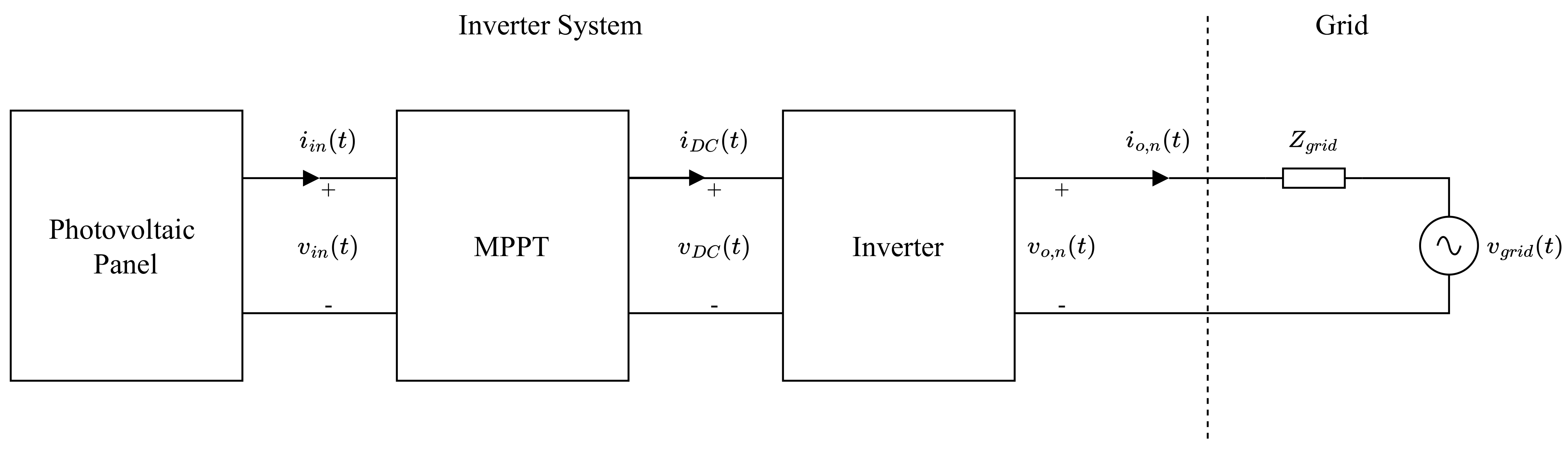
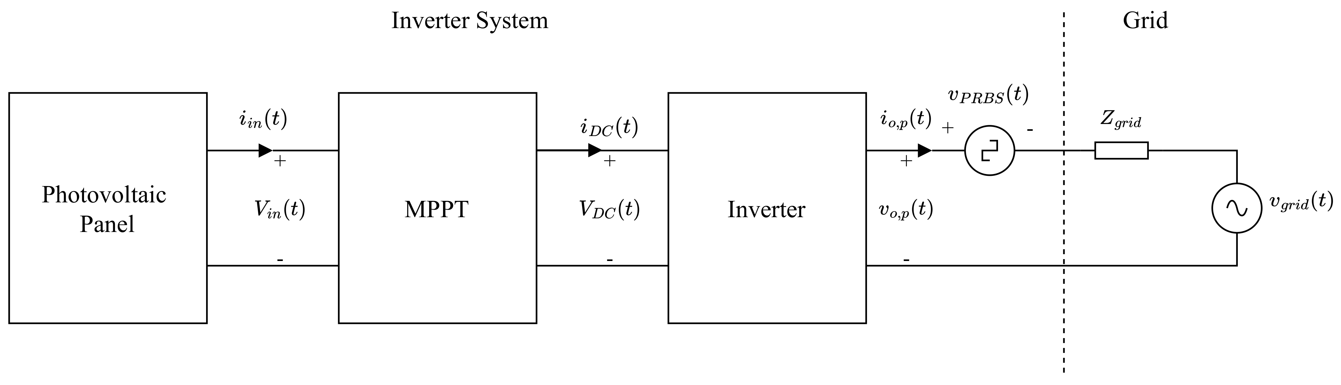
2. Grid-Tied Inverter

2.1. Inverter Topology

Figure 1 shows the circuit configuration of the grid-tied inverter under investigation [60]. The grid is modeled using an AC voltage source in series with a resistor, $R_{grid}$, and inductor, $L_{grid}$. The inverter operates at a fundamental frequency of $f_1=50$ Hz. An LCL filter is used to filter higher-order harmonics produced by the switching circuit. The studied inverter does not employ any method to dampen the resonance that is introduced by the LCL filter. The inductor current, $i_L\left(t\right)$, is controlled by a continuous controller, $G_c\left(s\right)$, while an outer DC voltage loop that is typical of solar inverters is neglected to reduce the complexity of the inverter model. The output of the control loop is scaled by the gain $K_{PWM}=\frac{1}{V_d}$. A full-bridge switching circuit is used.

Figure 2 presents the controller, $G_c\left(s\right)$, that controls the inductor current. $G_c\left(s\right)$ comprises of the sum of two controllers namely a resonant controller, $G_{pr}\left(s\right)$ and a proportional controller, $k_p$.

Equation (1) shows the Laplace-domain representation of the controller $G_{pr}\left(s\right)$.

$$G_{pr}\left(s\right)=\frac{2k_i{\omega }_{pr}s}{s^2+2{\omega }_{pr}s+{w_g}^2}$$

(1)

The filter and controller parameter values of the inverter, as presented by Pastor and Dudrik [60], are listed in

Table 1. Controller and filter parameter values of the grid-tied inverter that is investigated.

Parameter	${\mathit{k}}_{\mathit{p}}$	${\mathit{k}}_{\mathit{i}}$	${\mathit{\omega }}_{\mathbf{pr}}$	${\mathit{\omega }}_{\mathit{g}}$	Cf [$\mathsf{\mu }\mathbf{F}$]	Lf [mH]	Lg [$\mathsf{\mu }\mathbf{H}$]
Value	5.4	400	1	314.16	5.3	18	9

.

2.2. Mathematical Analysis of Inverter

Based on Figure 1, the Laplace-domain representation of the modulation voltage, $v_{Ao}\left(t\right)$, is

$$V_{Ao}\left(s\right)=s{L}_f{I}_L\left(s\right)+s{L}_g{I}_o\left(s\right)+V_o\left(s\right),$$

(2)

where s is the Laplace operator. The inductor current, $I_L\left(s\right)$, is equal to the sum of the capacitor current, $I_C\left(s\right)$, and the output current, $I_o\left(s\right)$,

$$I_L\left(s\right)=I_c\left(s\right)+I_o\left(s\right).$$

(3)

The capacitor voltage, $V_C\left(s\right)$ is described in terms of $I_C\left(s\right)$ as

$$\begin{array}{cc}\hfill V_c\left(s\right)& =\frac{I_c\left(s\right)}{s{C}_f}.\hfill \end{array}$$

(4)

The capacitor voltage, $V_C\left(s\right)$ can be defined in terms of the output voltage as

$$\begin{array}{cc}\hfill V_c\left(s\right)& =s{L}_g{I}_o\left(s\right)+V_o\left(s\right)\hfill \end{array}$$

(5)

Combining (4) and (5) yields

$$\begin{array}{c}\hfill I_c\left(s\right)=s^2{C}_f{L}_g{I}_o\left(s\right)+s{C}_f{V}_o\left(s\right).\end{array}$$

(6)

Using (6) and (3), (2) can be expressed as

$$V_{Ao}\left(s\right)=s{L}_f(s^2{L}_g{C}_f{I}_o\left(s\right)+V_o\left(s\right)s{C}_f+I_o\left(s\right))+s{L}_g{I}_o\left(s\right)+V_o\left(s\right).$$

(7)

The voltage $V_{Ao}\left(s\right)$ is described in terms of the control loop as

$$V_{Ao}\left(s\right)=(k_p+G_{pr}\left(s\right))(I_{ref}\left(s\right)-I_L\left(s\right))$$

(8)

Substituting $I_L\left(s\right)$ using (3) and (6) yields

$$V_{Ao}\left(s\right)=(k_p+G_{pr})I_{ref}\left(s\right)-(k_p+G_{pr})(I_o\left(s\right)+s^2{L}_g{C}_f{I}_o\left(s\right)+V_o\left(s\right)s{C}_f)$$

(9)

Equations (7) and (9) can be combined to obtain

$$\begin{array}{cc}\hfill V_o\left(s\right)(s^2{L}_f{C}_f+1+k_{p}s{C}_f+G_{pr}\left(s\right)s{C}_f)& =I_o\left(s\right)(-k_p-k_p{s}^2{L}_g{C}_f-G_{pr}\left(s\right)-s^2{L}_g{C}_f{G}_{pr}\left(s\right)\hfill \\ \hfill & -s^3{L}_f{L}_g{C}_f-s{L}_f-s{L}_g)+(k_p+G_{pr}\left(s\right))I_{ref}\left(s\right).\hfill \end{array}$$

(10)

The equivalent output impedance of the inverter, $Z_o\left(s\right)$, can be obtained by setting $I_{ref}\left(s\right)=0A$ in (10):

$$Z_o\left(s\right)=\frac{V_o\left(s\right)}{I_o\left(s\right)}{|}_{I_{ref}\left(s\right)=0}$$

(11)

The transfer function of $Z_o\left(s\right)$ has the form:

$$Z_o\left(s\right)=\frac{b_0{s}^5+b_1{s}^4+b_2{s}^3+b_3{s}^2+b_{4}s+b_5}{a_0{s}^5+a_1{s}^4+a_2{s}^3+a_3{s}^2+a_{4}s+a_5}$$

(12)

Table 2. Coefficients of the transfer function of $Z_o\left(s\right)$.

Coefficient	Value
$b_0$	$C_f{L}_f{L}_g$
$b_1$	$C_f{L}_g(k_p+2L_f{\omega }_{pr})$
$b_2$	$L_f+L_g+2C_f{L}_g{k}_i{\omega }_{pr}+2C_f{L}_g{k}_p{\omega }_{pr}+2C_f{L}_g{\omega }_g^2$
$b_3$	$k_p+2L_f{\omega }_{pr}+C_f{L}_g{k}_p{\omega }_g^2$
$b_4$	$2k_i{\omega }_{pr}+L_f{\omega }_g^2+L_g{\omega }_g^2$
$b_5$	$k_p{\omega }_g^2$
$a_0$	0
$a_1$	$C_f{L}_f$
$a_2$	$C_f{k}_p+2C_f{L}_f{\omega }_{pr}$
$a_3$	$1+2C_f{k}_i{\omega }_{pr}+2C_f{k}_p{\omega }_{pr}+C_f{L}_f{\omega }_g^2$
$a_4$	$2{\omega }_{pr}+C_f{k}_p{\omega }_g^2$
$a_5$	${\omega }_g^2$

lists the coefficients of the output impedance, $Z_o\left(f\right)$, in (12). It can be seen from (12) and Table 2 that the inverter impedance is a function of the filter and controller parameters. Therefore, the output impedance is suitable to use in the estimation of inverter filter and controller parameters.

The analytical transfer function presented in (12) is populated with parameters from Table 1 and is used to obtain the frequency response of $Z_o\left(f\right)$ which is presented in Figure 3. It can be seen from Figure 3 that multiple resonant points exist in the output impedance due to the interaction of the LCL filter and the control loop. The impedance $Z_o\left(f\right)$ is almost resistive at 10 Hz. Two parallel resonant points are evident at approximately 50 Hz and 515 Hz. The resonance at 50 Hz can be attributed to the proportional and resonant controller, whereas that at 515 Hz is attributed to the interaction of the filter inductor, $L_f$, and filter capacitor, $C_f$. A series resonant point can also be observed at approximately 23 kHz and is attributed to the LCL elements $L_g$ and $C_f$.

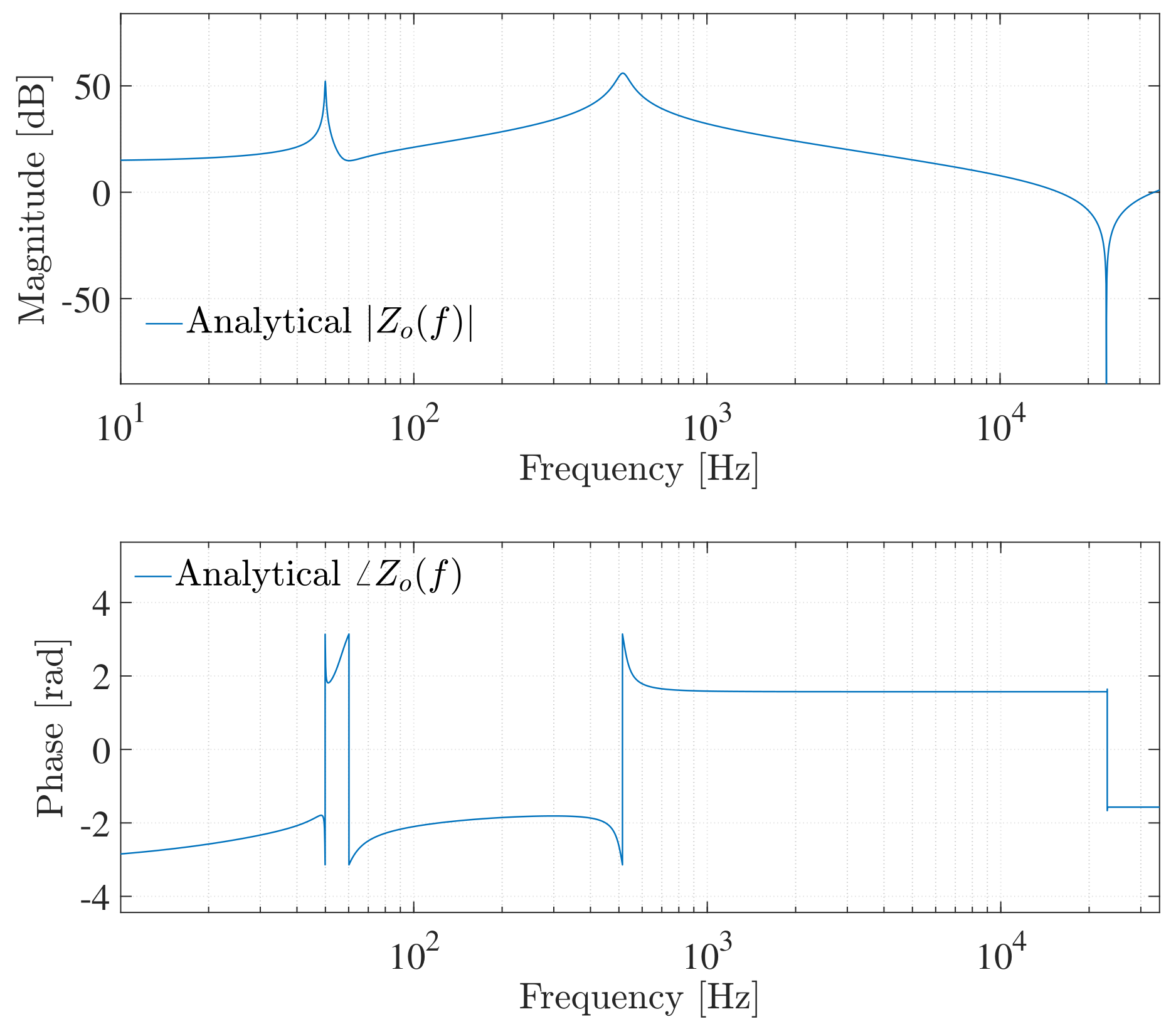
3. Simulated Small-Signal Analysis of Inverter

In this section, the output impedance of the grid-tied inverter described in Section 2.1 is estimated through simulation. The simulation is conducted using the PLECS blockset in Simulink. The inverter model is populated with filter and controller parameters indicated in Table 1. A PRIS perturbation source is connected at the AC output side of the inverter, in parallel with the grid, to produce small-signal perturbations. Figure 4 presents the perturbation arrangement. The PRIS source is constructed using a PRBS14 and a clock frequency, $f_{clk}=2.5$ kHz. The PRIS time constants are chosen as ${\tau }_1=0.1\times T_{clk}$ and ${\tau }_2=10\times T_{clk}$ [21].

The inverter presented in Figure 1 is simulated under normal operating conditions, without perturbation, as well as perturbed conditions, as presented in Figure 4. Voltage and current waveforms from the normal and perturbed state are recorded over a time interval. Equation (13) is subsequently used to extract the inverter output frequency response.

$$Z_o\left(f\right)=\frac{V_{o,p}\left(f\right)-V_{o,n}\left(f\right)}{I_{o,p}\left(f\right)-I_{o,n}\left(f\right)},$$

(13)

where $V_{o,n}\left(f\right)$ and $I_{o,n}\left(f\right)$ indicate the frequency-domain output voltage and current during the normal operation, whereas $V_{o,p}\left(f\right)$ and $I_{o,p}\left(f\right)$ indicate the frequency-domain output voltage and current during perturbation.

Figure 5 compares the estimated output impedance frequency response obtained through simulation with the analytical output impedance frequency response. The estimated $Z_o\left(f\right)$ obtained through simulation agrees well with the analytical $Z_o\left(f\right)$, as the responses lie on top of each other. It should be noted that the RLC circuit of the PRIS perturbation source does not influence the general shape of the impedance frequency response of the system under test but only the time- and frequency-domain characteristics of the perturbation signal. The role of the RLC circuit is to block the fundamental frequency voltages and currents induced by the grid using the series capacitor. Furthermore, the RLC circuit enhances the controllability of the perturbation signal [21].

4. Parameter Estimation

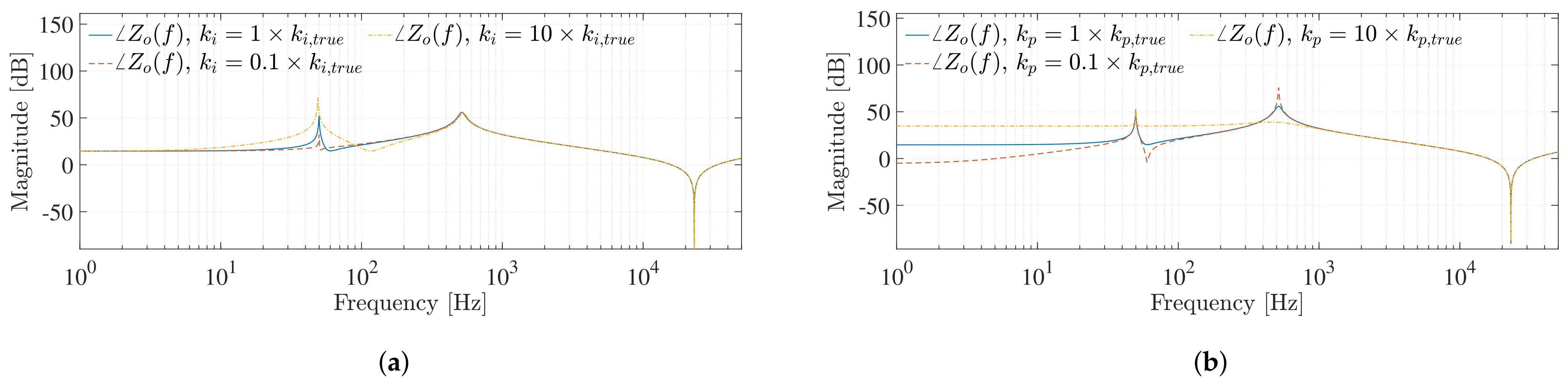
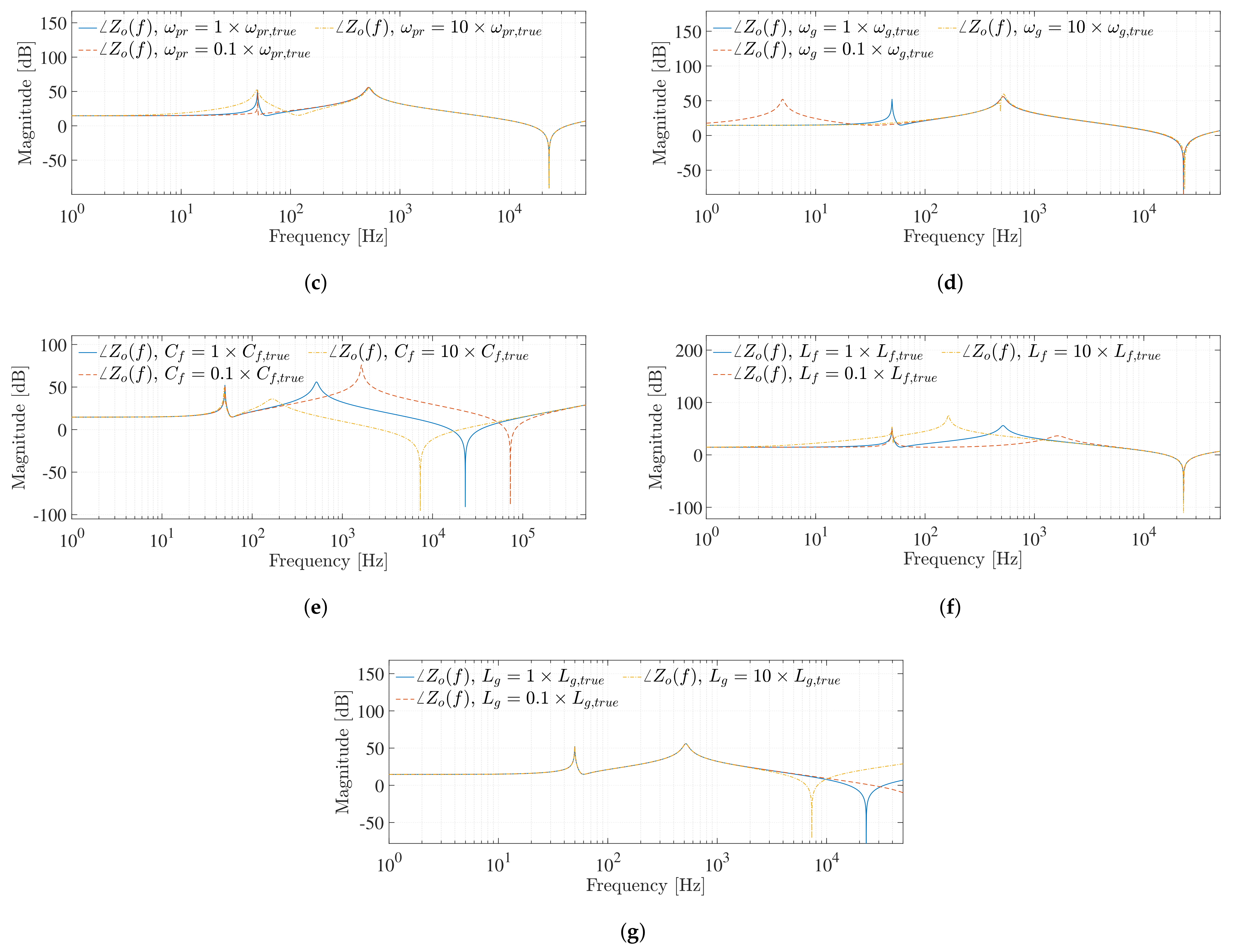
4.1. Frequency-Domain Sensitivity Analysis of Filter and Controller Parameters

Prior to conducting a parameter estimation study, a sensitivity analysis is performed on the analytical output impedance frequency response to determine the influence of the inverter controller and filter parameters on the frequency response. Each filter and controller parameter is varied $10\times$ higher and lower than its true value, while the remaining parameters are fixed. The resultant output impedance frequency responses are compared. Figure 6 shows the output impedance as a function of the filter and controller parameters.

From Figure 6 it can be seen that the inverter controller and filter parameters have an effect on the output impedance frequency response. Depending on the parameter, the effect can be a damping or shifting of the resonant points or a combination thereof. It can be seen that the controller parameters have a greater effect on $Z_o\left(f\right)$ at lower frequencies, including damping of the first parallel resonance. Figure 6e,f show that the second parallel resonance can be attributed to filter capacitor $C_f$ resonating with filter inductor $L_f$. The series resonance can be attributed to filter capacitor $C_f$ resonating with filter inductor $L_g$. Using the output impedance during parameter estimation is thus viable, as all parameters influence its frequency response.

Table 3. Summary of the effect of the controller and filter parameters on the resonant frequency points of the output impedance.

	50 Hz		58 Hz		515 Hz		23 kHz
Parameter	Damping	Shifting	Damping	Shifting	Damping	Shifting	Damping	Shifting
$k_i$	x			x
$k_p$			x		x
${\omega }_{pr}$	x			x
${\omega }_g$	x	x
$C_f$					x	x		x
$L_f$					x	x
$L_g$							x	x

summarizes the effects of the filter and controller parameters on the resonant points of the output impedance frequency response.

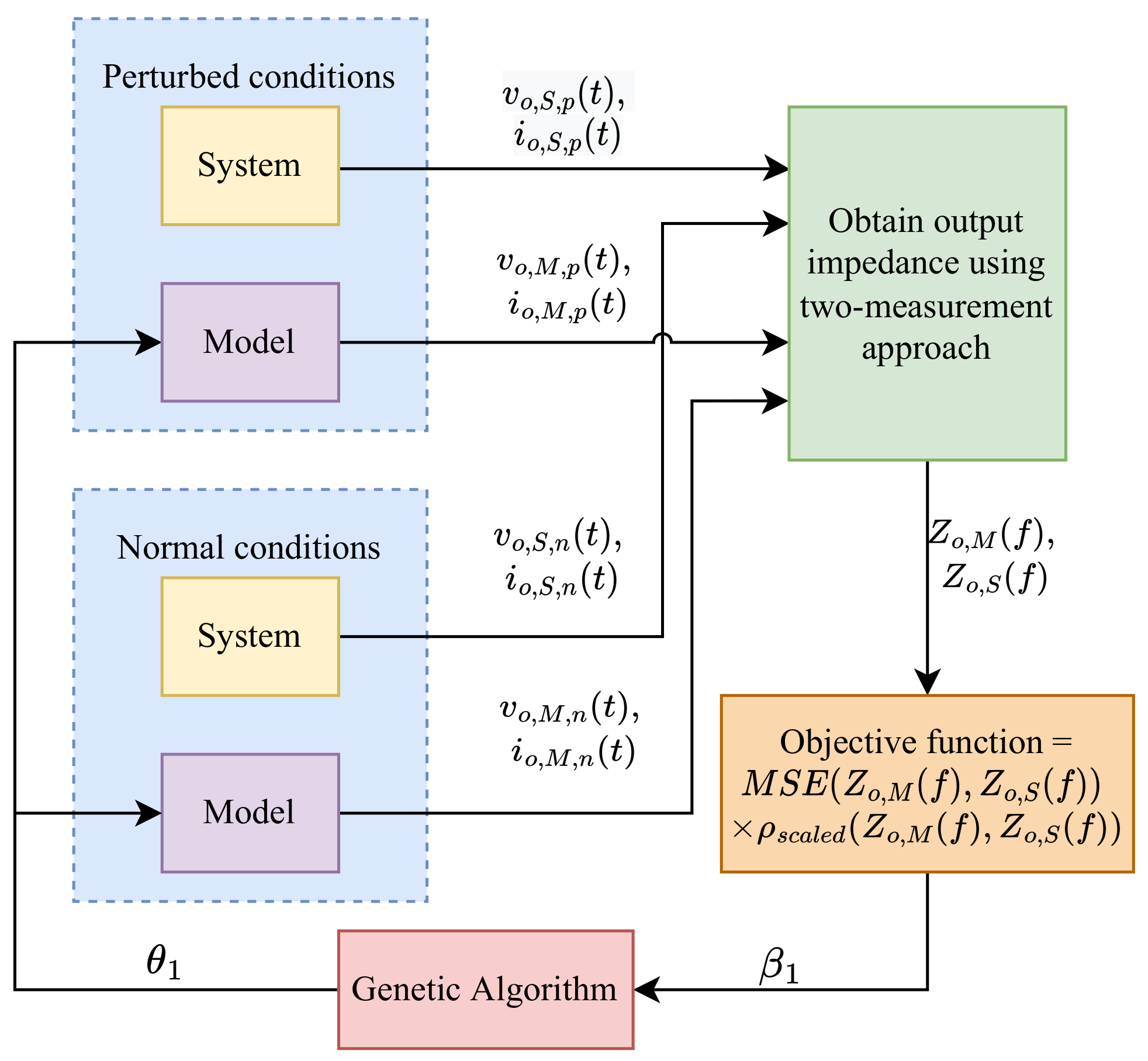
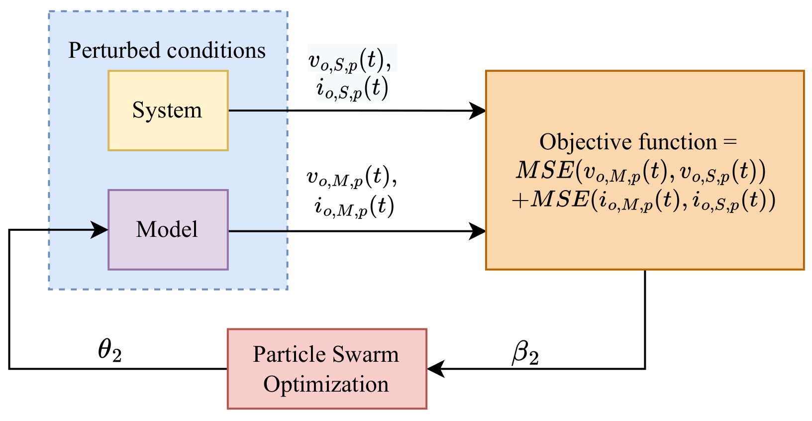
4.2. Parameter Estimation Methodology

The aim of a parameter estimation study is to determine a model’s accurate parameter values from data measured on a target system. In this section, a parameter estimation methodology aimed at obtaining accurate inverter controller and filter parameter values is demonstrated through simulation. The target system, denoted with the subscript “S,” is a simulation of the inverter shown in Figure 1 with the parameters fixed to the values listed in Table 1. An inverter model, denoted with the subscript “M” and whose parameter values are unknown, will be estimated by comparing the time- and frequency-domain outputs of the model and the system. The model parameter values are iteratively tuned using a suitable optimization algorithm in order to minimize the error between the compared model and system outputs. The model and system are operated under normal operating conditions, denoted with the subscript “n,” and perturbed conditions, denoted by the subscript “p.”

The filter and controller parameters that will be estimated are denoted by the vector $\theta$,

$$\theta =[k_p,k_i,{\omega }_{pr},{\omega }_g,C_f,L_f,L_g]$$

(14)

To estimate $\theta$, a two-step parameter estimation process is adopted. Figure 7 demonstrates the parameter estimation methodology used during the first step of the parameter estimation process. In the first step of the parameter estimation process, the lower and upper bounds are chosen as $\theta /10$ and $10\times \theta$, respectively. The model and system are operated under both normal and perturbed conditions to obtain the output impedances of the model and system, $Z_{o,M}\left(f\right)$ and $Z_{o,S}\left(f\right)$, as discussed in Section 3. The Genetic Algorithm (GA) is utilized in the first step to minimize an objective function between the Mean Squared Error (MSE) of the measured output impedance of the model, $Z_{o,M}\left(f\right)$ and the estimated system output impedance, $Z_{o,S}\left(f\right)$, multiplied with the scaled correlation coefficient, ${\rho }_{scaled}$, defined as [31]

$${\rho }_{scaled}(Z_{o,M}\left(f\right),Z_{o,S}\left(f\right))=-\rho (Z_{o,M}\left(f\right),Z_{o,S}\left(f\right))+1.$$

(15)

where,

$$\rho (Z_{o,M}\left(f\right),Z_{o,S}\left(f\right))=\frac{1}{N-1}\sum _{n=1}^N\left(\frac{Z_{o,M}\left(f_n\right)-{\mu }_{o,M}}{{\sigma }_{o,M}}\right)\left(\frac{Z_{o,S}\left(f_n\right)-{\mu }_{o,S}}{{\sigma }_{o,S}}\right)$$

(16)

The frequency responses $Z_{o,M}\left(f\right)$ and $Z_{o,S}\left(f\right)$ are of length N. The parameters ${\mu }_{o,M}$ and ${\mu }_{o,S}$ represent the mean of the output impedance frequency response of the model and the system, respectively, while ${\sigma }_{o,M}$ and ${\sigma }_{o,S}$ indicate the standard deviations of the output impedance frequency response of the model and the system respectively. The optimization algorithm iteratively updates the model parameters, ${\theta }_1$, to minimize the objective function value, ${\beta }_1$. Random initial starting points are used within the lower and upper bounds of the search space during step 1.

Table 4. Parameters used in the genetic algorithm.

GA Parameters	Parameter Value
Population size	70
Number of real variables	7
Crossover fraction	0.8
Mutation fraction	0.01
Migration fraction	0.2
Seed for random number generator	0
Maximum iterations	700
Population size	200
Parallel computing enabled	Yes

presents the parameters used to populate the genetic algorithm during step 1. These include the initialization parameters, as well as the crossover, mutation, and migration parameters.

Figure 8 illustrates the parameter estimation methodology used during step 2. In the second step, a particle swarm optimization algorithm is used to minimize the objective function consisting of the sum of the MSE between the perturbed output voltage of the model, $v_{o,M,p}\left(t\right)$, and the system, $v_{o,S,p}\left(t\right)$, and the MSE between the perturbed output current of the model, $i_{o,M,p}\left(t\right)$, and system, $i_{o,S,p}\left(t\right)$. The estimated parameters after the first step, ${\theta }_1$, are used to reduce the lower and upper bounds for the second step to $0.5\times {\theta }_1$ and $2\times {\theta }_1$, respectively. The system and model are operated under perturbed conditions. The output current and voltage of the system during perturbed operation, $i_{o,S,p}\left(t\right)$, $v_{o,S,p}\left(t\right)$, as well as that of the model during perturbed operation, $i_{o,M,p}\left(t\right)$, $v_{o,M,p}\left(t\right)$, are used in the objective function. The optimization algorithm minimizes the objective function value, ${\beta }_2$, by iteratively updating the model parameters, ${\theta }_2$. Random initial starting points are used within the lower and upper bounds of the search space during step 2.

Table 5. Parameters used in the particle swarm optimization algorithm.

Particle Swarm Parameters	Parameter Value
Maximum inertia weight	0.1
Minimum inertia weight	1.1
Maximum iterations	1400
Minimum adaptive neighborhood size	0.25
Particle velocity adjustment weight	1.49
Neighbourhood velocity adjustment weight	1.49
Swarm size	100

presents the parameters used to populate the particle swarm optimization algorithm during step 2. These include the inertia weights and velocities of both the particles, as well as the neighborhoods.

The particle swarm optimization algorithm and genetic algorithm are global solvers. A multitude of global solvers exists and could have been used to determine the global minimum. The genetic algorithm is generally time-consuming as it arrives at the global minimum by brute force. In comparison to the genetic algorithm, the particle swarm optimization algorithm generally requires fewer function evaluations to arrive at the global minimum. By trying various global optimization algorithms, it is observed that these solvers work best in this specific application.

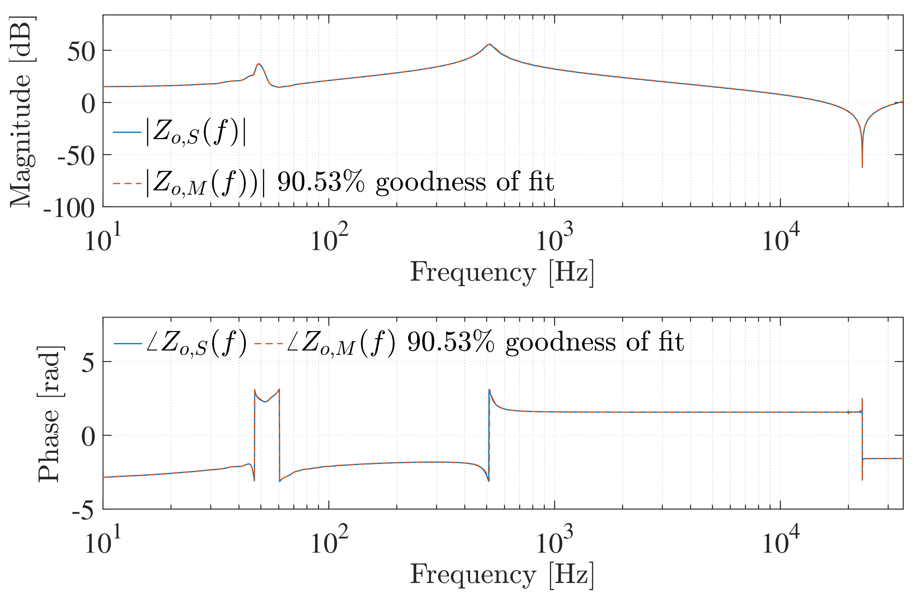
4.3. Parameter Estimation Results

Table 6. Parameter estimation results of the grid-tied inverter.

Step	${\mathit{k}}_{\mathit{p}}$	kp Error [%]	${\mathit{k}}_{\mathit{i}}$	ki Error [%]	${\mathit{\omega }}_{\mathbf{pr}}$	ωpr Error [%]	${\mathit{\omega }}_{\mathit{g}}$	ωg Error [%]	Cf [$\mathsf{\mu }$F]	Cf Error [%]	Lf [mH]	Lf Error [%]	Lg [$\mathsf{\mu }$H]	Lg Error [%]
1	4.76	11.89	560.60	40.15	0.60	40.29	313.35	0.26	6.27	18.27	15.20	15.54	7.61	15.44
2	5.40	0.02	400.08	0.02	0.99	0.03	314.16	0.00	5.3	0.02	0.018	0.01	9	0.05

presents the estimated parameters after step 1, ${\theta }_1$, and step 2, ${\theta }_2$. Although the parameters are not accurately estimated after the first step, the bounds can be significantly reduced for the second step. The estimated parameters after the second step are all estimated within $0.05\%$ accuracy.

Figure 9 shows the output impedance frequency response of the estimated model, $Z_{o,M}\left(f\right)$, compared to the output impedance frequency response of the target system, $Z_{o,S}\left(f\right)$. The estimated output impedance of the model is a good estimation of the target system, as the frequency responses lie on top of each other. This indicates the ability of the proposed methodology to estimate the inverter controller and filter parameters.

5. Experimental Comparison of Pseudo-Random Perturbation

In order to verify the correctness of the proposed inverter impedance characterization methodology, two pseudo-random perturbations, the PRBS and PRIS, are used separately to excite a practical inverter. The experimental perturbation of a practical inverter using a PRBS excitation source is then compared to that of a PRIS excitation source.

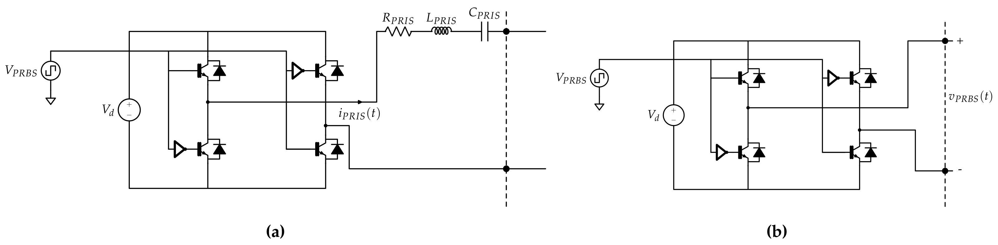
5.1. Pseudo-Random Perturbation Sources

Figure 10a,b present the circuit configuration of a PRIS source [21] and a PRBS source, respectively. Both configurations are constructed using an H-bridge supplied with a DC voltage source, $V_d$. A PRBS gating signal is used to control the switching of the H-bridge circuit for both the PRIS and PRBS sources. The PRIS source additionally includes a series RLC circuit that is connected between the H-bridge and the device under test. This allows for increased control of the spectral characteristics of the perturbation source [21]. In addition, the capacitor, $C_{PRIS}$, protects the switches by limiting the voltage across the PRIS source.

Figure 11 presents the source that is used as both the PRIS source and the PRBS source by including or excluding the RLC filter to obtain the experimental results. The source can withstand a voltage of 1.6kV at the point of connection and a maximum current of 25 A.

The Data Acquisition (DAQ) system used is the 8-Slot NI cDAQ-9178 chassis together with a 16-bit, 4-channel voltage input module, the NI 9223, with a sampling frequency of 1 MHz. A high-voltage differential PINTECH N1000A probe, as well as a GWINSTEK GCP-1000 current probe, is used during the experimental measurements.

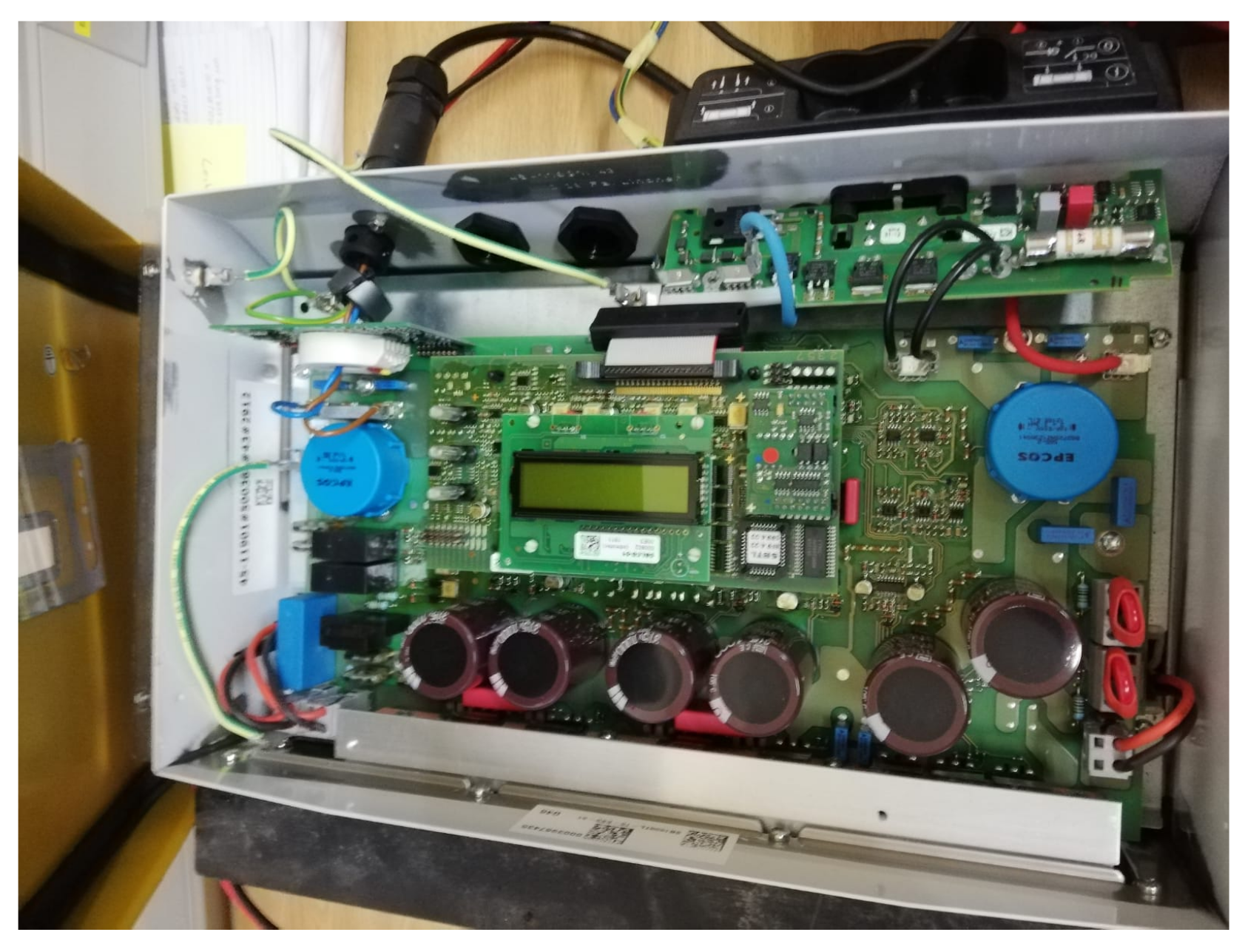
5.2. Description of the Practical Inverter under Investigation

In this section, a $1.6$ kW Sunny Boy grid-tied single-phase commercial inverter is investigated.

Table 7. Specifications for the Sunny Boy 1600TL [61].

Specification	Value
Maximum DC Voltage	600V
Nominal DC voltage	400 V
Minimum DC voltage	125 V
Nominal AC power	1600 W
Nominal AC voltage	$220,230,240V_{RMS}$
Maximum output current	$11A_{RMS}$
Power factor	1
Maximum efficiency	$96.0\%$
Topology	Transformerless

summarizes the inverter’s specifications. The inverter has a fundamental frequency of $f_1=50$ Hz. It is rated for $220V_{RMS}$ to $240V_{RMS}$ and can supply up to $1.6$ kW. The inverter can be supplied with a DC input voltage between 125 V and 600 V. It is controlled to supply power at unity power factor with an efficiency of $96\%$.

Figure 12 shows a block diagram of the inverter system under investigation. The inverter is supplied with an array of photovoltaic panels and uses a Maximum Power Point Tracker (MPPT) in a two-stage transformerless inverter topology [62]. The DC input voltage from the photovoltaic panels, $v_{in}\left(t\right)$, is controlled and stepped up or down to produce a constant voltage, $v_{DC}\left(t\right)$, at the input of the inverter. The inverter converts the DC power to AC power. The grid-tied inverter has an inner current control loop and utilizes a Phase Locked Loop (PLL) to synchronize with the grid voltage [6]. The inverter under investigation is modeled as a black box, as no prior information regarding the control-loop design, filter topology, or parameter values exists [41]. The grid is modeled with an AC voltage source in series with the grid impedance, $Z_{grid}$.

The output current and voltage while the inverter is operating under normal conditions, $i_{o,n}\left(t\right)$ and $v_{o,n}\left(t\right)$, are presented in Figure 13. The RMS values of $i_{o,n}\left(t\right)$ and $v_{o,n}\left(t\right)$ are $1.65A_{RMS}$ and $223.84V_{RMS}$ respectively. The inverter is, thus, only operating at 15% of its maximum output current. It is seen from Figure 13 that the current $i_{o,n}\left(t\right)$ contains a large number of harmonics. The harmonic distortion is caused by the inverter’s switching, as the frequency of the current ripple was observed to be the same as that of the switching frequency of the inverter, i.e., $f_{sw}=16$ kHz. The inverter that is investigated in this section is shown in Figure 14.

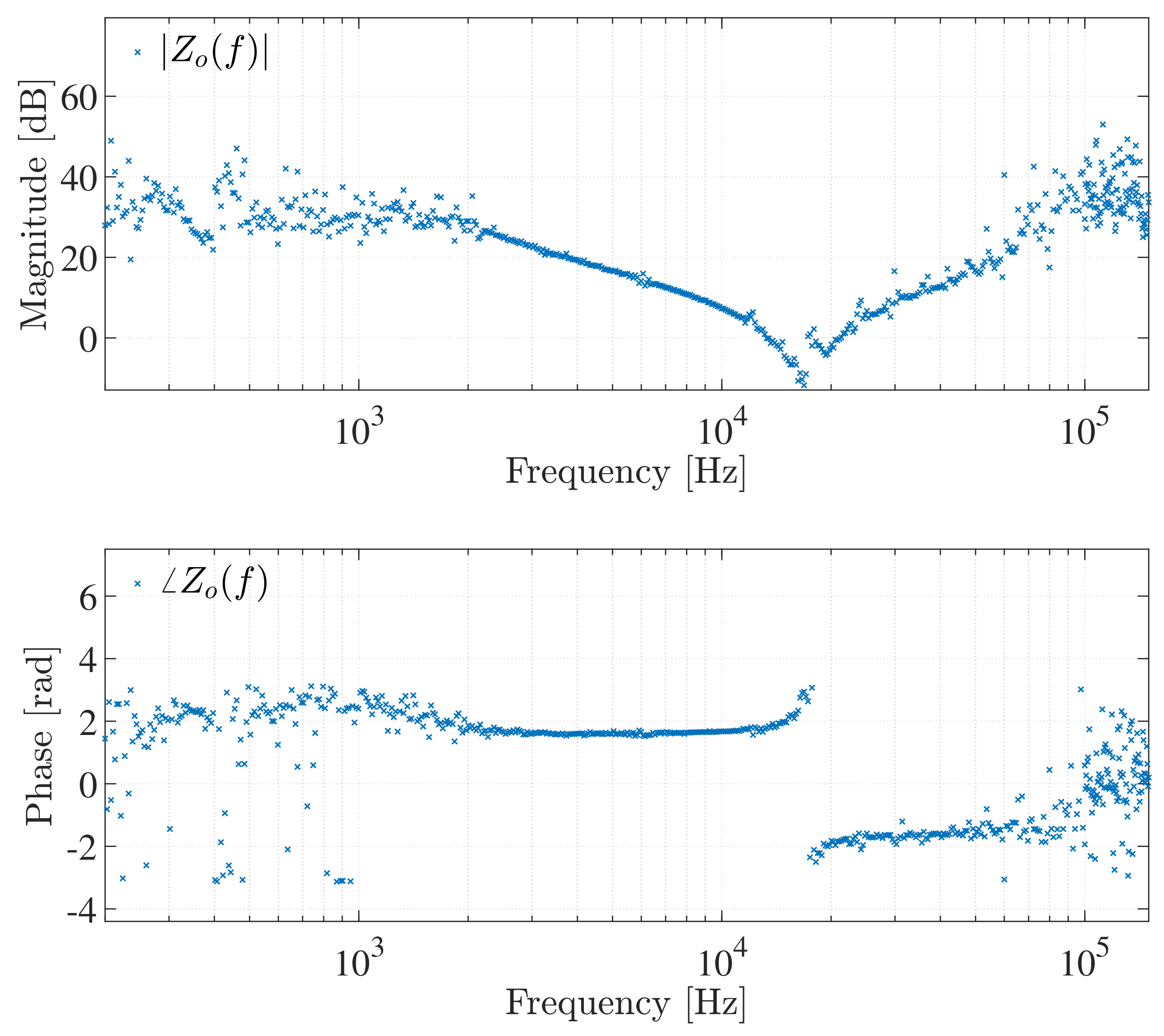
5.3. PRIS Perturbation

The inverter is first perturbed using a PRIS perturbation source. A PRIS source is connected in parallel to the grid. Figure 15 shows a block diagram of the perturbation arrangement where the PRIS source is represented by a current source. The PRIS perturbation source cannot be connected in series between the inverter and the grid, as the impedance of the RLC circuit will distort the grid voltage and prohibit the inverter from connecting to the grid. However, the PRIS source is suitable for connection in parallel, as the RLC is designed to withstand the voltage drop between the H-bridge and the grid voltage. This, however, decreases the perturbation energy of the PRIS source.

To ensure that the inverter is excited across a wide frequency band, two sets of measurements are conducted using a PRIS source. In the first test, a clock frequency of 30 kHz is selected to provide enough perturbation energy in the higher frequency band. Subsequently, a second test is conducted with the clock frequency set to 6 kHz to provide sufficient energy in the lower frequency band. The order, m, of the PRBS gating signal, along with the clock frequency, $f_{clk}$, determines the period, $t_{PRBS}$, of the PRIS, which can be expressed as:

$$t_{PRBS}=\frac{2^m-1}{f_{clk}}$$

(17)

The PRBS order is chosen to keep $t_{PRBS}\approx 1$ s, based on the value of $f_{clk}$. The magnitude of the DC voltage of the perturbation source, $V_d$, is chosen as high as possible but within the limits of the voltage, current, and power ratings of the RLC filter components. The RLC values are selected such that suitable time constants, that ensure sufficient perturbation in the frequency band of interest, are achieved [21].

Table 8. Parameters for two different arrangements of the PRIS source, setup 1 and setup 2.

Setup	PRBS Order	${\mathit{f}}_{\mathit{clk}}$	${\mathit{V}}_{\mathit{d}}$	${\mathit{R}}_{\mathit{PRIS}}$	${\mathit{L}}_{\mathit{PRIS}}$	${\mathit{C}}_{\mathit{PRIS}}$
1	15	30 kHz	160 $V_{DC}$	100 $\mathrm{\Omega }$	2.2 mH	100 nF
2	12	6 kHz	160 $V_{DC}$	100 $\mathrm{\Omega }$	1 mH	1 $\mathsf{\mu }$F

summarize the values of the parameters used to configure the PRIS source.

Figure 16 shows the small-signal perturbations obtained after PRIS perturbation is applied to the inverter using setup 2. The normal, $i_{o,n}\left(t\right)$ and $v_{o,n}\left(t\right)$, and perturbed, $i_{o,p}\left(t\right)$ and $v_{o,p}\left(t\right)$, current and voltage measurements are subtracted to obtain the small-signal perturbations. Both the small-signal current and voltage perturbations have impulse characteristics.

The measured output impedance of the inverter, $Z_o\left(f\right)$, is subsequently determined using the small-signal perturbations and (13). The output impedance is obtained for both sets of measurements, and concatenated at 100 kHz, as this provided the least variance in the output impedance, based on visual inspection. Figure 17 presents the measured $Z_o\left(f\right)$. A series resonant point is evident at approximately 17 kHz. The measured frequency response of $Z_o\left(f\right)$ at frequencies below 2 kHz is distorted, as well as at frequencies greater than 60 kHz. This can be attributed to insufficient perturbation energy in these frequency regions. The insufficient perturbation of the inverter at lower frequencies below 100 Hz can also be attributed to the inverter’s controller operation aiming to control the fundamental 50 Hz component of the output current. In an attempt to improve the estimation of the output impedance at frequencies lower than 2 kHz, $f_{clk}$ of the PRIS source was decreased but did not improve results. Due to insufficient spectral energy in the low-frequency band below 100 Hz, the frequency response of the inverter is presented from 100 Hz.

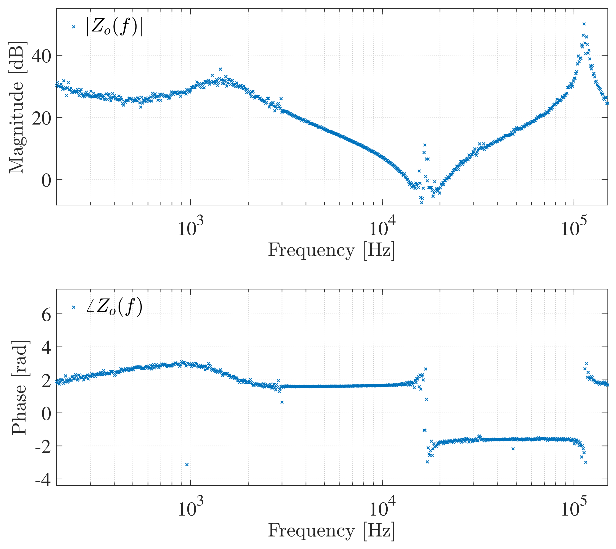
5.4. PRBS Perturbation

A second experiment involving the excitation of the inverter described in Section 5.2 was conducted by using PRBS perturbation. Figure 18 presents a block diagram of the practical arrangement during PRBS perturbations. A PRBS source is connected in series between the AC output side of the inverter and the grid. The PRBS source is presented as a voltage source in Figure 18. The PRBS source would, thus, superimpose PRBS voltage perturbations on the voltage produced by the grid. The PRBS source cannot be connected in parallel to the inverter and the grid, as no passive elements are used to mitigate the voltage difference between the H-bridge and the grid voltage. The series connection of the PRBS source causes the current $i_{o,p}\left(t\right)$ to flow through the IGBTs of the H-bridge, as well as the DC voltage source. These circuit elements, therefore, need to be able to withstand this current.

Similar to PRIS perturbation, two different PRBS source configurations are used to perturb the grid-connected inverter, in order to excite a wide frequency band. The clock frequency and PRBS order are chosen using the same criteria as presented in Section 5.3. To minimize the effect on the inverter’s normal operation, the magnitude of $V_d$ should be chosen to be as small as possible while also providing enough perturbation energy. The voltage $V_d$ is chosen as $5V_{DC}$, as this was the smallest voltage that produced adequate perturbation energy.

Table 9. Parameters for two different arrangements of the PRBS source, setup 1 and setup 2.

Setup	PRBS Order	${\mathit{f}}_{\mathit{clk}}$	${\mathit{V}}_{\mathit{d}}$
1	14	16 kHz	5 $V_{DC}$
2	12	3 kHz	5 $V_{DC}$

summarizes the parameters chosen for the PRBS source configurations.

Figure 19 presents the small-signal current and voltage perturbations produced by the PRBS source using setup 2. Again, the normal, $i_{o,n}\left(t\right)$ and $v_{o,n}\left(t\right)$, and perturbed, $i_{o,p}\left(t\right)$ and $v_{o,p}\left(t\right)$, current and voltage measurements are subtracted to obtain the small-signal perturbations. The voltage has clear PRBS perturbation waveforms.

The measured output impedance of the inverter, obtained using PRBS perturbation, is displayed in Figure 20. The frequency response has less variance compared to the output impedance obtained using PRIS perturbations in Figure 17. The output impedance is estimated for both setups, and concatenated at 3 kHz, based on visual inspection of the variance of the output impedance. A damped series resonant point exists at approximately 500 Hz, and is followed by a parallel resonance at approximately $1.5$ kHz. From $1.5$ kHz, the output impedance is predominantly capacitive until approximately 17 kHz where there is a series resonance. A parallel resonant point is also evident at approximately 114 kHz. An artifact is present at approximately 16 kHz, which is attributed to the switching frequency, $f_{sw}$, of the inverter. Due to insufficient spectral energy in the low-frequency band below 100 Hz, the response is quite noisy in this frequency band and therefore omitted in the frequency response shown in Figure 20.

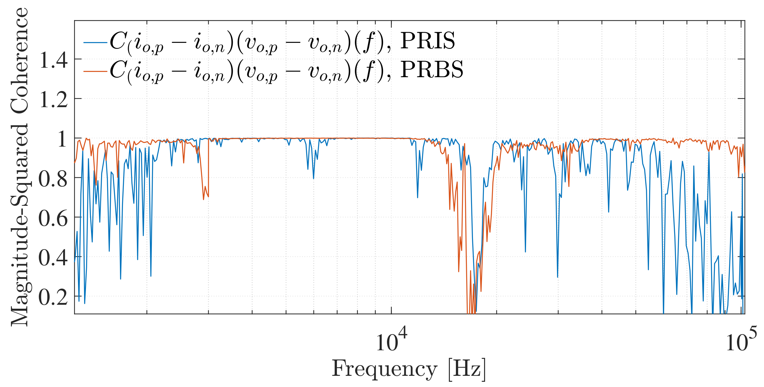
5.5. Critical Comparison of Pseudo-Random Perturbation Strategies

To compare the effectiveness of the PRIS and PRBS perturbation methodologies, the magnitude-squared coherence, $C_{xy}\left(f\right)$, is utilized. The magnitude-squared coherence, $C_{xy}\left(f\right)$, between an input signal, $x\left(t\right)$, and output signal, $y\left(t\right)$, of a transfer function, varies between 0 and 1 in the frequency-domain [63]. A value of 1 indicates a linear relationship between the input and output signals. The magnitude-squared coherence can be calculated using the Cross Power Spectral Density (CPSD), $P_{xy}\left(f\right)$, and Power Spectral Densities (PSDs) of the input, $P_{xx}\left(f\right)$, and output, $P_{yy}\left(f\right)$, signals [63].

$$C_{xy}\left(f\right)=\frac{|P_{xy}{\left(f\right)|}^2}{P_{xx}\left(f\right)P_{yy}\left(f\right)}$$

(18)

The magnitude-squared coherence can be utilized to determine whether the estimated $Z_o\left(f\right)$ obtained for the inverter system is linear or to what extent $Z_o\left(f\right)$ is linear. Figure 21 shows the magnitude-squared coherence between the small-signal currents and voltages, $C_{(i_{o,p}\left(t\right)-i_{o,n}\left(t\right)),(v_{o,p}\left(t\right)-v_{o,n}\left(t\right))}\left(f\right)$, of the PRIS perturbations and the PRBS perturbations between 1 kHz and 150 kHz. The estimated $Z_o\left(f\right)$ using PRIS perturbation is only approximately linear between $2.7$ kHz and 16 kHz, while the linearity also significantly decreases at approximately 6 kHz and $12.4$ kHz in this region. In comparison, the estimated $Z_o\left(f\right)$ using PRBS perturbation is approximately linear throughout this frequency region, with the exception of the frequency region surrounding the switching frequency at 16 kHz.

Table 10. Comparison of the advantages of the PRIS source and the PRBS source.

PRIS Source	PRBS Source
The series RLC circuit that is incorporated in the PRIS source allows for increased protection of the H-bridge and DC source, while also providing an additional means of controlling the time-and frequency-domain characteristics of the PRIS	Fewer components are used to construct the PRBS source
Can be connected in parallel with the system under test thus Can be used to characterize an inverter and the grid simultaneously	Can be connected in series with the system under test and based on practical measurements that are conducted in this work, it produces better perturbation

lists the advantages of the PRIS and PRBS sources for the use of output impedance characterization of inverters.

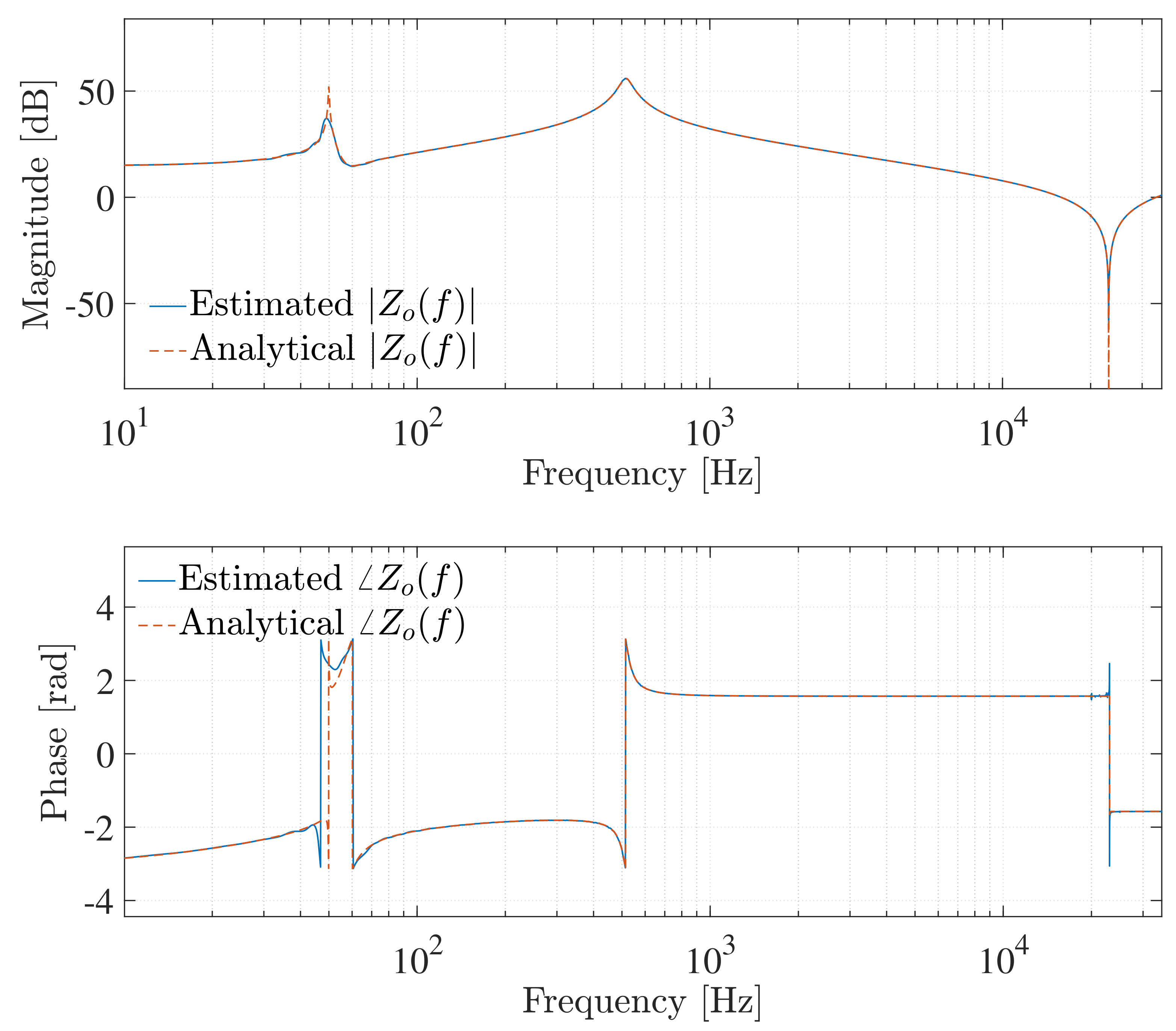
5.6. Estimation of an Analytical Transfer Function of the Inverter Output Impedance from Measurement Data

Due to the lack of access to detailed data on the tested inverter, as is common with most commercial inverters due to manufacturers’ confidentiality, a black-box modeling approach is conducted. In this case, an analytical Laplace-domain transfer function, $Z_{o,approx}\left(s\right)$, that represents the equivalent output impedance of the inverter is approximated from experimental data that was obtained using the PRBS perturbation. The procedure involves selecting the order of the transfer function, whereafter, the Gauss–Newton search is used to determine the coefficients of the transfer function using MATLAB’s tfest function. The instrument variable approach is used for initialization. Up to 5000 iterations are performed, and the initial tolerance is 0.0001. Various orders are investigated, and based on visual observations, a 6^th order transfer function fits the measured $Z_o\left(f\right)$ most accurately. The approximated transfer function of the output impedance, $Z_{o,approx}\left(s\right)$, is:

$$Z_{o,approx}\left(s\right)=\frac{-5.125\times {10}^6{s}^5+8.998\times {10}^{12}{s}^4+2.05\times {10}^{17}{s}^3+1.051\times {10}^{23}{s}^2+7.475\times {10}^{6}26s+1.547\times {10}^{6}30}{s^6-9.276\times {10}^5{s}^5+4.668\times {10}^{11}{s}^4-4.932\times {10}^{17}{s}^3-2.839\times {10}^{6}21s^2-4.213\times {10}^{25}s+7.784\times {10}^{27}}$$

(19)

Figure 22 compares the approximated transfer function, $Z_{o,approx}\left(f\right)$, with the experimental $Z_o\left(f\right)$. The frequency responses lie on top of each other, indicating sufficient accuracy. The estimated transfer function model, $Z_{o,approx}\left(f\right)$, can be used for simulation and inverter power quality studies.

6. Conclusions

In this paper, a methodology for characterizing the output impedance of a single-phase, grid-tied inverter is presented. The methodology involves perturbing, in situ, the AC output side of the inverter with a pseudo-random excitation signal. The obtained output impedance is accurate, as it corresponds well with the analytical output impedance. A parameter estimation study that extracts the controller and filter parameter values from the perturbed inverter measured data is then conducted on the grid-tied inverter. The output impedance, current, and voltage are used to estimate seven filter and controller parameters accurately. Accurate estimation of inverter parameter values can enhance inverter modeling and studies. The parameter estimation methodology suggested and presented in this paper requires prior knowledge of the device under test, such as the inverter’s controller and filter structure. Therefore, this method would allow system designers who have access to this information to accurately model their inverters after experimental testing.

Furthermore, an experimental comparison of pseudo-random perturbation methodologies is investigated. It is shown that the use of PRBS perturbation allows for a more effective characterization of the output impedance of a $1.6$ kW grid-tied inverter compared to a PRIS perturbation. Results, following a black-box modeling approach that involves the estimation of the transfer function of a commercial inverter using experimental data, are also presented. The good agreement between the experimental measurements and the estimated transfer function validates the proposed procedures. Although the system identification methodology that is presented in this paper is case-study specific, the perturbation strategy can be applied to any inverter as long as the pseudo-random perturbation signals can induce persistent excitation for the dynamic modes associated with the target system.

References

1. Rehmani, M.H.; Reisslein, M.; Rachedi, A.; Erol-Kantarci, M.; Radenkovic, M. Integrating Renewable Energy Resources Into the Smart Grid: Recent Developments in Information and Communication Technologies. IEEE Trans. Industr. Inform. 2018, 14, 2814–2825. [Google Scholar] [CrossRef]
2. Tahir, M.; El Shatshat, R.A.; Salama, M. Reactive Power Dispatch of Inverter-Based Renewable Distributed Generation for Optimal Feeder Operation. In Proceedings of the 2018 IEEE Electrical Power and Energy Conference (EPEC), Toronto, ON, Canada, 10–11 October 2018; pp. 1–6. [Google Scholar] [CrossRef]
3. Dileep, D.K.; Bharath, K. A Brief Study of Solar Home Inverters. In Proceedings of the 2018 International Conference on Control, Power, Communication and Computing Technologies (ICCPCCT), Kannur, India, 23–24 March 2018; pp. 334–339. [Google Scholar] [CrossRef]
4. Burkart, R.; Kolar, J.W.; Griepentrog, G. Comprehensive comparative evaluation of single- and multi-stage three-phase power converters for photovoltaic applications. In Proceedings of the International Conference on Telecommunications Energy (INTELEC) 2012, Bengaluru, India, 16–19 December 2012; pp. 1–8. [Google Scholar] [CrossRef]
5. Chowdhury, A.S.K.; Razzak, M.A. Single phase grid-connected photovoltaic inverter for residential application with maximum power point tracking. In Proceedings of the 2013 International Conference on Informatics, Electronics and Vision (ICIEV), Dhaka, Bangladesh, 17–18 May 2013; pp. 1–6. [Google Scholar] [CrossRef]
6. Zhang, Z.; Yang, Y.; Ma, R.; Blaabjerg, F. Zero-Voltage Ride-Through Capability of Single-Phase Grid-Connected Photovoltaic Systems. Appl. Sci. 2017, 7, 315. [Google Scholar] [CrossRef]
7. Ashtiani, N.A.; Ali Khajehoddin, S.; Karimi-Ghartemani, M. Optimal Design of Nested Current and Voltage Loops in Grid-Connected Inverters. In Proceedings of the 2020 IEEE Applied Power Electronics Conference and Exposition (APEC), New Orleans, LA, USA, 15–19 March 2020; pp. 2397–2402. [Google Scholar] [CrossRef]
8. Operator, S. Grid Connection Code for Renewable Power Plants Connected to the Electricity Transmission System or the Distribution System in South Africa; Technical Report; Eskom Transmission Division: Germiston, Johannesburg, South Africa, 2020. [Google Scholar]
9. Rathnayake, H.; Solatialkaran, D.; Zare, F.; Sharma, R. Grid-tied Inverters in Renewable Energy Systems: Harmonic Emission in 2 to 9 kHz Frequency Range. In Proceedings of the 2019 21st European Conference on Power Electronics and Applications (EPE ’19 ECCE Europe), Genova, Italy, 2–6 September 2019; pp. P.1–P.10. [Google Scholar] [CrossRef]
10. Yaghoobi, J.; Zare, F.; Solatialkaran, D. Harmonic Emissions in 0–9 kHz Frequency Range and Transient Effects in Grid-Connected Inverters Utilised in Solar Farms. In Proceedings of the 2020 19th International Conference on Harmonics and Quality of Power (ICHQP), Dubai, United Arab Emirates, 6–7 July 2020; pp. 1–6. [Google Scholar] [CrossRef]
11. Busatto, T.; Ravidran, V.; Larsson, A.; Rönnberg, S.K.; Bollen, M.H.J.; Meyer, J. Experimental Harmonic Analysis of the Impact of LED Lamps on PV Inverters Performance. In Proceedings of the 2019 Electric Power Quality and Supply Reliability Conference (PQ) & 2019 Symposium on Electrical Engineering and Mechatronics (SEEM), Kärdla, Estonia, 12–15 June 2019; pp. 1–4. [Google Scholar] [CrossRef]
12. Langella, R.; Testa, A.; Meyer, J.; Möller, F.; Stiegler, R.; Djokic, S.Z. Experimental-Based Evaluation of PV Inverter Harmonic and Interharmonic Distortion Due to Different Operating Conditions. IEEE Trans. Instrum. Meas. 2016, 65, 2221–2233. [Google Scholar] [CrossRef] [Green Version]
13. Park, J.y.; Nam, S.r.; Park, J.k. Control of a ULTC Considering the Dispatch Schedule of Capacitors in a Distribution System. IEEE Trans. Power Syst. 2007, 22, 755–761. [Google Scholar] [CrossRef]
14. Oue, K.; Sano, S.; Kato, T.; Inoue, K. Stability Analysis of Grid-Forming Inverter in DQ Frequency Domain. In Proceedings of the 2019 20th Workshop on Control and Modeling for Power Electronics (COMPEL), Toronto, ON, Canada, 17–20 June 2019; pp. 1–8. [Google Scholar] [CrossRef]
15. Kato, T.; Inoue, K.; Kawabata, H. Stability analysis of a grid-connected inverter system. In Proceedings of the 2012 IEEE 13th Workshop on Control and Modeling for Power Electronics (COMPEL), Kyoto, Japan, 10–13 June 2012; pp. 1–5. [Google Scholar] [CrossRef]
16. Monshizadeh, P.; De Persis, C.; Stegink, T.; Monshizadeh, N.; van der Schaft, A. Stability and frequency regulation of inverters with capacitive inertia. In Proceedings of the 2017 IEEE 56th Annual Conference on Decision and Control (CDC), Melbourne, Australia, 12–15 December 2017; pp. 5696–5701. [Google Scholar] [CrossRef] [Green Version]
17. Rasheduzzaman, M.; Mueller, J.; Kimball, J. An Accurate Small-Signal Model of Inverter- Dominated Islanded Microgrids Using Reference Frame. IEEE J. Emerg. Sel. Top. Power Electron. 2014, 2, 1. [Google Scholar] [CrossRef]
18. Ebrahimi, M.; Khajehoddin, S.A.; Karimi-Ghartemani, M. Fast and Robust Single-Phase DQ Current Controller for Smart Inverter Applications. IEEE Trans. Power Electron. 2016, 31, 3968–3976. [Google Scholar] [CrossRef]
19. Khalili Senobari, R.; Sadeh, J.; Borsi, H. Frequency response analysis (FRA) of transformers as a tool for fault detection and location: A review. Electr. Power Syst. Res. 2018, 155, 172–183. [Google Scholar] [CrossRef]
20. Roinila, T.; Messo, T.; Luhtala, R.; Scharrenberg, R.; de Jong, E.C.W.; Fabian, A.; Sun, Y. Hardware-in-the-Loop Methods for Real-Time Frequency-Response Measurements of on-Board Power Distribution Systems. IEEE Trans. Ind. Electron. 2019, 66, 5769–5777. [Google Scholar] [CrossRef]
21. Mwaniki, F.; Vermeulen, H. Characterization and Application of a Pseudo-Random Impulse Sequence for Parameter Estimation Applications. IEEE Trans. Instrum. Meas. 2019, 69, 3917–3927. [Google Scholar] [CrossRef]
22. Kim, J.; Kim, H. Length of Pseudorandom Binary Sequence Required to Train Artificial Neural Network Without Overfitting. IEEE Access 2021, 9, 125358–125365. [Google Scholar] [CrossRef]
23. Yan, L.; Bingham, C.; Cruz-Manzo, S.; Cui, D.; Lv, Y. Battery Impedance Measurement Using Pseudo Random Binary Sequences. In Proceedings of the 2020 IEEE 3rd Student Conference on Electrical Machines and Systems (SCEMS), Ji’nan, China, 4–6 December 2020; pp. 686–691. [Google Scholar] [CrossRef]
24. Brozio, C. Modelling of Inverter-Based Generation for Power System Dynamic Studies. IET Gener. Transm. Distr. 2003, 150, 487–492. [Google Scholar] [CrossRef]
25. Roinila, l.T.; Abdollahi, H.; Santi, E. Frequency-Domain Identification Based on Pseudorandom Sequences in Analysis and Control of DC Power Distribution Systems: A Review. IEEE Trans. Power Electron. 2021, 36, 3744–3756. [Google Scholar] [CrossRef]
26. Vermeulen, H.; Strauss, J.; Shikoana, V. On-line estimation of synchronous generator parameters using PRBS perturbations. In Proceedings of the 2003 IEEE Power Engineering Society General Meeting (IEEE Cat. No.03CH37491), Toronto, ON, Canada, 13–17 July 2003; Volume 4, p. 2398. [Google Scholar] [CrossRef]
27. Vermeulen, H.; Strauss, J. Off-line identification of an open-loop automatic voltage regulator using pseudo-random binary sequence perturbations. In Proceedings of the 1999 IEEE Africon. 5th Africon Conference in Africa (Cat. No.99CH36342), Cape Town, South Africa, 28 September–1 October 1999; Volume 2, pp. 799–802. [Google Scholar] [CrossRef]
28. Mwaniki, F.M.; Vermeulen, H.J. Grid Impedance Frequency Response Measurements Using Pseudo-Random Impulse Sequence Perturbation. In Proceedings of the 2019 9th International Conference on Power and Energy Systems (ICPES), Perth, Australia, 10–12 December 2019; pp. 1–6. [Google Scholar] [CrossRef]
29. Mwaniki, F.; Sayyid, A. Characterizing power transformer frequency responses using bipolar pseudo-random current impulses. Int. J. Power Electron. Drive Syst. 2021, 12, 2423. [Google Scholar] [CrossRef]
30. Banks, D.M.; Cornelius Bekker, J.; Vermeulen, H.J. Parameter Estimation of a Two-Section Transformer Winding Model using Pseudo-Random Impulse Sequence Perturbation. In Proceedings of the 2021 56th International Universities Power Engineering Conference (UPEC), Middlesbrough, UK, 31 August–3 September 2021; pp. 1–6. [Google Scholar] [CrossRef]
31. Banks, D.M.; Bekker, J.C.; Vermeulen, H.J. Parameter Estimation of a Three-Section Winding Model using Intrinsic Mode Functions. In Proceedings of the 2022 IEEE International Conference on Environment and Electrical Engineering and 2022 IEEE Industrial and Commercial Power Systems Europe (EEEIC/I&CPS Europe), Prague, Czech Republic, 28 June–1 July 2022; pp. 1–6. [Google Scholar] [CrossRef]
32. Gerber, I.P.; Mwaniki, F.M.; Vermeulen, H.J. Parameter Estimation of a Ferro-Resonance Damping Circuit using Pseudo-Random Impulse Sequence Perturbations. In Proceedings of the 2021 56th International Universities Power Engineering Conference (UPEC), Middlesbrough, UK, 31 August–3 September 2021; pp. 1–6. [Google Scholar] [CrossRef]
33. Solomon, A.; Mwaniki, F.; Vermeulen, H. Application of Pseudo-Random Impulse Perturbation for Characterizing Capacitor Voltage Transformer Frequency Responses. In Proceedings of the 2020 6th IEEE International Energy Conference (ENERGYCon), Gammarth, Tunis, 28 September–1 October 2020; pp. 744–748. [Google Scholar] [CrossRef]
34. Gerber, I.P.; Mwaniki, F.M.; Vermeulen, H.J. Parameter Estimation of a Single-Phase Voltage Source Inverter using Pseudo-Random Impulse Sequence Perturbation. In Proceedings of the 2022 IEEE International Conference on Environment and Electrical Engineering and 2022 IEEE Industrial and Commercial Power Systems Europe (EEEIC/I&CPS Europe), Prague, Czech Republic, 28 June–1 July 2022; pp. 1–6. [Google Scholar] [CrossRef]
35. Wang, Z.; Chai, J.; Xiang, X.; Sun, X.; Lu, H. A Novel Online Parameter Identification Algorithm Designed for Deadbeat Current Control of the Permanent-Magnet Synchronous Motor. IEEE Trans. Ind. Appl. 2022, 58, 2029–2041. [Google Scholar] [CrossRef]
36. Van Rooijen, J.; Vermeulen, H. A perturbation source for in situ parameter estimation applications. In Proceedings of the IECON’94—20th Annual Conference of IEEE Industrial Electronics, Bologna, Italy, 5–9 September 1994; Volume 3, pp. 1819–1823. [Google Scholar] [CrossRef]
37. Yamashita, K.; Renner, H.; Martinez Villanueva, S.; Vennemann, K.; Martins, J.; Aristidou, P.; Van Cutsem, T.; Song, Z.; Lammert, G.; Pabon Ospina, L.; et al. Modelling of Inverter-Based Generation for Power System Dynamic Studies; Joint Working Group C4/C6.35/CIRED; CIGRE: Montreal, QC, Canada, 2018; Volume 298, pp. 81–87. [Google Scholar]
38. Altahir, S.Y.; Yan, X.; Liu, X. A power sharing method for inverters in microgrid based on the virtual power and virtual impedance control. In Proceedings of the 2017 11th IEEE International Conference on Compatibility, Power Electronics and Power Engineering (CPE-POWERENG), Cadiz, Spain, 4–6 April 2017; pp. 151–156. [Google Scholar] [CrossRef]
39. Zhong, Q.C.; Zeng, Y. Can the output impedance of an inverter be designed capacitive? In Proceedings of the IECON 2011—37th Annual Conference of the IEEE Industrial Electronics Society, Melbourne, VIC, Australia, 7–10 November 2011; pp. 1220–1225. [Google Scholar] [CrossRef]
40. Jessen, L.; Fuchs, F.W. Modeling of inverter output impedance for stability analysis in combination with measured grid impedances. In Proceedings of the 2015 IEEE 6th International Symposium on Power Electronics for Distributed Generation Systems (PEDG), Aachen, Germany, 22–25 June 2015; pp. 1–7. [Google Scholar] [CrossRef]
41. Guruwacharya, N.; Bhujel, N.; Tamrakar, U.; Rauniyar, M.; Subedi, S.; Berg, S.E.; Hansen, T.M.; Tonkoski, R. Data-Driven Power Electronic Converter Modeling for Low Inertia Power System Dynamic Studies. In Proceedings of the 2020 IEEE Power & Energy Society General Meeting (PESGM), Virtual Event, 2–6 August 2020; pp. 1–5. [Google Scholar] [CrossRef]
42. Valdivia, V.; Lazaro, A.; Barrado, A.; Zumel, P.; Fernandez, C.; Sanz, M. Black-Box Modeling of Three-Phase Voltage Source Inverters for System-Level Analysis. IEEE Trans. Ind. Electron. 2012, 59, 3648–3662. [Google Scholar] [CrossRef]
43. Reinikka, T.; Roinila, T.; Sun, J. Measurement Device for Inverter Output Impedance Considering the Coupling Over Frequency. In Proceedings of the 2020 IEEE 21st Workshop on Control and Modeling for Power Electronics (COMPEL), Aalborg, Denmark, 9–12 November 2020; pp. 1–7. [Google Scholar] [CrossRef]
44. Gong, H.; Wang, X.; Yang, D. DQ-Frame Impedance Measurement of Three-Phase Converters Using Time-Domain MIMO Parametric Identification. IEEE Trans. Power Electron. 2021, 36, 2131–2142. [Google Scholar] [CrossRef]
45. Wen, B.; Boroyevich, D.; Burgos, R.; Mattavelli, P.; Shen, Z. Small-Signal Stability Analysis of Three-Phase AC Systems in the Presence of Constant Power Loads Based on Measured d-q Frame Impedances. IEEE Trans. Power Electron. 2015, 30, 5952–5963. [Google Scholar] [CrossRef]
46. Liu, J.; Du, X.; Shi, Y.; Tai, H.M. Impedance Measurement of Three-Phase Inverter in the Stationary Frame Using Frequency Response Analyzer. IEEE Trans. Power Electron. 2020, 35, 9390–9401. [Google Scholar] [CrossRef]
47. Jokipii, J.; Messo, T.; Suntio, T. Simple method for measuring output impedance of a three-phase inverter in dq-domain. In Proceedings of the 2014 International Power Electronics Conference (IPEC-Hiroshima 2014—ECCE ASIA), Hiroshima, Japan, 18–24 May 2014; pp. 1466–1470. [Google Scholar] [CrossRef]
48. Li, M.; Nian, H.; Hu, B.; Xu, Y.; Liao, Y.; Yang, J. Design Method of Multi-Sine Signal for Broadband Impedance Measurement Considering Frequency Coupling Characteristic. IEEE J. Emerg. Sel. Top. Power Electron. 2022, 10, 532–543. [Google Scholar] [CrossRef]
49. Li, F.; Wu, J.; Huang, Y.; Zhang, Y.; Zhang, X.; Ma, M. Analysis of online impedance measurement range based on voltage disturbance injection. Energy Rep. 2020, 6, 566–571. [Google Scholar] [CrossRef]
50. Chang, L.; Jiang, X.; Mao, M.; Zhang, H. Parameter Identification of Controller for Photovoltaic Inverter Based on L-M Method. In Proceedings of the 2018 IEEE International Power Electronics and Application Conference and Exposition (PEAC), Shenzhen, China, 4–7 November 2018; pp. 1–6. [Google Scholar] [CrossRef]
51. Zhongqian, L.; Wu, H.; Jin, W.; Xu, B.; Ji, Y.; Wu, M. Two-step method for identifying photovoltaic grid-connected inverter controller parameters based on the adaptive differential evolution algorithm. IET Gener. Transm. Distrib. 2017, 11, 4282–4290. [Google Scholar]
52. Shen, X.; Zheng, J.; Zhu, S.; Shu, L. d-q axis decoupling parameter identification strategy for the grid-connected inverter of photovoltaic generation system. In Proceedings of the 2012 China International Conference on Electricity Distribution, Shanghai, China, 5–6 September 2012; pp. 1–4. [Google Scholar] [CrossRef]
53. Dong, K.; Yan, J.; Shen, W.; Li, S.; Ma, X.; Jia, R. Parameter identification of grid-connected photovoltaic inverter based on adaptive—Improved GPSO algorithm. In Proceedings of the 2019 IEEE 8th International Conference on Advanced Power System Automation and Protection (APAP), Xi’an, China, 21–24 October 2019; pp. 1536–1540. [Google Scholar] [CrossRef]
54. Zhu, H.; Lyu, J.; Xue, T.; Wang, Z.; Dai, J.; Shi, X.; Cai, X. A Controller Parameter Identification Method of PMSG-Based Wind Turbine Generator Based on Measured Impedance. In Proceedings of the 2021 IEEE 12th Energy Conversion Congress & Exposition—Asia (ECCE-Asia), Virtual, 10 October 2021; pp. 1151–1156. [Google Scholar] [CrossRef]
55. Amin, M.; Molinas, M. A Gray-Box Method for Stability and Controller Parameter Estimation in HVDC-Connected Wind Farms Based on Nonparametric Impedance. IEEE Trans. Ind. Electron. 2019, 66, 1872–1882. [Google Scholar] [CrossRef]
56. Zhou, W.; Wang, Y.; Chen, Z. A Gray-Box Parameters Identification Method of Voltage Source Converter Using Vector Fitting Algorithm. In Proceedings of the 2019 10th International Conference on Power Electronics and ECCE Asia (ICPE 2019—ECCE Asia), Busan, Republic of Korea, 27–31 May 2019; pp. 2948–2955. [Google Scholar] [CrossRef]
57. Zhou, W.; Wang, Y.; Cai, P.; Chen, Z. A Gray-Box Impedance Reshaping Method of Grid-Connected Inverter for Resonance Damping. In Proceedings of the 2019 10th International Conference on Power Electronics and ECCE Asia (ICPE 2019—ECCE Asia), Busan, Republic of Korea, 27–31 May 2019; pp. 2660–2667. [Google Scholar] [CrossRef]
58. Zhou, W.; Torres-Olguin, R.E.; Wang, Y.; Chen, Z. A Gray-Box Hierarchical Oscillatory Instability Source Identification Method of Multiple-Inverter-Fed Power Systems. IEEE J. Emerg. Sel. Top. Power Electron. 2021, 9, 3095–3113. [Google Scholar] [CrossRef]
59. Zhou, W.; Torres-Olguin, R.E.; Göthner, F.; Beerten, J.; Zadeh, M.K.; Wang, Y.; Chen, Z. A Robust Circuit and Controller Parameters’ Identification Method of Grid-Connected Voltage-Source Converters Using Vector Fitting Algorithm. IEEE J. Emerg. Sel. Top. Power Electron. 2022, 10, 2748–2763. [Google Scholar] [CrossRef]
60. Pastor, M.; Dudrik, J. Design and control of LCL filter with active damping for grid-connected inverter. In Proceedings of the 2015 International Conference on Electrical Drives and Power Electronics (EDPE), Tatranska Lomnica, Slovakia, 21–23 September 2015; pp. 465–469. [Google Scholar] [CrossRef]
61. SMA. Specification Sheet; Technical Report; SMA Solar Technology AG: Melbourne, Australia, 2010. [Google Scholar]
62. Meneses, D.; Blaabjerg, F.; García, O.; Cobos, J.A. Review and Comparison of Step-Up Transformerless Topologies for Photovoltaic AC-Module Application. IEEE Trans. Power Electron. 2013, 28, 2649–2663. [Google Scholar] [CrossRef] [Green Version]
63. He, J.; Fu, Z.F. 10—Multi-input multi-output modal analysis methods. In Modal Analysis; He, J., Fu, Z.F., Eds.; Butterworth-Heinemann: Oxford, UK, 2001; pp. 198–223. [Google Scholar] [CrossRef]
Figure 1. Circuit diagram of the grid-tied inverter under investigation.
Energies 16 01414 g001
Figure 2. Block diagram of the controller, G c ( s ) .
Energies 16 01414 g002
Figure 3. Magnitude and phase response of the analytical inverter output impedance.
Energies 16 01414 g003
Figure 4. The inverter with the PRIS perturbation source connected at its AC output side.
Energies 16 01414 g004
Figure 5. Magnitude and phase frequency response of the estimated inverter output impedance compared to the analytical inverter output impedance.
Energies 16 01414 g005
Figure 6. The magnitude and phase response of the analytical output impedance, Z o ( f ) , as a function of (a) k i , (b) k p , (c) ω p r , (d) ω g , (e) C f , (f) L f , and (g) L g .
Energies 16 01414 g006aEnergies 16 01414 g006b
Figure 7. Block diagram illustrating the parameter estimation methodology used during step 1.
Energies 16 01414 g007
Figure 8. Block diagram illustrating the parameter estimation methodology used during step 2.
Energies 16 01414 g008
Figure 9. Comparison of the magnitude and phase response of the output impedance of the model after parameter estimation is performed, Z o , M ( f ) , and the target system Z o , S ( f ) .
Energies 16 01414 g009
Figure 10. Circuit configuration of a (a) PRIS source and a (b) PRBS source.
Energies 16 01414 g010
Figure 11. The configurable perturbation source used as both a PRBS and PRIS source.
Energies 16 01414 g011
Figure 12. Block diagram of the inverter system under normal operating conditions.
Energies 16 01414 g012
Figure 13. The output voltage, v o , n ( t ) , and current, i o , n ( t ) , under normal operating conditions.
Energies 16 01414 g013
Figure 14. The inverter under investigation.
Energies 16 01414 g014
Figure 15. Block diagram of the inverter system during PRIS perturbation.
Energies 16 01414 g015
Figure 16. Small-signal perturbations of the current, ( i o , p ( t ) i o , n ( t ) ), and the voltage, ( v o , p ( t ) v o , n ( t ) ), after PRIS perturbation.
Energies 16 01414 g016
Figure 17. Magnitude and phase response of Z o ( f ) of the practical inverter under investigation using PRIS perturbation.
Energies 16 01414 g017
Figure 18. Block diagram of the inverter system during PRBS perturbation.
Energies 16 01414 g018
Figure 19. Small-signal perturbations of the current, ( i o , p ( t ) i o , n ( t ) ), and the voltage, ( v o , p ( t ) v o , n ( t ) ), after PRBS perturbation.
Energies 16 01414 g019
Figure 20. Magnitude and phase response of Z o ( f ) of the practical inverter under investigation using PRBS perturbation.
Energies 16 01414 g020
Figure 21. Magnitude squared coherence, C ( i o , p ( t ) i o , n ( t ) ) , ( v o , p ( t ) v o , n ( t ) ) ( f ) , using PRIS and PRBS perturbations.
Energies 16 01414 g021
Figure 22. Magnitude and phase response of the analytical Laplace-domain approximation of the measured output impedance, Z o , a p p r o x ( f ) , compared to Z o ( f ) .
Energies 16 01414 g022