Article

Optimal Control of a Single-Stage Modular PV-Grid-Driven System Using a Gradient Optimization Algorithm

by
Saleh Masoud Abdallah Altbawi
1,*,
Ahmad Safawi Bin Mokhtar
1,
Saifulnizam Bin Abdul Khalid
1,
Nusrat Husain
2,
Ashraf Yahya
2,
Syed Aqeel Haider
3,
Rayan Hamza Alsisi
4 and
Lubna Moin
2
1
Faculty of Electrical Engineering, Universiti Teknologi Malaysia, Johor Bahru 81310, Johor, Malaysia
2
Department of Electronics & Power Engineering, Pakistan Navy Engineering College, National University of Sciences and Technology (NUST), Islamabad 44000, Pakistan
3
Department of Computer & Information Systems Engineering, Faculty of Electrical & Computer Engineering, NED University of Engineering and Technology, Karachi 75270, Pakistan
4
Department of Electrical Engineering, Faculty of Engineering, Islamic University of Madinah, Madinah 41411, Saudi Arabia
*
Author to whom correspondence should be addressed.
Energies 2023, 16(3), 1492; https://doi.org/10.3390/en16031492
Submission received: 19 December 2022 / Revised: 21 January 2023 / Accepted: 30 January 2023 / Published: 2 February 2023
(This article belongs to the Special Issue Towards Stable Operation and Control of New Energy Power System)

Abstract

:
There are many studies that focus on extracting harmonics from both DC and AC sides of grid-interfaced photovoltaic (PV) systems. Based on these studies, the paper introduces an efficient method depending on hybrid DC voltage, and an active and reactive power (DC-V PQ) control scheme in a single-stage three-phase grid-interfaced PV system. The proposed scheme is designed to regulate DC voltage to minimize power loss and energy share between the network reconfiguration and the utility grid. Moreover, the technique is more effective at dealing with uncertainty and has higher reliability under various operating scenarios. These operations are the insertion of linear load 1, nonlinear load, and linear load 2. Moreover, a novel objective function (OF) is developed to improve the dynamic response of the system. OF is coupled with a particle swarm optimization (PSO) algorithm and a gradient optimization (GBO) algorithm. The analysis and the comparative study prove the superiority of GBO with counterfeits algorithm.

1. Introduction

Single- and two-stage networks are the popular techniques used to design voltage source inverter (VSI)-based PV-grid-connected generators [1]. In the single-stage PV design, the VSC connects to the PV system through regulation of the DC-link voltage, as shown in Figure 1. The dual stage, as illustrated in Figure 2, contains additionally a DC/DC converter connected between the VSI and PV system. In the AC side of both systems, the VSI is cascaded with the utility grid at a point of common coupling through (PCC) after a filter and circuit breaker to secure, manage, and seamlessly transfer power [2].
Single-stage design contains just one energy conversion process, which makes it more convenient, economical, and effective than dual-stage design [3]. As a result of this, many factories and companies tend to adopt single-stage topology in most of their work. To comply with the demand of the industry domain, this paper exclusively focuses on the single-stage PV system [4]. Table 1 gives some brief points between single-stage and dual-stage grid-tied PV systems.
Sustainable development has been hindered by high carbon emissions. In recent years, low-carbon factors have often been incorporated into the objective function or constraints related to carbon emissions or carbon costs. In [5], the authors suggested a novel distributed event-triggered secondary control approach with a design of an autonomous microgrid using a cyber-physical system. However, this method can result in inter-execution times of zero, leading to the accumulation of event times, also known as the Zeno phenomenon, which must be avoided in the design of the controller. One study from the literature [6] proposes a risk-averse, multi-stage method for deploying energy storage in a residential microgrid, taking into account partial operation constraints and uncertainties in renewable energy sources. Although these planning methods consider the multi-stage process of short-term operation, there are no suitable algorithms to solve long-term, hourly, powerful, transmission-constrained unit commitment (TCUC), and economic dispatch (ED) issues. Researchers in [7] developed a carbon-constrained locational marginal price based on carbon emission flow (CEF) to link the prosumer sides in a hierarchical framework. However, it does not address joint E&C trading in distribution networks that would allow consumer participation. In contrast, the generation-based pricing method only imposes a carbon tax on generators, which results in additional costs for consumers and creates an uneven incentive structure. Moreover, these planning methods used in [5,6,7] cannot be applied to solve the planning problem for the main grid with transmission constraints.
Over recent years, many researchers have designed and analyzed control approaches for the voltage source inverter (VSI). A poloidal field power system (PFPS), consisting of grid-interfaced VSIs along with a three-level H-bridge converter, has been introduced in [8] using MPPT control and current control. However, this method does not guarantee optimal power sharing. In [9,10,11] the authors have managed the active and reactive power control in grid-connected microgrids to ensure power sharing while the VSI is not overloaded. However, the power coordinate control strategy does not guarantee an optimal adjustment of the DC link voltage. The scholars in [12] have utilized predictive control (PC) for a single-stage microgrid. However, PC involves a huge number of parameters to define a rejection for the disturbances and they may not recover input fluctuations well. In [13], the researchers have introduced a nonlinear controller using back-stepping and a Lyapunov scheme in a single-stage microgrid. However, this method has limitations as it requires extensive information about the network situations, complex calculations, the generation of a higher amplitude of control signal, and the presence of steady-state error. In [14], dual-stage grid-interfaced photovoltaic systems connected to unbalanced and nonlinear loads have been controlled using a distributing current generator approach. Nonetheless, this approach increases harmonics in transit duration during steady states. D-STATCOM for harmonic minimization using a power balance approach was utilized in [15]. However, this approach causes variation in the DC voltage signal. In [16], the authors performed efficient analysis and control of a grid-connected proton exchange membrane fuel cell (PEMFC) using active and reactive power control. However, there were some limitations in this tactic, such as the air flowing in the opposite direction, which delays the working of the PI controller and decreases the effectiveness throughout the transient control. In [17], optimal voltage regulation in the grid contains three-phase DSTATCOM and the modular multilevel inverter (MMI) along with DC voltage and current control. However, the response of the controller against the changes in the microgrid is slow. A single-stage PV-system-driven utility grid controlled with an order generalized integrator quadrature (ISOGI-Q) in [18], and an improved second-order generalized integrator with frequency-locked loop (ISOGI-FLL) in [19], are used to improve the power quality of the grid. However, both ISOGI-Q and ISOGI-FLL have low performance when they are combined with the DC offset which produces high variation and more harmonics in the frequency. In [20,21,22], the researchers introduced the control of a photovoltaic distribution static compensator (PV-DSTATCOM) interfaced with the utility grid to improve power quality. The control utilizes a least mean fourth (LMF) algorithm, a leaky least mean fourth (LLMF) algorithm, and a leaky least mean logarithmic fourth (LLMLF), respectively. However, all of these algorithms may suffer from the weight drift issue in some situations. In the literature, the authors of [23,24] have used the least mean square (LMS) algorithm, and the variable leaky least mean square (VLLMS) in [25], along with adaptive filters to suppress the harmonic current control strategy. However, these algorithms may suffer deviation because of the lack of spectral excitation or intermittent irradiance in PV. In [26], a combination of multilayer perceptron (MLP) and neural networks to overcome unbalanced situations is demonstrated. However, this combination is time-consuming because every independent variable in the network is affected by all other variables which led to difficulty in the computations.
Scientists tried to improve power quality using different kinds of artificial intelligence, such as reasoning and learning methods with metaheuristics algorithms [27]. In [28], for reasoning and learning methods to estimate the reliability of the control system, the fuzzy critic method was used. Similarly, refs [29,30] utilized fuzzy logic for power quality resilience. However, these methods need a high level of programming and more training tasks.
Nowadays, metaheuristics are more popular due to their advanced level of solutions for different electrical problems. The authors in [31] have utilized the particle swarm (PSO) algorithm, and the hybrid squirrel search algorithm with the whale optimization algorithm (SSAWO) in [32], to improve the dynamic performance of the system, even though PSO and SSAWO suffer from limitations such as slow convergence and a fall in local optima. The researchers have presented real and reactive power control along with a fractional-order PI (FOPI) controller to improve the dynamic performance of fuel cells (FC) for on-grid systems. Then, a modified flower pollination algorithm (MFPA), harmony search (HS), and electromagnetic field optimization (EFO) have been utilized to enhance power quality [33]. However, this control method generates a long steady-state error, while MFPA, HS, and EFO do not guarantee the optimal selection of the FOPI controller’s parameters. In [34], the authors presented the emperor penguin optimizer (EPO) to adjust the initial setting of duty cycle and tune the parameters of the controllers in the PV-grid-driven system. A combination of fuzzy logic and particle swarm optimization (PSO) along with the objective function as mean square error was developed in [35]. This control strategy has achieved advanced performance in controlling off-grid photovoltaic systems.
This paper proposes an effective control strategy to control DC voltage, active power, and reactive power control in grid-connected microgrids. It depends on combining DC control and P/Q control to have a fully supervised system. The classical control methods in grid-connected microgrids face a lot of challenges, such as failure when the nonlinear is connected due to a high level of harmonics and the absence of a DC regulation mechanism. Moreover, the outcome of real and reactive power suffers heavy fluctuations during the transition conditions [36].
In brief, the objectives of the given research are as follows:
-
Introduce an efficient method for the reliable execution of the PV-interfaced utility grid.
-
Regulate active and reactive power and guarantee optimal power sharing.
-
Decrease the fluctuations in real and reactive power which lead to reduced power losses.
-
Fine-tune the DC-link voltage.
-
Improve the transient response significations (percentage overshoot, settling time).
-
Enhance the dynamic response of the proposed method using PSO and GBO.
The paper is organized as follows: Microgrid configuration is presented in Section 2. The optimization procedure is described in Section 3. Results and discussions are provided in Section 4. Finally, we draw conclusions and point to future work in Section 5.

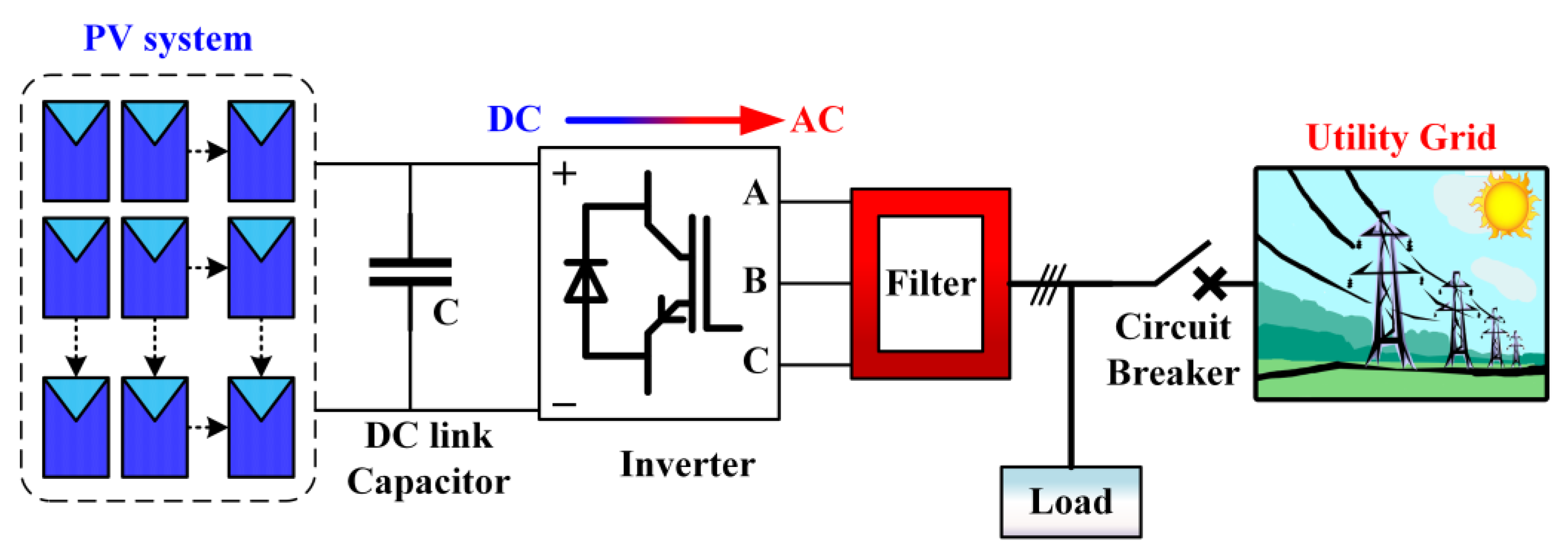
2. Microgrid Configuration

Figure 3 shows the PV network interfaced with a three-phase utility grid consisting of different modules. The photovoltaic modules, LC filter, linear/nonlinear loads, DC-link capacitance, VSI, and the proposed control design are the main components.
In this study, two levels of voltage source inverter (VSI) were used for a three-phase circuit which is symbolized by three legs. In every leg, there are two electronic switches. Depending on the switches’ functions for the desired operation, the required AC voltage from the input DC voltage is required. In addition, the switches have six dynamic cases and two inactive cases. VSI is the most important component in the network, which can integrate control methods to achieve optimal operation in the grid-interfaced microgrid. VSI needs an appropriate control strategy to have an effective damping of the oscillation in real and reactive power output waveforms during different operating scenarios [37].

2.1. Proposed DC Voltage, Active and Reactive Power (DC-V-PQ) Control of Grid-Connected Microgrid

This control method consists of DC voltage control, active–reactive power control, and current control as shown in Figure 4.
Controlling a PV-connected utility grid using a combination of DC voltage control, active power control, and reactive power control on the d axis and q axis has several advantages over controlling the DC voltage only. One of the main advantages is improved power quality. By controlling both the active and reactive power, the system can help to ensure that the grid is being supplied with the correct amount of power while also maintaining a stable voltage level. This can help to prevent voltage fluctuations and power outages, which can occur when the grid is not properly regulated. Moreover, efficiency is also improved. By using a combination of DC voltage control and active/reactive power control, it is possible to achieve a more stable and efficient system. The MPPT algorithm can help to optimize the power output of the PV panels, while the PI controllers can help to adjust the power factor and control the active and reactive power [38].
On the other hand, regulating the DC voltage only can have some limitations. For example, voltage fluctuations may happen due to changes in the temperature and the irradiance of sunlight, which can cause power outages and damage to the devices connected to the utility grid. Moreover, by not controlling the active and nonactive power, the grid may be supplied with an incorrect amount of power, leading to an inefficient system [39].
There are several benefits of using transformations between the ABC, stationary dq0, and rotating alpha-beta-zero (αβ0) reference frames in electrical systems:
(1) These reference frames can simplify the analysis and control of electrical systems and improve their dynamic performance [40]. (2) The dq0 transformation can decouple systems into two independent subsystems, making them easier to analyze and control. (3) The use of these reference frames can help to improve the power quality of electrical systems by isolating and identifying harmonics that can cause problems, such as voltage distortion and increased losses [41].

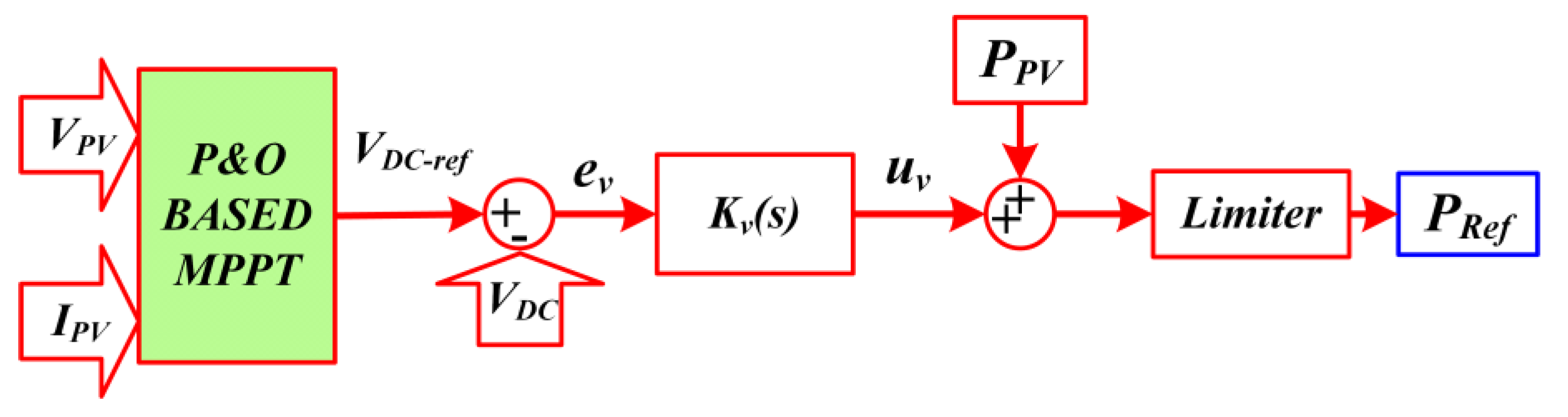
2.2. DC Voltage Control

The proposed control strategy comprises maximum power point tracking (MPPT) and adjusting DC voltage control.

2.2.1. MPPT P&O

The perturb and observe (P&O) procedure is commonly used in MPPT controllers due to its easy implementation and simplicity. The main principle of MPPT P&O depends on the conditions of the voltage and the power [42]. P&O is utilized for MPPT in photovoltaic systems, and functions by making slight adjustments, referred to as “perturbing,” to the operating voltage or current of the PV system, and then observing the resulting change in power output. The process of perturbing involves making small modifications to the voltage or current, while observing refers to measuring the power output after these changes have been made. For instance, if the PV system is currently operating at a specific voltage and current, and the algorithm is investigating whether increasing the voltage will lead to a higher power output, the algorithm will make a small increment to the voltage, and then measure the new power output. If the new power output is greater than the previous output, it suggests that the new voltage is closer to the maximum power point, and the algorithm will continue to raise the voltage. However, if the new power output is less than the previous output, it implies that the new voltage is not at the maximum power point, and the algorithm will decrease the voltage. By repeating this process of perturbing and observing, the algorithm can gradually converge on the maximum power point. Once the maximum power point is reached, the algorithm will keep the system operating at that point to optimize power output [43].
In this case, the algorithm must swap the direction of the perturb voltage to near MPP. After every perturb execution, the existing current I(k) and voltage V(k) are measured, and the power P(k) is calculated. After that, it is compared with the former perturb execution. If the error of voltage e (V) and error of power e (P) are more than zero, then the algorithm keeps the operation in the same direction without change (C = 0). Alternatively, the algorithm works inversely to bring the operating point near MPP, where C is the difference between the current output voltage ( V r e f ( k ) ) and the previous output voltage ( V r e f ( k 1 ) ) [44]. Figure 5 illustrates the conventional MPPT P&O.

2.2.2. Adjusting DC Voltage Control

In this control, the reference DC voltage ( V D C r e f ) is generated by MPPT. This V D C r e f value was compared with the measured DC voltage value to set the DC value near to the nominal DC voltage value. Moreover, this process creates DC error ( V D C e r r ). The V D C e r r is calculated as:
V D C e r r = V D C r e f V D C
where V D C is the measured value of DC volt. Following the control signal, ( D D C ) is produced from the digital PI controller and is added to the active power d axis [45]. It can be given by the following formula:
D D C = V D C e r r × ( K P + K I × ( T s × z z 1 ) )
where T s is the sample time of the error signal and   K P ,   K I are the gains of the PI controller, z indicates the z-conversion of the discrete-time signal of the PI-controller-based closed-loop control system [46].

2.3. Real and Reactive Power References

The output signal of DC voltage control adjusts the real power reference ( P r e f ). This process does not take into account power losses from the voltage source inverter (VSI). The active power, which is roughly equal to the power drawn from the DC side terminals of the VSI, is affected by the difference between the active power at the inverter ( P i n v ) and the incoming PV power ( P P V ). This difference is then integrated by the DC-link capacitor (C), causing the voltage to either increase or decrease. In a steady state, the voltage will settle at the desired level ( V D C r e f ), a result of the integral term of K V ( s ) , and P i n v becomes equal to P P V , which can be expressed as
d d t ( 1 2 C V D C 2 ) P P V P i n v
Figure 6 demonstrates the real power reference generation.
The aim of the nonactive power control is to deliver the desired amount of reactive power to the point of common coupling (PCC), which is defined by the reference value for reactive power ( Q r e f ). In most PV designs, the Q r e f is set to zero in order to maintain a unity power factor with the grid [47].

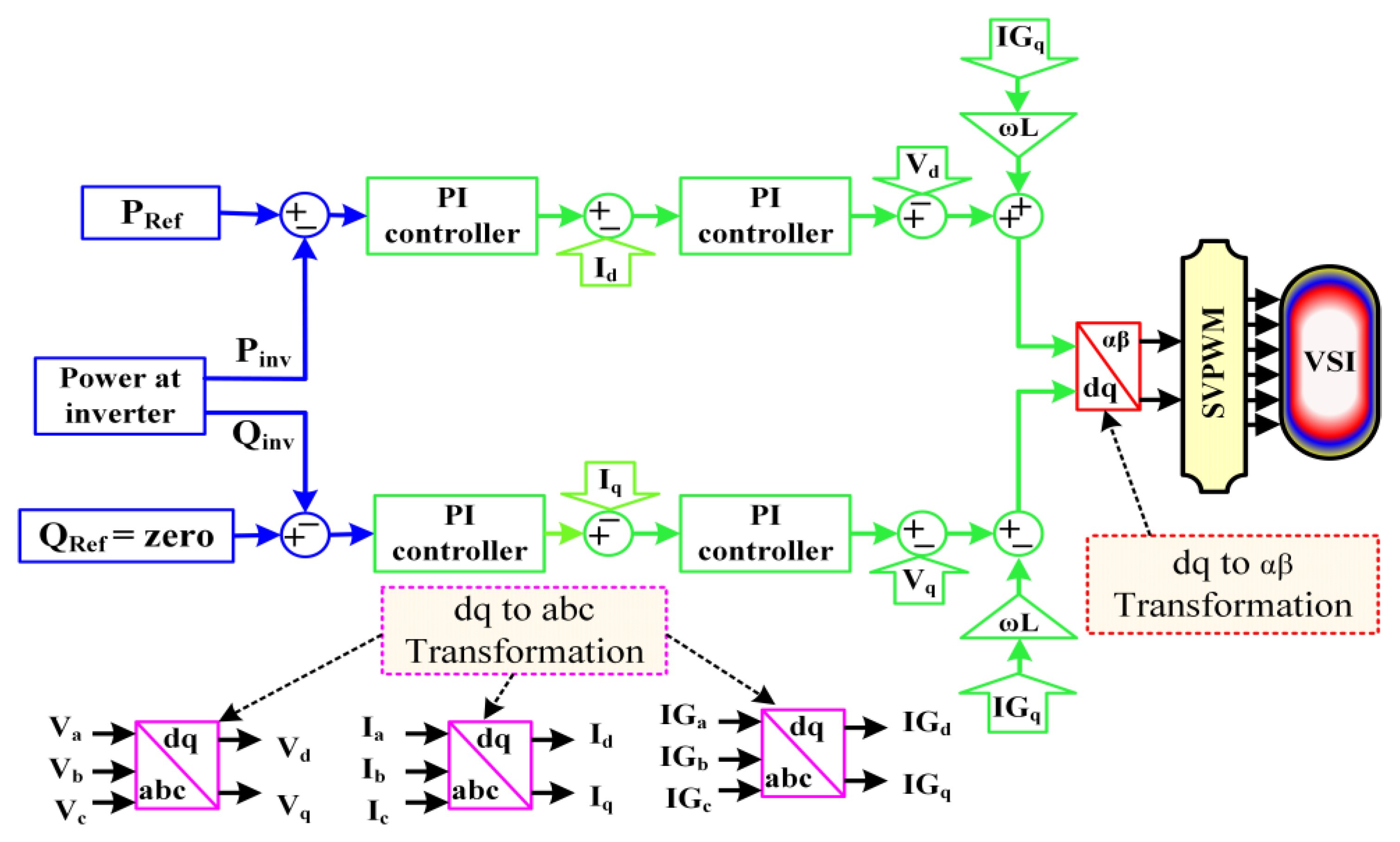
2.4. Active and Reactive Power (PQ) Control

The PQ controller utilizes PI controllers and, then converts a b c into d q reference frame which is well known as Park’s transformation [48]. This conversion is essential, since PI controllers do not perform this task with AC signals. Therefore, to obtain the desired operation of PI controllers, it must be used with DC signals or stationary transformation signals. In order to obtain the rotational angle ( ω t ), the classical phase-lock loop (PLL) has been utilized. The variable ω t is very definite for Clark’s and Park’s transformation to obtain the optimal signals of voltage and current in the d-q axis, since in the grid-connected mode of MG operation the real and reactive power is transacted between microgrid and the utility. Thus, the voltage and current of the inverter in the d-q axis are measured to check the exact power provided by the inverter [49]. The existing real and imaginary power produced by the inverter can be calculated as
P i n v = 3 2 ( v d ( i n v ) × i d ( i n v ) + v q ( i n v ) × i q ( i n v ) )
Q i n v = 3 2 ( v q ( i n v ) × i d ( i n v ) v d ( i n v ) × i q ( i n v ) )
where P i n v ,   Q i n v denote the measured active and reactive power at the inverter.
  • V d ( i n v ) , v q ( i n v ) represent the voltage of the inverter using the d-q axis.
  • i d ( i n v ) , i q ( i n v ) represent the currents in the d axis and the q axis, respectively.
In order to obtain the optimal error signals of the power, the reference real power ( P r e f ) is used in the d axis and the reference of imaginary power ( Q r e f ) is used in the q axis. After that, the error signals are evaluated using PI controllers to obtain current reference signals in the d-q axis. This procedure can be stated as
i d * = ( P r e f P i n v ) ( k p p + k i p s )
i q * = ( Q r e f Q i n v   ) ( k p q + k i q s )
where i d * , and i q * represent the current control signal after power controller in the d axis and the q axis, respectively. k p p , k i p and k p q , k i q are the gains of the power control loop PI controllers for the upper and lower arm, respectively [50].

2.5. Current Control Strategy

The main objective of utilizing the current control approach is to maintain the tracking of the reference signals of current in the d-q axis that are extracted from three phase signals of the utility [51]. This tracking depends on synchronous transformation and two PI controllers which are used to minimize the current error. Following this, the voltage of the inverter in the d-q axis is applied and then the current of the utility in the d-q axis is utilized to stabilize the steady state. The output signals from the current controller represent the optimal voltage control signal ( V d * , V q * ) synchronous frame [52]. In the synchronous d-q frame, the reference voltage signals can be expressed as
[ V d * V q * ] = [ K p ω L s ω L s K p ] [ i d i q ] + [ K p 0 0 K p ] [ i d * i q * ] + [ K i 0 0 K i ] [ X d X q ] + [ V s d V s q ]
where the superscript ‘‘*’’ denotes the reference values,
d X d d t = i d * i d ,   a n d   d X q d t = i q * i q
By applying Clarke’s transformation, we can produce clean signals in the α β frame. These signals are appropriate to be utilized with space vector pulse modulation (SVPWM) that injects the gate of VSI [53]. This can be expressed as
[ V α V β V 0 ] = 2 3 [ V a V b V c ] [ 1 1 2 0.5 0 3 2 3 2 1 2 1 2 1 2 ]
where V α , V β , and V 0 represent the voltages using the α β frame, while V a , V b , and V c represent the voltages using the a b c frame.

2.6. Space Vector Pulse Width Modulation (SVPWM)

In recent studies, the SVPWM technique is utilized with VSI network to provide the optimal pulse modulation for the VSI’s switches with a focus on the required three-phase signals [54]. The primary vector’s angle is zero, then the combination between state of the primary vector and the other vectors produces eight variant vectors that differ from the primary vector in magnitude and angle [55].

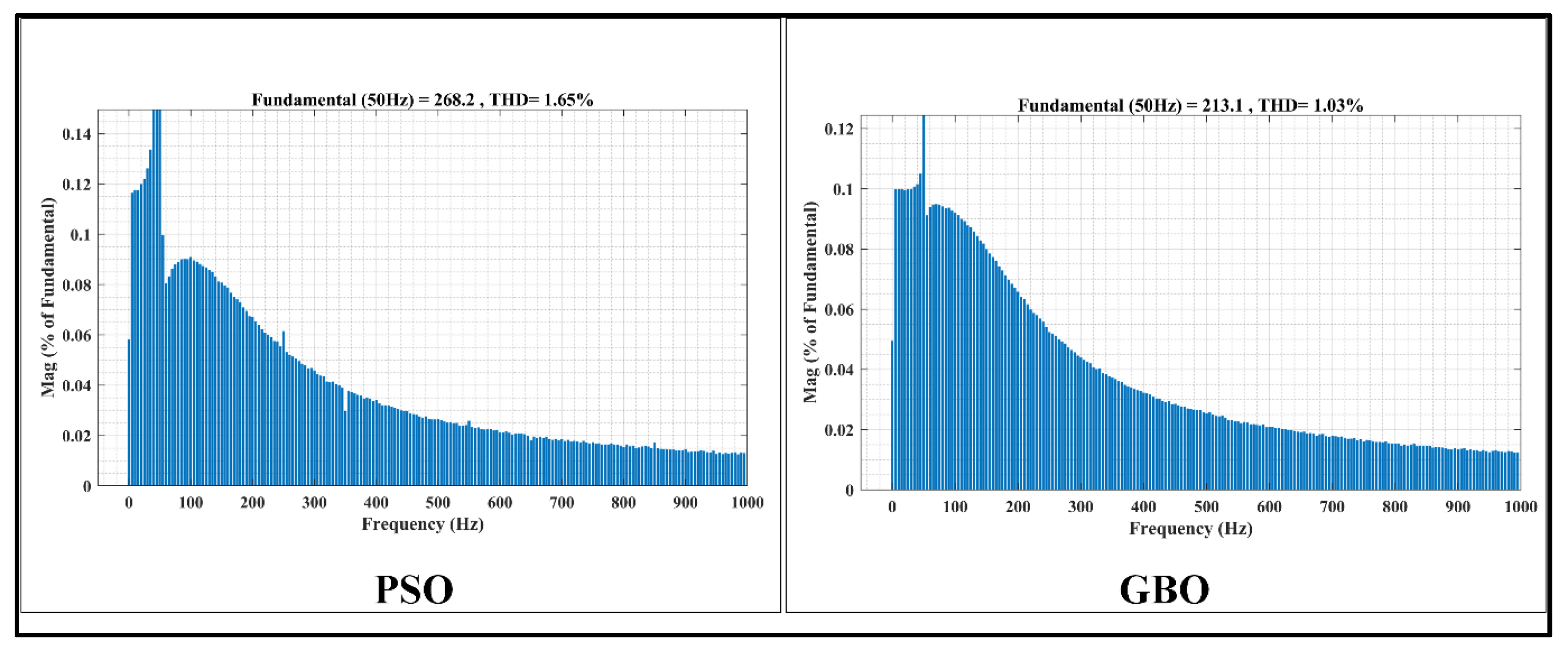
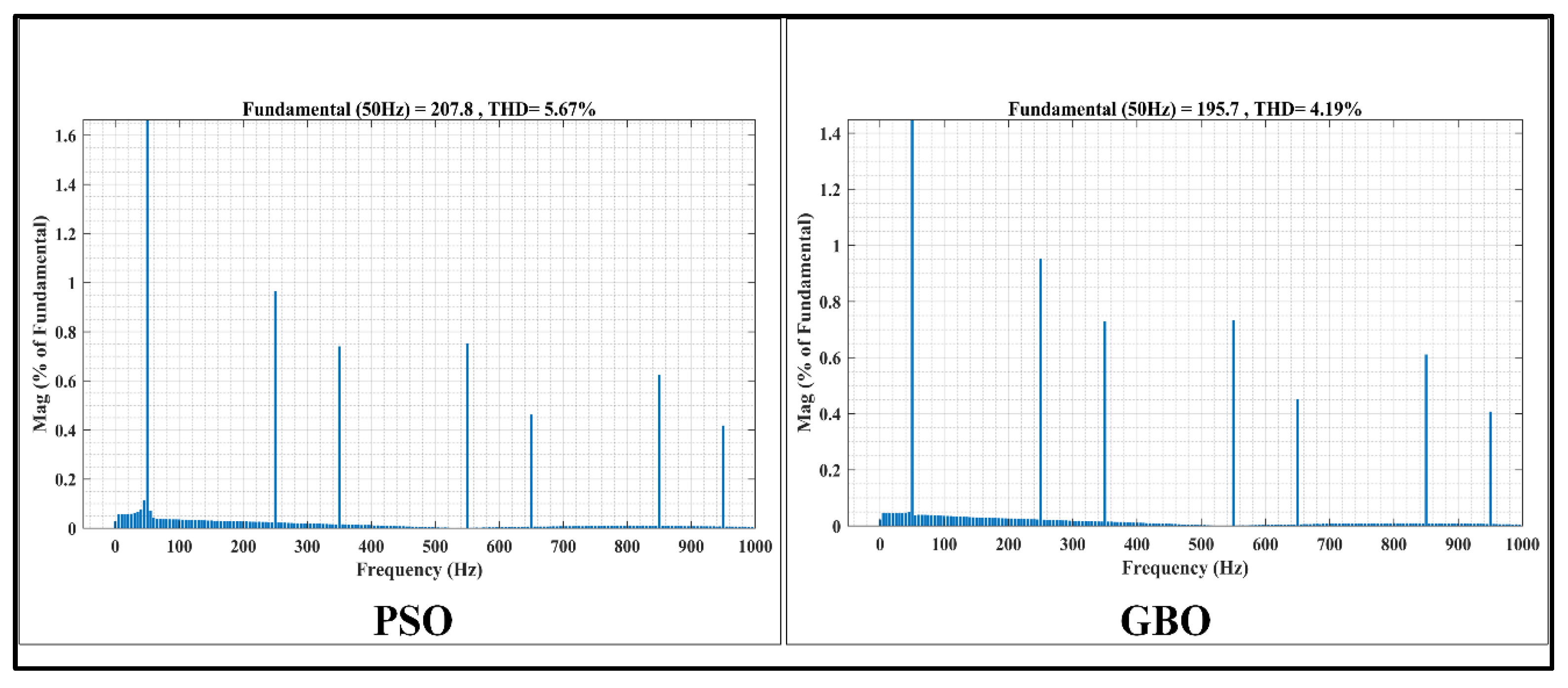
2.7. Harmonics Standard

In any network, the harmonic levels must be defined in a range to have an acceptable waveform of the measured components, such as voltage and current, whereas different kinds of loads will have different levels in %age of harmonics as it is established in different standards. These standards, such as the IEEE standard and the standards of many companies around the world, recommend the limitation of the distortion for both voltage and current [56]. In linear loads, the measured THD of the grid supply (voltage and current) is less than 5%. However, current distortion for a nonlinear load is referred to as the THD, and is taken in percentages as follows:
-
For twelve pulse devices—14% (also acceptable for modern IGBTs devices).
-
For six pulse devices—30%.
-
For four pulses devices—45% (single-phase devices) [57].

3. Optimization Procedure

The optimization process is adopted to find the optimal response of the system in different scenarios [58]. For this purpose, the particle swarm optimization algorithm (PSO) and the gradient optimization (GBO) algorithm have been used to find the optimal parameters of PI controllers in the outer loop along with two objective functions. The objective functions used ITAE and a specially developed one called ( O F ), and all of them are discussed in detail.

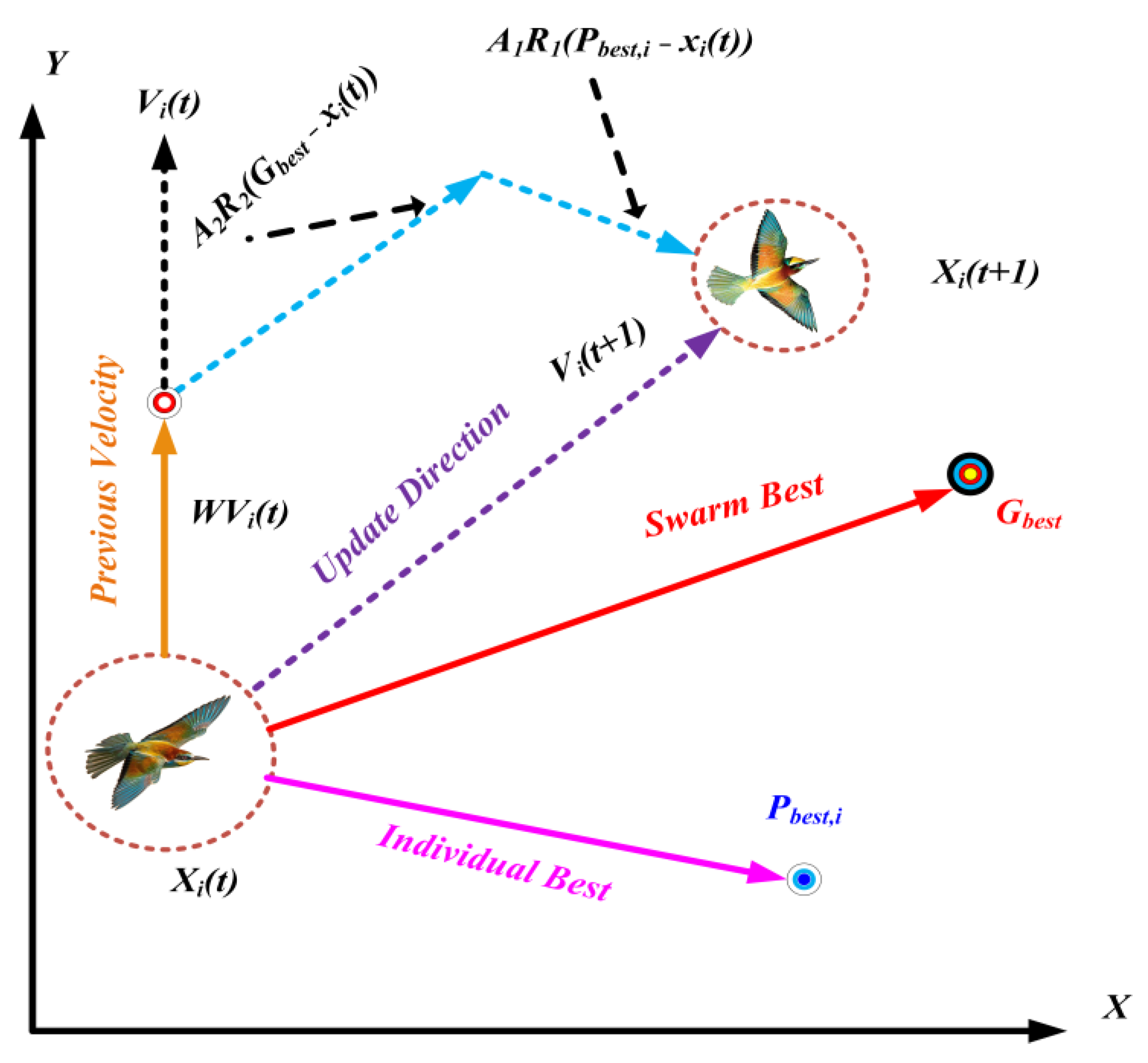
3.1. Particle Swarm Optimization (PSO) Algorithm

PSO is a benchmark metaheuristic optimization algorithm which imitates the nature of swarms of birds and was invented by Kennedy and Eberhart in 1995. It is applied to discover the search domain until it obtains the best value [59]. PSO has been utilized in several engineering fields because of its powerful search features.
The fundamental steps of the PSO algorithm can be expressed as follows:
Step 1:
Evaluating the value of the objective function for all particles.
Step 2:
Renewing local ( P b e s t , i n ) and global ( G b e s t , i n ) best values of the positions.
Step 3:
Updating the values of the velocity and positions of each particle.
Step 4:
Updating the values of the inertia and the next generation [60].
PSO procedure can be expressed depending on the following mathematical equations:
v i n ( k + 1 ) = w ( k )   v i n ( k ) + C 1 r 1 ( P b e s t , i n x i n ( k ) ) + C 2 r 2 ( G b e s t , i n x i n ( k ) )
x i n ( k + 1 ) = x i n ( k ) + v i n ( k + 1 )
where x i n ( k + 1 ) ,   x i n ( k ) are the new and former positions of the particle, respectively,   v i n ( k + 1 ) , v i n ( k ) are the new and former velocities, w ( k ) is the inertia value, P b e s t , i n is the best position for the particle ( i ) in the generation ( k ), while G b e s t , i n is the best position for the maximum number of generations. C 1 ,   C 2 are the cognitive and social learning operators. r 1 ,   r 2 are two random values in the range [0, 1]. The renewing of the direction includes three parts: previous velocity w ( k ) v i n ( k ) , particles update Λ 1 R 1 ( P b e s t , i n x i n ( k ) ) , and swarm update Λ 2 R 2 ( G b e s t , i n x i n ( k ) ) . Figure 7 illustrates the basic phenomena of particle movement toward the optimal solution [61].

3.2. Gradient Optimizer Algorithm (GBO)

GBO is one of the most modern algorithms, which contains two mechanisms: gradient search rule and local escaping operator [62]. Figure 8 portrays the sketch map of GBO.

3.2.1. Gradient Search Rule

The proposed G S R helps the GBO to account for the random behavior during the optimization process, promoting exploration and escaping local optima. The direction of movement (DM) is used to create a suitable local search tendency to promote the convergence speed of the GBO algorithm. Based on the GSR and DM, the following equation is used to update the position of the current vector ( x n m ):
X 1 n m = x n m r a n d n × ρ 1 × 2 Δ x × x n m ( x worst x b e s t + ε ) + r a n d × ρ 2 × ( x b e s t x n m )
In which   ρ 1   and   ρ 2 are given by
ρ 1 = 2 × r a n d × α α
α = | β × sin ( 3 π 2 + sin ( β × 3 π 2 ) ) |
β = β m i n + ( β m a x β m i n ) × ( 1 ( m M ) 3 ) 2
ρ 2 = 2 × r a n d × α α
where β m i n and β m a x are 0.2 and 1.2, respectively, m is the number of iterations, and M is the total number of iterations. r a n d n is a normally distributed random number, and ε is a small number within the range of [0, 0.1].
Δ x = r a n d ( 1 : N ) × | s t e p |
s t e p = ( x b e s t x r 1 m ) + δ 2
δ = 2 × r a n d × ( | x r 1 m + x r 2 m + x r 3 m + x r 4 m 4 x n m | )
where r a n d ( 1 : N ) is a random number with N dimensions, r 1 ,   r 2 ,   r 3 ,   and   r 4   ( r 1 r 2 r 3 r 4 n ) are different integers randomly chosen from [1, N], s t e p is a step size, which is determined by x b e s t and x r 1 m .
By replacing the position of the best vector ( x b e s t ) with the current vector ( x n m ) in the above equation, the new vector ( X 2 n m ) can be generated as follows:
X 2 n m = x b e s t r a n d n × ρ 1 × 2 Δ x × x n m ( y p n m y q n m + ε ) + r a n d × ρ 2 × ( x r 1 m x r 2 m )
In which
y p n = r a n d × ( [ z n + 1 + x n ] 2 + r a n d × Δ x )
y q n = r a n d × ( [ z n + 1 + x n ] 2 r a n d × Δ x )
Based on the positions X 1 n m , X 2 n m , and the current position ( X n m ) , the new solution at the next iteration ( x n m + 1 ) can be written as
x n m + 1 = r a × ( r b × X 1 n m + ( 1 r b ) × X 2 n m ) + ( 1 r a ) × X 3 n m
X 3 n m = X n m ρ 1 × ( X 2 n m X 1 n m )

3.2.2. Local Escaping Operator

Local escaping operator (LEO) is developed to increase the effectiveness of GBO. The LEO produces a solution with superior performance ( X L E O m ) by using different solutions, which contain the best position ( x b e s t ), the solutions X 1 n m and X 2 n m , two random solutions x r 1 m and x r 2 m , and a new randomly generated solution ( x k m ). The solution X L E O m is generated by the following scheme:
i f   r a n d < p r
          X L E O m = X n m + 1 + f 1 × ( u 1 × x b e s t u 2 × x k m ) + f 2 × ρ 1 × ( u 3 × ( X 2 n m X 1 n m ) + u 2 × ( x r 1 m x r 2 m ) ) / 2
X n m + 1 = X L E O m
e l s e
X L E O m = x b e s t + f 1 × ( u 1 × x b e s t u 2 × x k m ) + f 2 × ρ 1 × ( u 3 × ( X 2 n m X 1 n m ) + u 2 × ( x r 1 m x r 2 m ) ) / 2
X n m + 1 = X L E O m
e n d
e n d
where f 1 is a uniform random number in the range of [−1, 1], f 2   is a random number from a normal distribution with a mean of 0 and standard deviation of 1, p r is the probability, and u 1 , u 2 , and u 3 are three random numbers, which are defined as
u 1 = L 1 × 2 × r a n d + ( 1 L 1 )
u 2 = L 1 × r a n d + ( 1 L 1 )
u 3 = L 1 × r a n d + ( 1 L 1 )
where L 1 is a binary parameter with a value of 0 or 1. If parameter μ 1 is less than 0.5, the value of L 1 is 1, otherwise it is 0. To determine the solution x k m in Equation (35), the following scheme is suggested:
x k m = { x r a n d i f   μ 2 < 0.5 x p m o t h e r w i s e
x r a n d = X m i n + r a n d ( 0 , 1 ) × ( X m a x X m i n )
where x r a n d is a new solution, x p m is a randomly selected solution of the population ( p [ 1 ,   2 , ,   N ]), and μ 2 is a random number in the range of [0, 1]. Equations (35) and (36) can be simplified as
x k m = L 2 × x p m + ( 1 L 2 ) × x r a n d
where L 2 is a binary parameter with a value of 0 or 1. If μ 2 is less than 0.5, the value of L 2 is 1, otherwise it is 0 [63].

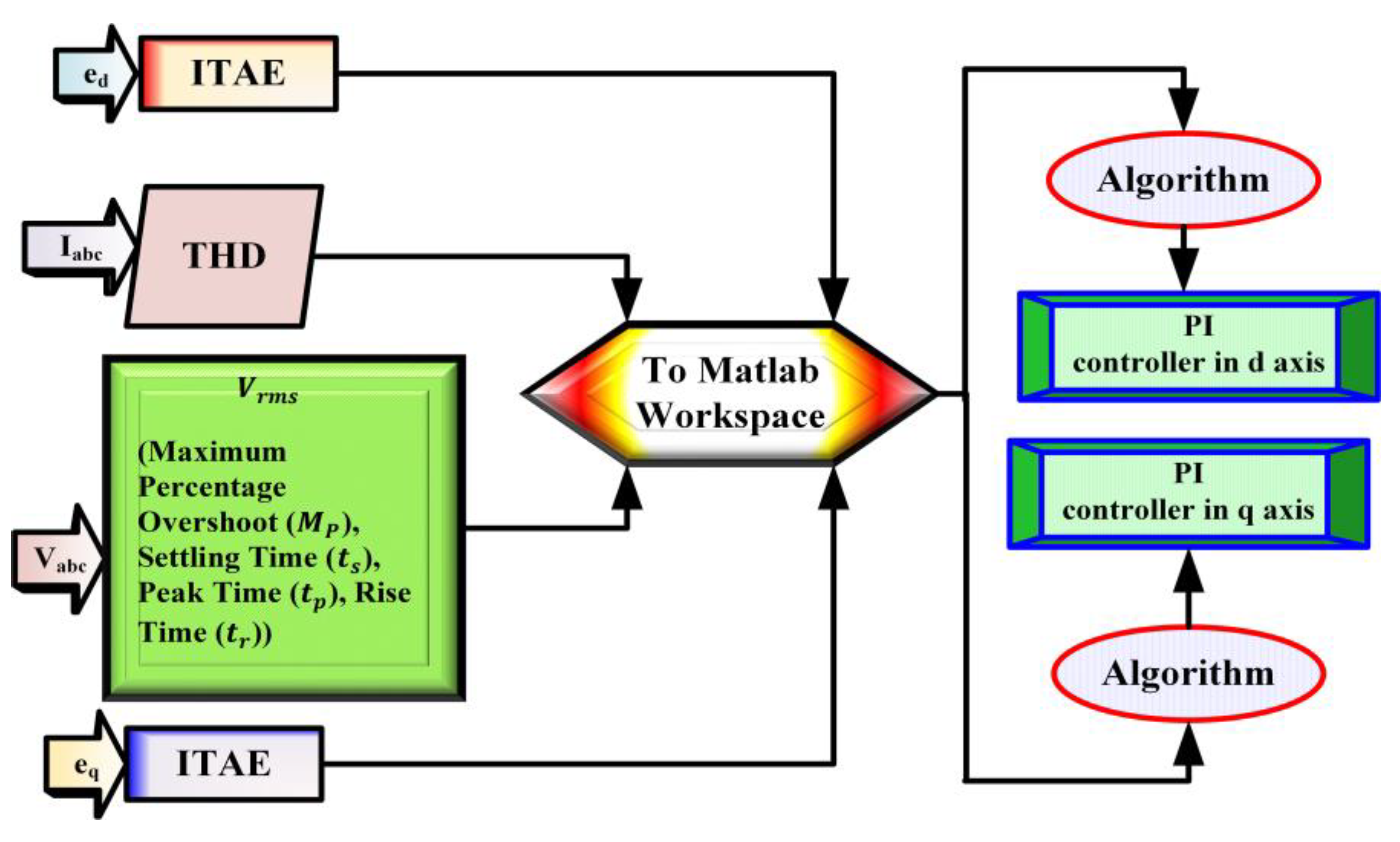
3.3. Objective Function

Integral time absolute error (ITAE) is the most used error objective function due to its advanced performance against the rivals in many cases [64]. It can be formulated in the d-axis and q-axis as:
I T A E d = 0 t | e ( t ) d |   d t
I T A E q = 0 t | e ( t ) d |   d t
I T A E T = M i n { 0 t | e ( t ) d |   d t + 0 t | e ( t ) q |   d t }
where t is the current simulation time, e ( t ) d refers to the error signal in the d axis, e ( t ) q refers to the error signal in the q axis, and I T A E T is the total ITAE function.
However, the selection of the optimal controller’s parameters depends on the design of a suitable objective function. In many studies, the fitness function is developed to accomplish the optimal execution with specific constraints: minimum overshoot/undershoot, minimum steady-state error, and THD. These novel objective functions have been examined with similar restrictions mentioned in [65,66,67].
According to that, the objective function was sensibly selected as follows:
O F = M i n { I T A E d + I T A E q + T H D I + M P + t s + t p + t r }
where I T A E d is ITAE in the d axis, I T A E q is ITAE in the q axis. From V r m s , specifications could be obtained, such as maximum overshoot ( M P ), settling time ( t s ), peak time (   t p ), and rise time ( t r ), and T H D I is the THD of the three-phase current. Figure 9 shows the objective function formulation [68]. The parameters of PI controllers required to be optimized in a grid-connected microgrid and their range are as follows:
{ 10 K P d 20 1 K I d 10 60 K P q 20 1 K I q 10
where K P d , K P q are the proportional parameters of PI controllers in the d and q axis, respectively. Similarly, K I d , K I q are the integral parameters of PI controllers in the d and q axis, respectively.

4. Results and Discussions

In this section, the case studies are introduced. Then, the tuning process using optimization algorithms to incur the advanced performance of the proposed approach is carried out. To assess the proposed control method, a microgrid system was built as shown in Figure 3 and examined using MATLAB/Simulink (R2021a) on a desktop computer running Windows 10 Enterprise 64-bit with an Intel(R) Core (TM) i5-8500 CPU processor and 8.00 GB RAM. The hyper parameters of the system are delineated in Table 2.

4.1. Case Study

The work proceeded by taking two systems during unbalanced load conditions. The system is controlled using the proposed DC voltage, active, and reactive power (DC V-P-Q) control of a grid-connected PV system through VSI.
To verify the effectiveness of the proposed method and to explain its impact in improving the power quality of the system, the proposed controller is implemented in a test applying linear load 1 at 0.05 (s), nonlinear load at the interval (0.15, 0.2) s, and unbalanced loads at 0.25 s.

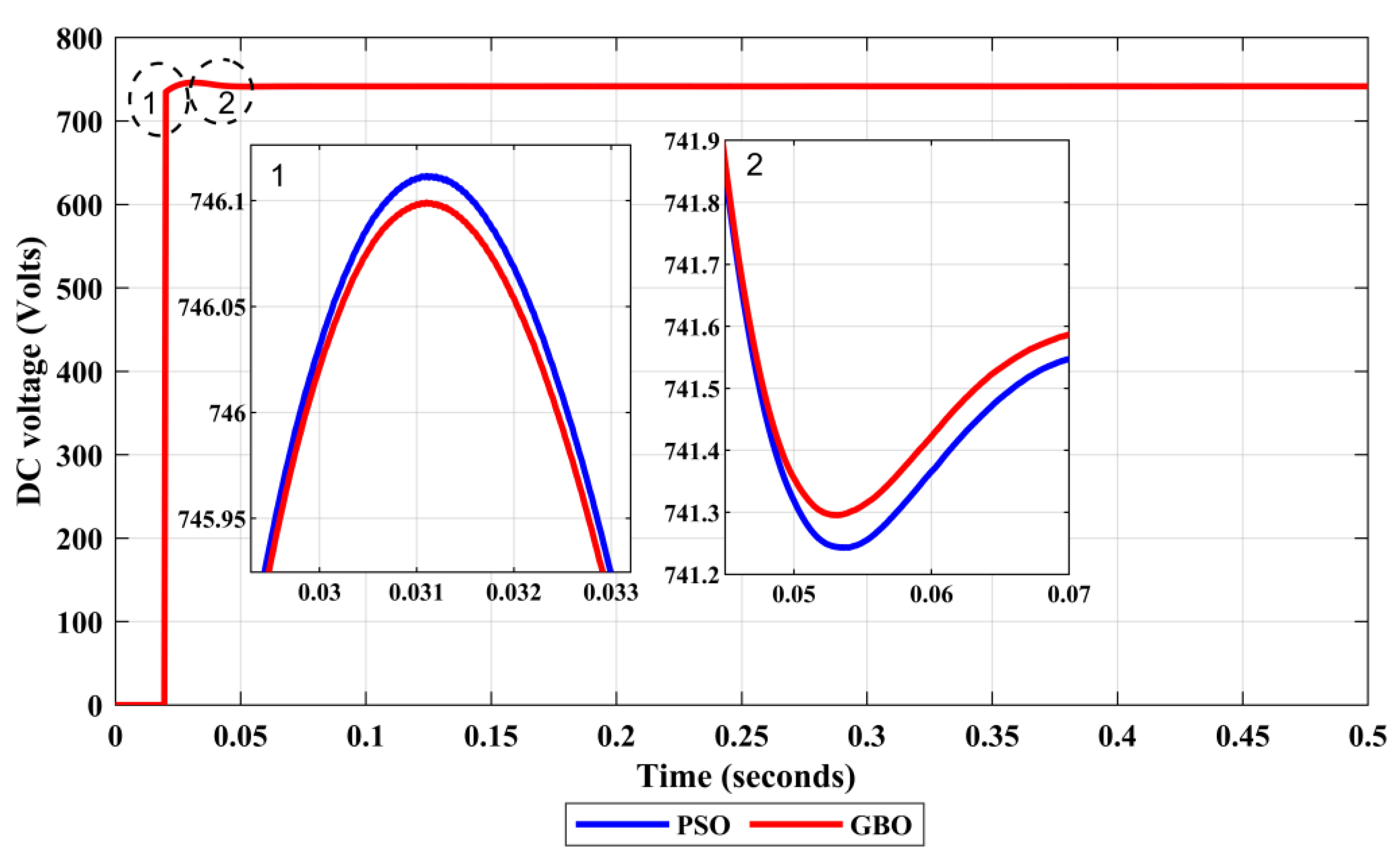
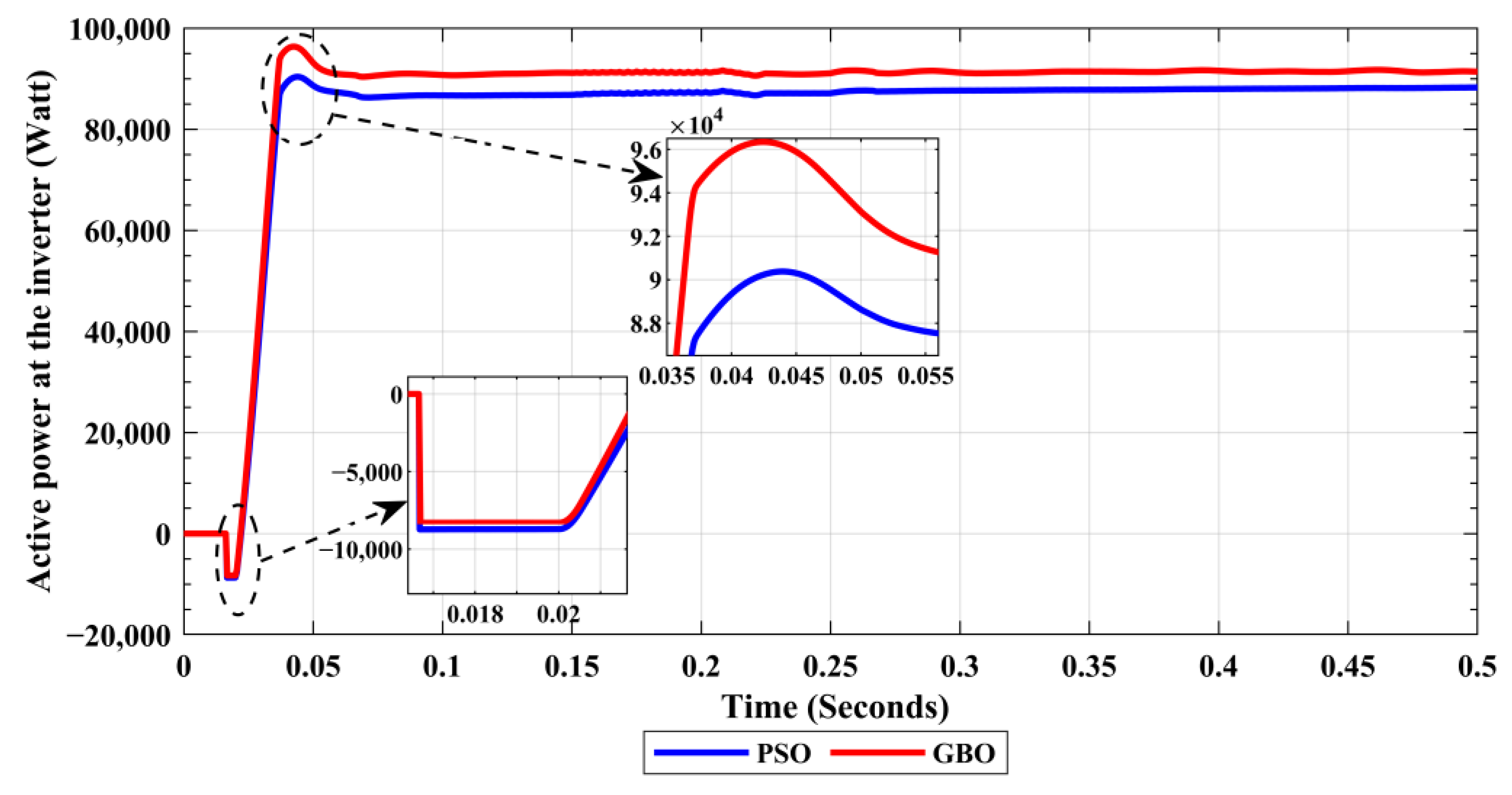
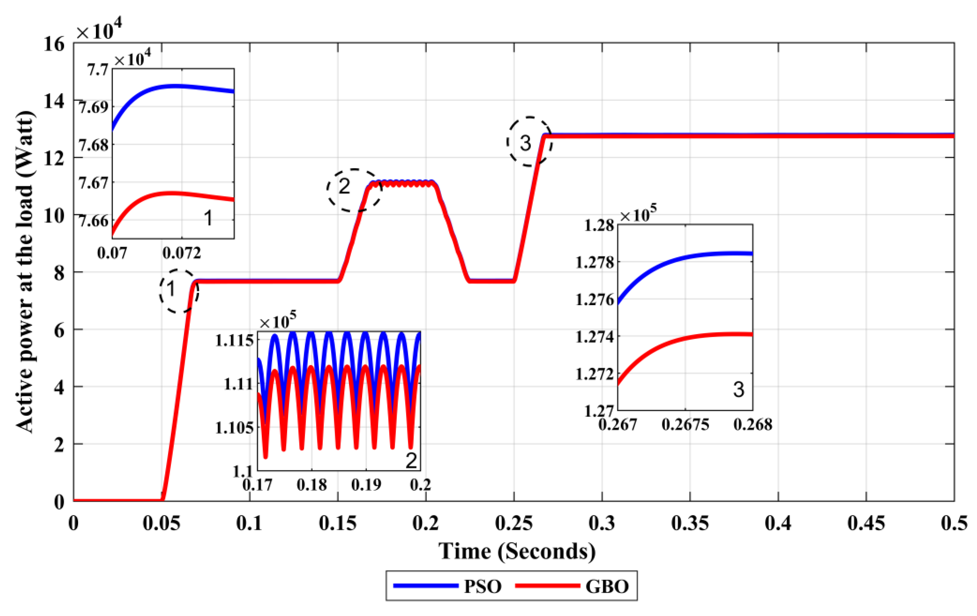
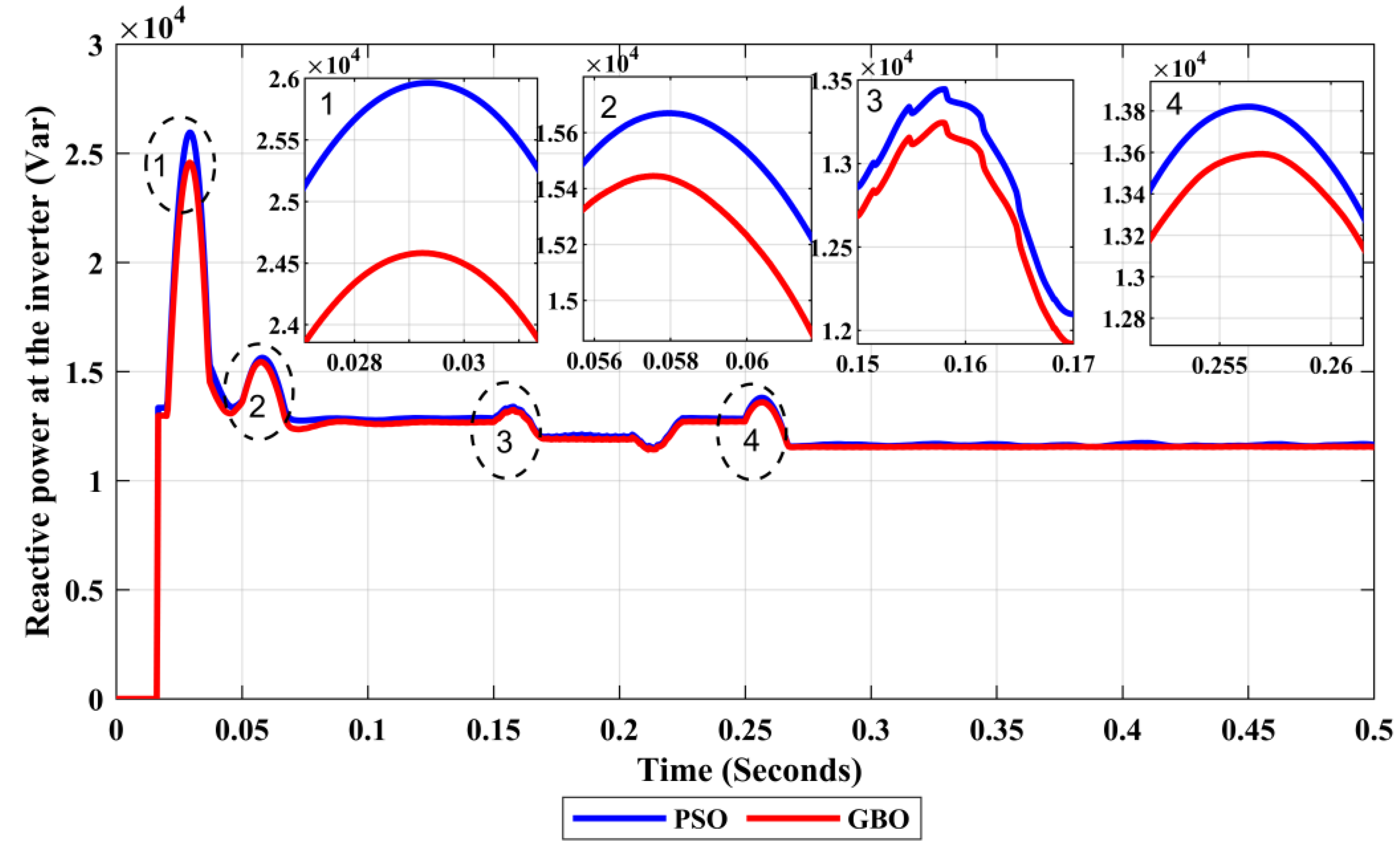
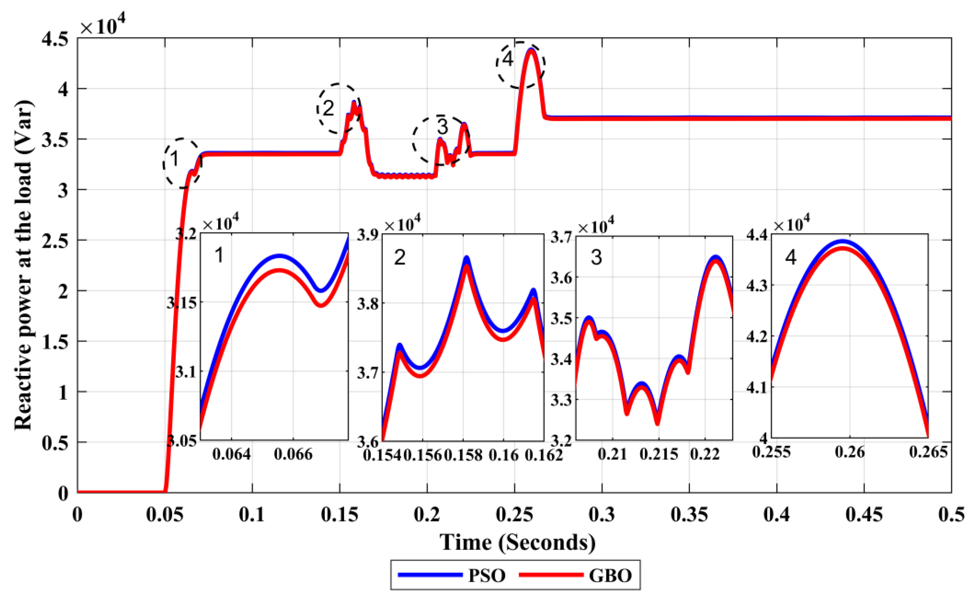
4.2. Optimization of the Grid-Interfaced Microgrid

In this sub-section, the optimization has been employed on the proposed systems in order to assess the steady-state response, dynamic response, and also the harmonic distortion.
The tuning process of PI controllers in outer loops has been achieved using PSO and GBO algorithms. The optimized parameters obtained at the end of the optimization process are provided in Table 3.
The best objective function values gained using PSO and GBO for the grid-connected microgrid are given in Figure 10. Furthermore, during the operation of the microgrid with load demand change, the given algorithms provide stability to the system. It can be observed that GBO demonstrates early and high-speed convergence compared to the competitors because of its covenant arrangement for the exploration and exploitation process.
Figure 11 demonstrates tuned DC voltage in a grid-connected microgrid. The proposed control method maintains the DC voltage rate within the acceptable range around the nominal DC voltage. However, GBO obtains the best signal response in terms of fast response, and less value in both overshoot and undershoot value.
To verify the optimal control of the real power, Figure 12 illustrates the real power signal at the inverter in different scenarios. The DG unit keeps its output stable, which proves the validity of the proposed control method. The microgrid meets the total load demand based on its maximum generated power by PV. Henceforth, GBO obtained the best active power wave injected from the PV system.
Figure 13 demonstrates the active power signal at load in the tuned grid-connected microgrid, whereas the proposed method-based algorithms have pumps of equivalent value of active power to the load. Moreover, the rate of active power is updated with the same rate when the load has changed after competing for the desired power from the utility, whereas the proposed controller-based GBO confirms the robust tracking behavior during the variation of the load.
The proposed controller inserts the reactive power depending on the reference value, which is zero, to keep the reactive value near zero. Moreover, self-tuning by different algorithms provides equal load sharing between the microgrid and upstream during load changes (linear load 1, nonlinear load, and linear load 2). Moreover, the GBO-based controller achieves the target with the best dynamic response among its counterparts. Figure 14 depicts the tuned reactive power signal at the inverter in the grid-connected microgrid.
Figure 15 shows the reactive power signal at load in the tuned grid-connected microgrid. Reactive power-sharing between the grid-supporting VSIs is confirmed during different scenarios, whilst the proposed method-based PSO is significantly high compared to the case of the proposed method-based GBO.
The enhancement of the transient response in the disturbance interval points to the possession of a sufficient power quality for the system requirements for the connection between the PV system and the utility grid as recommended by the standards. Table 4 shows a comparison between controller-based PSO and GBO in terms of transient response.
In order to justify the optimal dynamic response, the current of the system is examined three times within ten cycles. The first time was during inserting the linear load 1 at 0.05 s. Second was during inserting the nonlinear load in the interval between 0.15 and 0.2 s. The third was at 0.25 s, along with inserting linear load 2. The results show that pure sinusoidal waves with high quality in different algorithms were used along with the proposed method, whereas the GBO-based control method obtained the best results. Figure 16 shows the THD of line current of the tuned grid-interfaced PV after inserting linear load 1, Figure 17 illustrates the THD of line current of the tuned grid-interfaced PV after inserting nonlinear load, and Figure 18 displays the THD of line current of the tuned grid-interfaced PV after inserting linear load 2.
This study delivers a brief analysis of the proposed method, and tuning using optimization algorithms. The design of the objective function plays a significant role in the optimization process to obtain the optimal transient response and adjust power sharing between PV units and the utility grid. In addition, the proposed method-based GBO has achieved the best shaving of the peak of the load power by lessening the desired power from the utility grid, eliminating short duration power spikes.

5. Conclusions and Future Work

This work adopted a comprehensive analysis based on a combination of DC voltage, active power, and reactive power control (DC V-P-Q), in order to achieve an optimal regulation of DC voltage and active and reactive power. Hence, the DC microgrid maintains a constant voltage at the DC link capacitor and mitigates the power quality issues of the microgrid. Moreover, the performance of the transfer of energy based on the real and reactive power between the microgrid and the utility varied across during different scenarios. The results prove the perfection of controlling DC voltage and real and reactive power.
The application of metaheuristics enhanced the overall decision order ability and minimized the complication burden. Moreover, the results show that the proposed method-based GBO has improved with the fastest optimal transient response in different operation requirements in the grid-connected photovoltaic system. The THD percentage for the PSO technique was 1.65%, 5.67%, and 1.13% during load disturbances [load 1, load 2, and load 3], while the THD percentage for the GBO approach was 1.03%, 4.19%, and 0.42% during the same load disturbances, respectively.
In future work, it would be valuable to further enhance and investigate the following aspects: (i) Whether the GBO algorithm can be modified and other intelligent algorithms can be used and developed to attain faster convergence and lower harmonics. (ii) Hardware tests can be conducted to validate the efficiency of the proposed approaches.

Author Contributions

Conceptualization, S.M.A.A.; Methodology, S.M.A.A.; Software, S.M.A.A.; Validation, S.M.A.A.; Writing—original draft, S.M.A.A.; Writing—review & editing, N.H., A.Y., S.A.H., R.H.A. and L.M.; Supervision, A.S.B.M. and S.B.A.K. All authors have read and agreed to the published version of the manuscript.

Funding

This research received no external funding.

Data Availability Statement

Not applicable.

Acknowledgments

The first author thanks the Libyan government for supporting this research with a scholarship provided by the Ministry of Higher Education and Scientific Research. The authors would like to acknowledge the facilities provided by Universiti Teknologi Malaysia for the accomplishment of this work. The authors would like to thank the editor and anonymous reviewers for improving this paper with their valuable comments and suggestions.

Conflicts of Interest

The authors declare no conflict of interest.

Nomenclature

Symbols
V D C DC voltage
T s sample time
f S Switch frequency
K P d Proportional parameter of PI controller in d vector
K P q Proportional parameter of PI controller in q vector
K I d Integral parameter of PI controller in d vector
K I q Integral parameter of PI controller in q vector
e ( t ) d Error in in d vector
e ( t ) q Error in in q vector
Abbreviations
PVPhotovoltaic
VSIVoltage source inverter
PIproportional integral
PIDProportional integral derivative
PSOParticle swarm optimization
IGBTInsulated gate bipolar transistor
ITAEIntegral time absolute error
rmsRoot mean square
P&OPerturb and observe
MPPTMaximum power point tracking
SVPWMSpace vector pulse width modulation
OF Objective function
GBOGradient-base optimizer
DC V-P-QDC Voltage, active and reactive power

References

  1. Luo, F.L.; Hong, Y. Advanced DC/AC Inverters: Applications in Renewable Energy; CRC Press: Boca Raton, FL, USA, 2017; pp. 1–319. [Google Scholar]
  2. Memon, A.; Wazir Bin Mustafa, M.; Anjum, W.; Ahmed, A.; Ullah, S.; Altbawi, S.M.A.; Jumani, T.A.; Khan, I.; Hamadneh, N.N. Dynamic response and low voltage ride-through enhancement of brushless double-fed induction generator using Salp swarm optimization algorithm. PLoS ONE 2022, 17, e0265611. [Google Scholar] [CrossRef]
  3. Zeb, K.; Uddin, W.; Khan, M.A.; Ali, Z.; Ali, M.U.; Christofides, N.; Kim, H.J. A comprehensive review on inverter topologies and control strategies for grid connected photovoltaic system. Renew. Sustain. Energy Rev. 2018, 94, 1120–1141. [Google Scholar] [CrossRef]
  4. Ahmed, M.; Harbi, I.; Kennel, R.; Rodríguez, J.; Abdelrahem, M. Evaluation of the Main Control Strategies for Grid-Connected PV Systems. Sustainability 2022, 14, 1142. [Google Scholar] [CrossRef]
  5. Wang, Y.; Nguyen, T.L.; Xu, Y.; Li, Z.; Tran, Q.T.; Caire, R. Cyber-Physical Design and Implementation of Distributed Event-Triggered Secondary Control in Islanded Microgrids. IEEE Trans. Ind. Appl. 2019, 55, 5631–5642. [Google Scholar] [CrossRef]
  6. Li, Z.; Xu, Y.; Feng, X.; Wu, Q. Optimal Stochastic Deployment of Heterogeneous Energy Storage in a Residential Multienergy Microgrid with Demand-Side Management. IEEE Trans. Ind. Inform. 2021, 17, 991–1004. [Google Scholar] [CrossRef]
  7. Cheng, X.; Zheng, Y.; Lin, Y.; Chen, L.; Wang, Y.; Qiu, J. Hierarchical operation planning based on carbon-constrained locational marginal price for integrated energy system. Int. J. Electr. Power Energy Syst. 2021, 128, 106714. [Google Scholar] [CrossRef]
  8. Wang, Z.; Fu, P.; Huang, L.; Chen, X.; He, S.; Wang, Z.; Chen, T.; Wang, Z.; Tong, W. Unified power control strategy for new generation poloidal field power supply. Fusion Eng. Des. 2021, 168, 112404. [Google Scholar] [CrossRef]
  9. Dozein, M.G.; Gomis-Bellmunt, O.; Mancarella, P. Simultaneous Provision of Dynamic Active and Reactive Power Response from Utility-Scale Battery Energy Storage Systems in Weak Grids. IEEE Trans. Power Syst. 2021, 36, 5548–5557. [Google Scholar] [CrossRef]
  10. Šimek, P.; Bejvl, M.; Valouch, V. Power control for grid-connected converter based on generalized predictive current control. IEEE J. Emerg. Sel. Top. Power Electron. 2022, 10, 7072–7083. [Google Scholar] [CrossRef]
  11. Imam, A.A.; Sreerama Kumar, R.; Al-Turki, Y.A. Modeling and simulation of a pi controlled shunt active power filter for power quality enhancement based on p-q theory. Electronics 2020, 9, 637. [Google Scholar] [CrossRef]
  12. Ma, D.; Cao, X.; Sun, C.; Wang, R.; Sun, Q.; Xie, X.; Peng, W. Dual-Predictive Control With Adaptive Error Correction Strategy for AC Microgrids. IEEE Trans. Power Deliv. 2022, 37, 1930–1940. [Google Scholar] [CrossRef]
  13. Monshizadeh, N.; Mancilla-David, F.; Ortega, R.; Cisneros, R. Nonlinear Stability Analysis of the Classical Nested PI Control of Voltage Sourced Inverters. IEEE Control Syst. Lett. 2022, 6, 1442–1447. [Google Scholar] [CrossRef]
  14. Khomsi, C.; Bouzid, M.; Jelassi, K. Power quality improvement in a three-phase grid tied photovoltaic system supplying unbalanced and nonlinear loads. Int. J. Renew. Energy Res. 2018, 8, 1165–1177. [Google Scholar] [CrossRef]
  15. Ansari, M.N.; Singh, R.K. Application of D-STATCOM for Harmonic Reduction using Power Balance Theory. Turk. J. Comput. Math. Educ. TURCOMAT 2021, 12, 2496–2503. [Google Scholar] [CrossRef]
  16. Sun, L.; Jin, Y.; Pan, L.; Shen, J.; Lee, K.Y. Efficiency analysis and control of a grid-connected PEM fuel cell in distributed generation. Energy Convers. Manag. 2019, 195, 587–596. [Google Scholar] [CrossRef]
  17. Duarte, S.N.; Almeida, P.M.; Barbosa, P.G. Voltage regulation of a remote microgrid bus with a modular multilevel STATCOM. Electr. Power Syst. Res. 2022, 212, 108299. [Google Scholar] [CrossRef]
  18. Singh, B.; Shah, P.; Hussain, I. ISOGI-Q Based Control Algorithm for a Single Stage Grid Tied SPV System. IEEE Trans. Ind. Appl. 2018, 54, 1136–1145. [Google Scholar] [CrossRef]
  19. Shah, P.; Hussain, I.; Singh, B. Single-Stage SECS interfaced with grid using ISOGI-FLL-based control algorithm. IEEE Trans. Ind. Appl. 2019, 55, 701–711. [Google Scholar] [CrossRef]
  20. Agarwal, R.K.; Hussain, I.; Singh, B. LMF-based control algorithm for single stage three-phase grid integrated solar PV system. IEEE Trans. Sustain. Energy 2016, 7, 1379–1387. [Google Scholar] [CrossRef]
  21. Agarwal, R.K.; Hussain, I.; Singh, B. Implementation of LLMF Control Algorithm for Three-Phase Grid-Tied SPV-DSTATCOM System. IEEE Trans. Ind. Electron. 2017, 64, 7414–7424. [Google Scholar] [CrossRef]
  22. Kumar, N.; Singh, B.; Panigrahi, B.K. LLMLF-Based Control Approach and LPO MPPT Technique for Improving Performance of a Multifunctional Three-Phase Two-Stage Grid Integrated PV System. IEEE Trans. Sustain. Energy 2020, 11, 371–380. [Google Scholar] [CrossRef]
  23. Badoni, M.; Singh, A.; Singh, B. Comparative Performance of Wiener Filter and Adaptive Least Mean Square-Based Control for Power Quality Improvement. IEEE Trans. Ind. Electron. 2016, 63, 3028–3037. [Google Scholar] [CrossRef]
  24. Wang, G.; Wang, X.; Lv, J. An Improved Harmonic Suppression Control Strategy for the Hybrid Microgrid Bidirectional AC/DC Converter. IEEE Access 2020, 8, 220422–220436. [Google Scholar] [CrossRef]
  25. Ray, P.K. Power Quality Improvement Using VLLMS Based Adaptive Shunt Active Filter. CPSS Trans. Power Electron. Appl. 2018, 3, 154–162. [Google Scholar] [CrossRef]
  26. Hussain, I.; Agarwal, R.K.; Singh, B. MLP Control Algorithm for Adaptable Dual-Mode Single-Stage Solar PV System Tied to Three-Phase Voltage-Weak Distribution Grid. IEEE Trans. Ind. Inf. 2018, 14, 2530–2538. [Google Scholar] [CrossRef]
  27. Chawda, G.S.; Shaik, A.G.; Mahela, O.P.; Padmanaban, S.; Holm-Nielsen, J.B. Comprehensive Review of Distributed FACTS Control Algorithms for Power Quality Enhancement in Utility Grid With Renewable Energy Penetration. IEEE Access 2020, 8, 107614–107634. [Google Scholar] [CrossRef]
  28. Khorramabadi, S.S.; Bakhshai, A. Critic-Based Self-Tuning PI Structure for Active and Reactive Power Control of VSCs in Microgrid Systems. IEEE Trans. Smart Grid 2014, 6, 92–103. [Google Scholar] [CrossRef]
  29. Balasubramanian, R.; Sankaran, R.; Palani, S. Simulation and performance evaluation of shunt hybrid power filter using fuzzy logic based non-linear control for power quality improvement. Sadhana Acad. Proc. Eng. Sci. 2017, 42, 1443–1452. [Google Scholar] [CrossRef]
  30. Tali, M.; Esadki, A.; Nasser, T.; Boukezata, B. Active power filter for power quality in grid connected PV-system using an improved fuzzy logic control MPPT. In Proceedings of the 2018 6th International Renewable and Sustainable Energy Conference, IRSEC 2018, Rabat, Morocco, 5–8 December 2018. [Google Scholar] [CrossRef]
  31. Shan, Y.; Hu, J.; Liu, H. A Holistic Power Management Strategy of Microgrids Based on Model Predictive Control and Particle Swarm Optimization. IEEE Trans. Ind. Inform. 2021, 18, 5115–5126. [Google Scholar] [CrossRef]
  32. Durairasan, M.; Balasubramanian, D. An efficient control strategy for optimal power flow management from a renewable energy source to a generalized three-phase microgrid system: A hybrid squirrel search algorithm with whale optimization algorithm approach. Trans. Inst. Meas. Control 2020, 42, 1960–1976. [Google Scholar] [CrossRef]
  33. Ramadan, H.S.; Padmanaban, S.; Mosaad, M.I. Metaheuristic-based Near-Optimal Fractional Order PI Controller for On-grid Fuel Cell Dynamic Performance Enhancement. Electr. Power Syst. Res. 2022, 208, 107897. [Google Scholar] [CrossRef]
  34. Sameh, M.A.; Marei, M.I.; Badr, M.A.; Attia, M.A. An Optimized PV Control System Based on the Emperor Penguin Optimizer. Energies 2021, 14, 751. [Google Scholar] [CrossRef]
  35. Abdolrasol, M.G.; Ayob, A.; Mutlag, A.H.; Ustun, T.S. Optimal fuzzy logic controller based PSO for photovoltaic system. Energy Rep. 2023, 9, 427–434. [Google Scholar] [CrossRef]
  36. Arfeen, Z.A.; Kermadi, M.; Azam, M.K.; Siddiqui, T.A.; Akhtar, Z.U.; Ado, M.; Abdullah, P. Insights and trends of optimal voltage-frequency control DG-based inverter for autonomous microgrid: State-of-the-art review. Int. Trans. Electr. Energy Syst. 2020, 30, 1–26. [Google Scholar] [CrossRef]
  37. Altbawi, S.M.A.; Mokhtar, A.S.; Arfeen, Z.A. Enhacement of microgrid technologies using various algorithms. Turk. J. Comput. Math. Educ. 2021, 12, 1127–1170. [Google Scholar]
  38. Hamrouni, N.; Jraidi, M.; Chérif, A. New method of current control for LCL-interfaced grid-connected three phase voltage source inverter. Rev. Énergie. Renouvelables 2010, 13, 1–14. [Google Scholar]
  39. Geury, T.; Pinto, S.; Gyselinck, J. Three-phase power controlled PV current source inverter with incorporated active power filtering. In Proceedings of the IECON 2013—39th Annual Conference of the IEEE Industrial Electronics Society, Vienna, Austria, 10–13 November 2013; pp. 1374–1379. [Google Scholar] [CrossRef]
  40. Jumani, T.A.; Mustafa, M.W.; Rasid, M.; Mirjat, N.H.; Baloch, M.H.; Salisu, S. Optimal Power Flow Controller for Grid-Connected Microgrids using Grasshopper Optimization Algorithm. Electronics 2019, 8, 111. [Google Scholar] [CrossRef]
  41. Zeng, Z.; Yang, H.; Zhao, R.; Cheng, C. Topologies and control strategies of multi-functional grid-connected inverters for power quality enhancement: A comprehensive review. Renew. Sustain. Energy Rev. 2013, 24, 223–270. [Google Scholar] [CrossRef]
  42. Harrag, A.; Messalti, S. PSO-based SMC variable step size P&O MPPT controller for PV systems under fast changing atmospheric conditions. Int. J. Numer. Model. Electron. Netw. Devices Fields 2019, 32, e2603. [Google Scholar] [CrossRef]
  43. Bhattacharyya, S.; Kumar, P.D.S.; Samanta, S.; Mishra, S. Steady Output and Fast Tracking MPPT (SOFT-MPPT) for P&O and InC Algorithms. IEEE Trans. Sustain. Energy 2021, 12, 293–302. [Google Scholar] [CrossRef]
  44. Zhu, Y.L.; Yao, J.G.; Wu, D. Comparative study of two stages and single stage topologies for grid-tie photovoltaic generation by PSCAD/EMTDC. In Proceedings of the 2011 International Conference on Advanced Power System Automation and Protection, Beijing, China, 16–20 October 2011; Volume 2, pp. 1304–1309. [Google Scholar] [CrossRef]
  45. Aijaz, M.; Hussain, I.; Lone, S.A. Golden Eagle Optimized Control for a Dual Stage Photovoltaic Residential System with Electric Vehicle Charging Capability. Energy Sources Part A Recover. Util. Environ. Eff. 2022, 44, 4525–4545. [Google Scholar] [CrossRef]
  46. Keshta, H.E.; Saied, E.M.; Malik, O.P.; Bendary, F.M.; Ali, A.A. Fuzzy PI controller-based model reference adaptive control for voltage control of two connected microgrids. IET Gener. Transm. Distrib. 2020, 15, 602–618. [Google Scholar] [CrossRef]
  47. Mehta, G.; Singh, S. Design of single-stage three-phase grid-connected photovoltaic system with MPPT and reactive power compensation control. Int. J. Power Energy Convers. 2014, 5, 211–227. [Google Scholar] [CrossRef]
  48. Mahdavi, M.S.; Gharehpetian, G.B.; Ghasemi, A. An Enhanced Converter-based Diesel Generator Emulator for Voltage and Frequency Control Studies in Laboratory-Scale Microgrids. Iran. J. Sci. Technol. Trans. Electr. Eng. 2021, 45, 945–957. [Google Scholar] [CrossRef]
  49. Sureshkumar, K.; Ponnusamy, V. Power flow management in micro grid through renewable energy sources using a hybrid modified dragonfly algorithm with bat search algorithm. Energy 2019, 181, 1166–1178. [Google Scholar] [CrossRef]
  50. Mahmoud, M.S.; Hussain, S.A. Adaptive PI secondary control for smart autonomous microgrid systems. Int. J. Adapt. Control Signal Process. 2015, 29, 1442–1458. [Google Scholar] [CrossRef]
  51. Yang, Y.; Yang, P. A novel strategy for improving power quality of islanded hybrid AC/DC microgrid using parallel-operated interlinking converters. Int. J. Electr. Power Energy Syst. 2022, 138, 107961. [Google Scholar] [CrossRef]
  52. Bo, L.; Huang, L.; Dai, Y.; Lu, Y.; Chong, K.T. Mitigation of DC Components Using Adaptive BP-PID Control in Transformless Three-Phase Grid-Connected Inverters. Energies 2018, 11, 2047. [Google Scholar] [CrossRef]
  53. Kakkar, S.; Ahuja, R.K.; Maity, T. Performance enhancement of grid-interfaced inverter using intelligent controller. Meas. Control 2020, 53, 551–563. [Google Scholar] [CrossRef] [Green Version]
  54. Wu, X.; Xiong, C.; Yang, S.; Yang, H.; Feng, X. A Simplified Space Vector Pulsewidth Modulation Scheme for Three-Phase Cascaded H-Bridge Inverters. IEEE Trans. Power Electron. 2019, 35, 4192–4204. [Google Scholar] [CrossRef]
  55. Lewicki, A.; Odeh, C.; Morawiec, M. Space Vector Pulsewidth Modulation Strategy for Multilevel Cascaded H-Bridge Inverter With DC-Link Voltage Balancing Ability. IEEE Trans. Ind. Electron. 2022, 70, 1161–1170. [Google Scholar] [CrossRef]
  56. IEEE. IEEE Standard 519-2014, IEEE, 1–50, 2014, [Online]. Available online: https://www.schneider-electric.com.tw/documents/Event/2016_electrical_engineering_seminar/IEEE_STD_519_1992vs2014.pdf (accessed on 16 January 2022).
  57. Technologies, C.G. AGN 025—Non Linear Loads, Cummins Generator Technologies. Available online: https://www.stamford-avk.com/sites/stamfordavk/files/AGN025_B.pdf (accessed on 28 January 2022).
  58. Mirjalili, S. Evolutionary Algorithms and Neural Networks, 1st ed.; Springer International Publishing: New York, NY, USA, 2019. [Google Scholar] [CrossRef]
  59. Kennedy, J.; Eberhart, R. Particle swarm optimization. In Proceedings of the ICNN’95-International Conference on Neural Networks, Perth, WA, Australia, 27 November–1 December 1995; Volume 4, pp. 1942–1948. [Google Scholar]
  60. Shi, Y.; Eberhart, R. A modified particle swarm optimizer. In Proceedings of the 1998 IEEE International Conference on Evolutionary Computation Proceedings. IEEE World Congress on Computational Intelligence (Cat. No. 98TH8360), Anchorage, AK, USA, 4–9 May 1998; pp. 69–73. [Google Scholar]
  61. Bakht, M.P.; Salam, Z.; Bhatti, A.R.; Ullah Sheikh, U.; Khan, N.; Anjum, W. Techno-economic modelling of hybrid energy system to overcome the load shedding problem: A case study of Pakistan. PLoS ONE 2022, 17, e0266660. [Google Scholar] [CrossRef] [PubMed]
  62. Ahmadianfar, I.; Bozorg-Haddad, O.; Chu, X. Gradient-based optimizer: A new metaheuristic optimization algorithm. Inf. Sci. 2020, 540, 131–159. [Google Scholar] [CrossRef]
  63. Premkumar, M.; Jangir, P.; Sowmya, R. MOGBO: A new Multiobjective Gradient-Based Optimizer for real-world structural optimization problems. Knowl. Based Syst. 2021, 218, 106856. [Google Scholar] [CrossRef]
  64. Mohamed, R.G.; Ebrahim, M.A.; Alaas, Z.M.; Ahmed, M.M.R. Optimal Energy Harvesting of Large-Scale Wind Farm Using Marine Predators Algorithm. IEEE Access 2022, 10, 24995–25004. [Google Scholar] [CrossRef]
  65. Ebrahim, M.A.; Ayoub, B.A.A.; Nashed, M.N.F.; Osman, F.A.M. A Novel Hybrid-HHOPSO Algorithm Based Optimal Compensators of Four-Layer Cascaded Control for a New Structurally Modified AC Microgrid. IEEE Access 2020, 9, 4008–4037. [Google Scholar] [CrossRef]
  66. Ebrahim, M.A.; Aziz, B.A.; Nashed, M.N.; Osman, F. Optimal design of controllers and harmonic compensators for three-level cascaded control in stationary reference frame for grid-supporting inverters-based AC microgrid. Energy Rep. 2022, 8, 860–877. [Google Scholar] [CrossRef]
  67. Salim, O.M.; Aboraya, A.; Arafa, S.I. Cascaded controller for a standalone microgrid-connected inverter based on triple-action controller and particle swarm optimisation. IET Gener. Transm. Distrib. 2020, 14, 3389–3399. [Google Scholar] [CrossRef]
  68. Jumani, T.A.; Mustafa, M.W.; Rasid, M.; Mirjat, N.H.; Leghari, Z.H.; Saeed, M.S. Optimal Voltage and Frequency Control of an Islanded Microgrid Using Grasshopper Optimization Algorithm. Energies 2018, 11, 3191. [Google Scholar] [CrossRef] [Green Version]
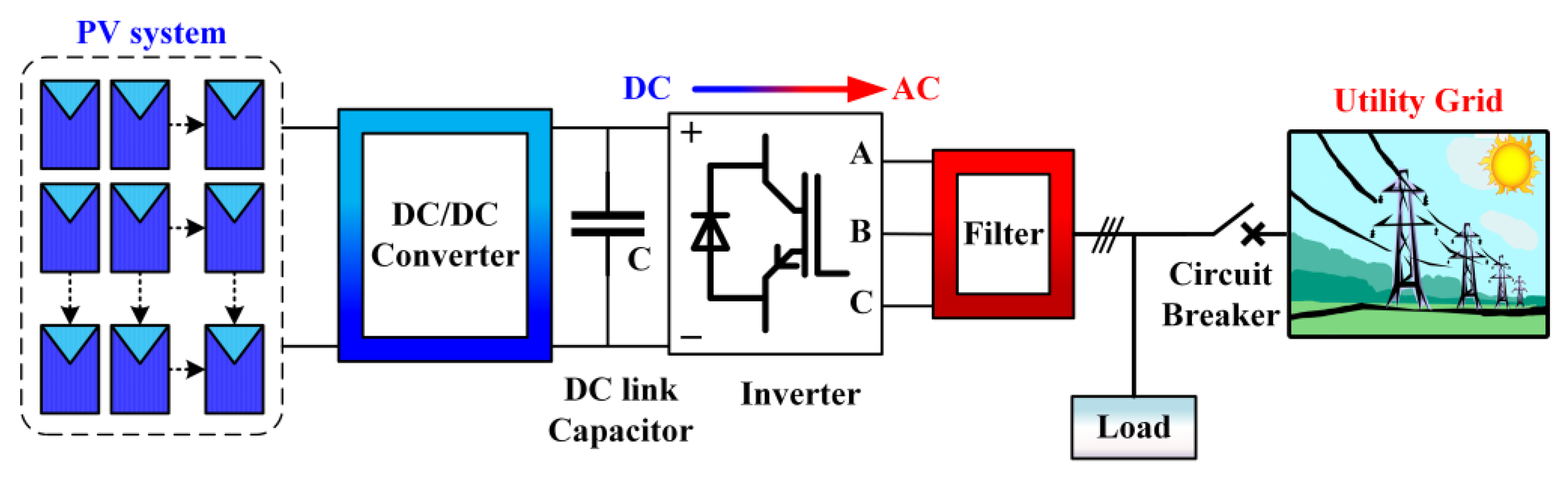
Figure 1. Single-stage PV system.
Energies 16 01492 g001
Figure 2. Dual-stage PV system.
Energies 16 01492 g002
Figure 3. PV network interfaced to three-phase utility grid.
Energies 16 01492 g003
Figure 4. Proposed DC voltage, active and reactive power (DC V-P-Q) control.
Energies 16 01492 g004
Figure 5. Conventional MPPT P&O.
Energies 16 01492 g005
Figure 6. Real power reference generation.
Energies 16 01492 g006
Figure 7. Basic phenomena of particle movement toward the optimal solution.
Energies 16 01492 g007
Figure 8. Sketch map of GBO.
Energies 16 01492 g008
Figure 9. Objective function formulation.
Energies 16 01492 g009
Figure 10. Convergence curve for PSO and GBO.
Energies 16 01492 g010
Figure 11. Tuned DC voltage in grid-connected microgrid.
Energies 16 01492 g011
Figure 12. Tuned active power signal at inverter in grid-connected microgrid.
Energies 16 01492 g012
Figure 13. Tuned active power signal at load in grid-connected microgrid.
Energies 16 01492 g013
Figure 14. Tuned reactive power signal at the inverter in grid-connected microgrid.
Energies 16 01492 g014
Figure 15. Reactive power signal at load in grid-connected microgrid.
Energies 16 01492 g015
Figure 16. THD of line current of tuned grid-interfaced PV after inserting linear load 1.
Energies 16 01492 g016
Figure 17. THD of line current of tuned grid-interfaced PV after inserting nonlinear load.
Energies 16 01492 g017
Figure 18. THD of line current of tuned grid-interfaced PV after inserting linear load 2.
Energies 16 01492 g018
Table 1. Comparison of single-stage and dual-stage grid-tied PV systems.
No.Single StageDual Stage
1Unit control strategy utilized hybrid control of both DC and AC voltage, and injected to DC/AC inverter.DC and AC voltage regulation in
separated parts. DC part injected to DC/DC converter whilst AC part injected to DC/AC inverter.
2Complex, cost effective, high efficiencySimple control, high cost, efficiency degrades
3Bi-directionalBi-directional with extra components
4Component addon depends on power levelComponent addon relies on power level
5Efficiency is higher, especially at rising power levels and densitiesAcceptable efficiency at low to medium power levels and densities
6Output stage more ruggedOutput stage less rugged
Table 2. Simulation parameters for the proposed systems.
Hyper VariablesValue
Root-mean-square voltage ( V r m s ) 240   V
Rated frequency ( f ) 50   Hz
Switching frequency ( f s w ) 10   KHz
DC link voltage ( V D C ) 740
DC link capacitor ( C l i n k ) 30   mF
Inverter choke (RL) of LC filter R = 0.0017   Ω ,   L = 0.54656   mH
Filter (C) parameters ( Q C ,   P C ) of LC filter Q C = 10   Kvar  
P C = Q C × 0.02 = 200   W
Source impedance of the utility grid R = 1   Ω ,   L = 6   mH
Linear load 1 40   KW ,   20   KVar
Linear load 2 40   KW ,   20   KVar
Nonlinear load KW ,   10   KVar
Table 3. Optimized parameters obtained at the end of the simulation.
OptimizationObjective Function K P d K I d K P q K I q Best Fitness Value
Conventional--16.56.5−30.55.5--
PSOITAE31.90843.8527−42.63282.92076.3401
OF17.27077.8545−49.89791.8395783.8754
GBOITAE81.9607411.082475−64.220465.013572.7762
OF53.669024.6988−37.32612.51749413.8754
Table 4. Comparison between controller-based PSO and GBO in terms of transient response.
SubjectStudied ConditionMethodOver-Shoot/Undershoot (%)Peak Time (s)Settling Time (s)
PV
Active Power
Inset of Linear Load 1PSO35.62070.51660.5194
GBO29.81950.51230.5166
Inset of Nonlinear LoadPSO58.96231.52571.5268
GBO57.507321.519611.5207
Inset of Linear Load 2PSO33.85062.58272.6408
GBO31.56342.53742.5709
PV
Reactive Power
Inset of Linear Load 1PSO29.82490.53540.54627
GBO29.53410.531020.5385
Inset of Nonlinear LoadPSO38.85011.53611.5459
GBO37.95561.529681.5456
Inset of Linear Load 2PSO15.14762.52162.6412
GBO13.24632.518602.57921
Disclaimer/Publisher’s Note: The statements, opinions and data contained in all publications are solely those of the individual author(s) and contributor(s) and not of MDPI and/or the editor(s). MDPI and/or the editor(s) disclaim responsibility for any injury to people or property resulting from any ideas, methods, instructions or products referred to in the content.

