Abstract
SMES technology based on MgB superconductor and cryogenic-free cooling can offer a viable solution to power-intensive storage in the short term. One of the main obstacles to the development of dry-cooled SMES systems is the heat load removal due to the AC loss of the superconductor during fast charging and discharging cycles at high power. Accurate knowledge of the amount and distribution of AC loss in the coil is of paramount importance for the sizing and the design of the cooling system and for assessing the possible operational limits of the technology. In this manuscript, the AC loss of a 500 kJ/200 kW multifilamentary MgB SMES during charge–discharge cycling at full power is numerically investigated. The methodology and assumptions of the calculation are briefly resumed, and numerical results are reported and discussed in detail. In particular, the time profile and the distribution of the dissipated power all over the coil are reported. An average dissipation of 85.5 mW/m is found all over the coil during one charge–discharge cycle at full power, with a peak of 150.1 mW/m in the turns lying at the ends of the coil.
1. Introduction
Superconducting magnetic energy storage (SMES) is an established technology based on low-temperature superconductor (LTS) materials. Several LTS SMES systems with rating up to 10 MW have been developed in the past and integrated into the grid [1,2,3,4]. In these systems, the superconductor (Ni-Ti) operates at 4.2 K and the cooling is obtained utilizing a liquid helium (LHe) bath. Despite the technical success, LTS SMES technology has not been widespread in the market due to the complexity, the cost and the safety concerns related to LHe usage. The use of new high-temperature superconductors enables new prospects for SMES technology, today available at the industrial level and able to operate (for the required field level) at much higher temperatures and in the range of 20–50 K compatible with LHe-free cooling [5,6,7,8,9,10,11]. In particular, using MgB with dry cooling offers a viable short-term and low-cost alternative for developing SMES technology [11,12,13,14,15,16,17]. In this context, the national DRYSMES4GRID research project has been funded by the Italian Minister of Economic Development (MISE) and aimed at demonstrating the viability of MgB SMES technology with no use of liquid cryogens [18,19].
One of the main obstacles to the development of dry-cooled SMES systems is the heat load removal due to AC loss of the superconductor during fast charging and discharging cycles at high power. Accurate knowledge of the amount and distribution of AC loss in the coil is of paramount importance for the sizing and the design of the cooling system and for assessing the possible operational limits of the technology, while substantial work has been conducted for predicting AC loss of SMES coils (or fast ramping coils in general) made of 2G HTS tapes (ReBCO coated conductors) [10,20,21,22,23,24], little work has been conducted for calculating the AC loss of SMES coils made of multifilamentary MgB conductors. This paper investigates the space- and time-distribution of AC loss of an MgB SMES coil during rated operation at 200 kW. The coil is made of a composite six-filament MgB tape. We also discuss the cooling requirements for continuous operation (charge–discharge cycling) of the coil at rated power. The analysis was made employing the THELMA code, which is an in-house numerical environment for the coupled thermal-hydraulic (TH) and electromagnetic (EM) analysis of superconductor cables subject to transport current and applied field initially developed for fusion systems [25,26]. The work was carried out in the frame of the DRYSMES4GRID project aimed at developing a dry-cooled MgB SMES system with a rating of 500 kJ/200 kW. A reference six-filament MgB conductor was first selected, and the executive design of the 200 kW coil was carried out [27]. The project was recently concluded with successful results concerning the possibility of fast ramping operation of the dry-cooled MgB coil, thanks to the realization and test of a demonstrator with a 7 kW power rating. This paper focuses on the original full-scale coil with a 200 kW power rating. The details of the scaled-down demonstrator and the testing results will be the subject of a separate publication.
The paper is organized as follows. First, the characteristics of the MgB conductor and the 200 kW SMES coil are resumed in Section 2, along with the considered operating conditions. The THELMA model used to carry out the calculation is briefly resumed in Section 3, along with the main modeling assumptions and parameters as well as the description of the modeled geometry. Numerical results of the space- and time- distribution of the AC loss during SMES operation are reported and discussed in Section 4. Total cooling power is analyzed, and possible operation limits regarding standby time for thermal recovery before the next charge–discharge cycle are also discussed. Concluding remarks are finally drawn in Section 5.
2. Reference MgB Conductor Main Characteristics and Coil Operating Conditions
A composite MgB tape with a 2.05 × 1.1 mm rectangular cross-section was initially selected to develop the 200 kW SMES coil. The tape comprises six MgB filaments embedded in a Nickel matrix and surrounded by a Monel sheath. The filaments are twisted with a 600 mm twist pitch. The filling factor of the superconductor is 29%. The micrography of the described conductor is shown in Table 1. A copper strip with 500 m thickness is co-laminated and tin-soldered onto the tape before electrical insulation to improve the coil’s stability and quench protection. The tape’s critical current is 461 A at 22 K and 1.8 T. The vs. B performance of the tape in the temperature range from 22 K to 30 K is shown in Figure 1. A practically isotropic behavior was observed in all the considered temperature and field ranges with no appreciable impact on the magnetic field direction. The main characteristics of the MgB tape conductor used for the model are resumed in Table 1.

Table 1.
Main characteristics of the MgB conductor.
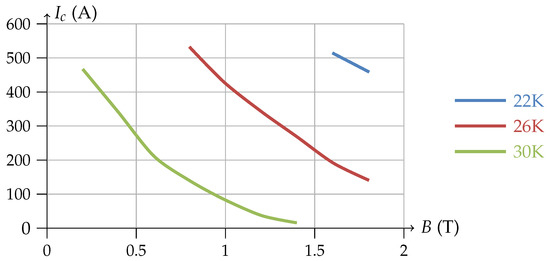
Figure 1.
vs. B performance of the six-filament MgB tape for temperatures of 22 K, 26 K and 30 K.
The dry-cooled MgB coil with 500 kJ deliverable energy and 200 kW power, forming the core of the SMES system, was designed based on the selected tape. The coil is a solenoid with an inductance H, made of 10 layers of 522 turns, each corresponding to a total length of tape of 10.1 km. The main characteristics of the coil are listed in Table 2. The design details, including mechanical, thermal and 3D quench analysis, are reported in [28]. The coil is connected to the three-phase power grid using a DC/DC chopper and a DC/AC inverter connected to a common DC bus, forming the power conditioning systems (PCSs) of the SMES. An operating voltage V is chosen for the DC bus based on the design consideration of the converters. To withstand this voltage and the corresponding electric stress, particularly during the fast commutation of the DC/DC converter, a 125 m thick insulation is applied to the tape through the polyester wrapping. Since a deliverable/absorbed power kW is to be guaranteed, the SMES cannot be discharged below a minimum current A (). Hence, the energy that can be extracted, at a power rate not lower than 200 kW, when the coil operates with a current is given by Equation (1).
Table 2.
Main characteristics of the MgB SMES.
In order to ensure the target deliverable energy of 500 kJ, the operating current of the coil must reach the maximum value A. The total energy stored in the coil at the maximum operating current is 741 kJ. It is pointed out that a residual energy of 241.7 kJ is still stored in the coil when the minimum current of 266.6 A is reached. This energy can still be extracted at a power rate lower than 200 kW and continuously decreases as the discharge proceeds. Hence, similar to all other storage systems, the complete discharge of the SMES cannot be considered for practical applications where a minimum power must be guaranteed for providing the required service.
The temperature T and the coil’s current (via the magnetic field) affect the conductor’s critical current. Hence, a different is obtained depending on the operating conditions. The curves with the designed coil’s constant ratio are shown in Figure 2 as a function of the operating temperature and current. The curves with constant deliverable energy are also shown in the same plot. Since, according to Equation (1), the deliverable energy does not depend on the operating temperature but only on the current, these latter curves appear as horizontal lines in the T vs. plane. A target value of was chosen during the coil design as a compromise between an appropriate safety margin and a reasonable usage of a superconductor. It can be seen from Figure 2 that in order to not exceed the chosen margin of 0.6 in the most severe operating condition, when the SMES is fully charged at 467 A, the operating temperature of the coil must not exceed 16.2 K.
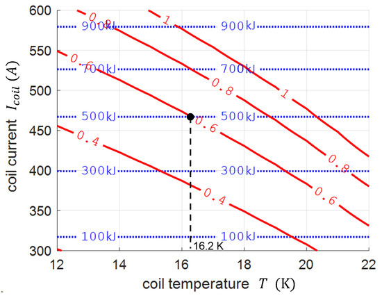
Figure 2.
Performance of the coil as a function of the operating temperature and current. Red lines represent the loci of points with a constant ratio. Dotted horizontal lines represent the deliverable energy corresponding to the operating current.
The total AC loss increases with the ramp rate, hence, with the power delivered or absorbed by the coil. For calculating the AC loss in the most severe conditions, a complete discharge/charge cycle at full power is considered in this paper. The discharge and the charge at 200 kW last 2.5 s, and the cycle lasts 5 s. We now consider a generic time instant , in which the SMES current is , and assume that starting from , the SMES delivers a constant (positive or negative) power P to the grid. By stating the energy balance and neglecting the losses, time evolution of the SMES current is obtained as reported in Equation (2).
Equation (2) is generally valid and holds regardless of the power converters’ architecture and the DC bus’s voltage. In Equation (2), the generator convention is assumed, whereby the coil delivers a positive power and corresponds to a decrease in the SMES current. The time profile of the SMES current during a complete discharge–charge cycle at full power obtained utilizing Equation (2) is shown in Figure 3 and will be used as the input for the AC loss calculation in the following sections.
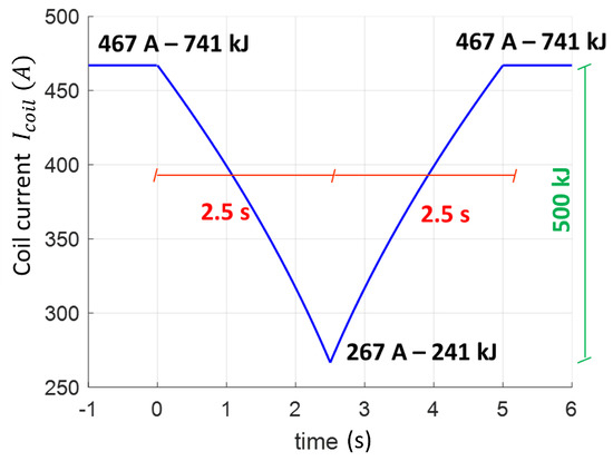
Figure 3.
The current (blue trace) of the SMES coil during one discharge–charge cycle at full power kW.
3. Calculation Model and Simulated Cases
The AC loss of the designed MgB coil during a discharge–charge cycle is calculated employing the electromagnetic module of the THELMA model. This model was initially developed, in cooperation with the Polytechnic University of Turin and the University of Udine, for the coupled thermal–hydraulic (TH) and electromagnetic (EM) analysis of superconductor cables subject to transport current and applied field in the frame of an EFDA initiative aimed at the analysis of fusion systems [28]. The electromagnetic module of the model, developed by the University of Bologna and used in this research [25,26], has been successfully used in a variety of problems involving different materials and architectures, including cable-in-conduit conductor (CICC) [29,30], Rutherford cables [31] and multi-filamentary wires [32]. The main features of the THELMA model are described in this Section. Further information related to the numerical implementation is reported in Appendix A.
3.1. Geometrical Model and Simulated Cases
For calculating the current distribution and AC loss, the MgB conductor forming a specified portion (a set of turns) of the SMES coil is subdivided into a finite number of 3D elements. Only the longitudinal conducting filaments of the conductor (i.e., the six MgB filaments and the copper strip) are considered in this phase. The matrix materials (nickel and Monel) are taken into account using the transverse conductance (as explained in the next Section) and are not directly included in the geometrical model. The 2D model of the conducting elements shown in Figure 4a, comprising elements, is first introduced. The 3D geometrical model, shown in Figure 4b, is generated by the extrusion of the 2D subdivision along the helix pattern of the coil. To account for twisting, a rotation perpendicular to the helix pattern is added to the filaments upon the extrusion. The length of the extrusion step is assigned and is a sub-multiple of the twist pitch so that an entire number of subdivisions is included in one twisting length. The extrusion is continued until the desired length of the conductor to be modeled is reached. In the process, sections, separated by one extrusion length, are introduced. The first and the last of these sections lay on the terminals of the modeled length of the conductor, whereas the remaining lay at the interior. Overall, 3D elements and nodes are generated. These nodes, referred to as primal nodes, correspond to the centers of the faces shared by two longitudinally adjacent elements or laying on the terminal sections of the domain and are used for assembling the solving system of the numerical problem. The interior sections are formed by the faces shared by two adjacent elements and lying at the same position along the axial length of the modeled conductor. Each of the interior sections includes nodes. In this paper, we have modeled ten consecutive turns of conductors, for which the detailed space- and time- distribution of current and AC loss during one discharge and charge cycle is looked for. A uniform current density is assumed in the remaining part of the coil, which acts as a time-varying magnetic field source for the domain under investigation. The ten modeled turns belong to the same layer as shown in Figure 4c and correspond to a total conductor length of about 19 m. A total of six subdivisions per twist pitch were used, corresponding to 190 sections and a total of 1323 3D elements (, , ). The modeled turns can occupy different positions within the coil, giving rise to different AC losses depending on the field condition at the considered position. In this manuscript, we investigated twenty different cases in which the turns were placed at the middle and the bottom of each of the ten layers, as it is schematically shown in Figure 4d for the innermost layer. The AC loss distribution and the overall energy injected in the coil during the discharge–charge cycle are finally obtained based on the results of the individual simulations, and the required cooling power and operation limits are deduced accordingly. A convergence analysis was run to investigate the impact of the number of simulated turns and the number of subdivisions per twist pitch on the numerical results. It was found that no appreciable change was produced in the calculated distributions of current and AC loss by increasing the number of simulated turns and/or by increasing the number of subdivisions per twist pitch. In every longitudinal subdivision of the discretization, each filament (superconductor or copper strip) is modeled by one element only. Hence, the total current of one longitudinal conducting element is uniformly spread all over the cross-section, and no detail of the current distribution can be obtained. Nevertheless, the coupling currents and overall current of SC filaments and strips, as well as their distribution along the conductor’s length, can be correctly reproduced through the model.
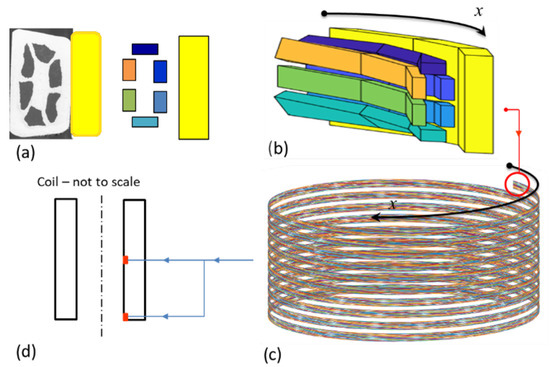
Figure 4.
(a) Micrography and 2D geometrical model of the MgB filaments and the copper strip. (b) 3D geometrical of a short conductor’s length. (c) Geometrical model of 10 turns. (d) Two considered positions (at the middle and the bottom of the innermost layer) of the 10 turns within the coil.
3.2. Mathematical Model
The arc length x of the coil helix, shown in Figure 4b,c, is used to state the problem. At any point of the modeled domain, any information on the discretized domain (axis of elements, vertexes, cross-section and so forth) is deduced from the x coordinate. A uniform current density is assumed in the cross-section of the longitudinal element (superconductor or strip). Any longitudinal element h of the discretization can exchange coupling current in the transverse direction (perpendicular to x) through the matrix material. The current balance of an element with infinitesimal length is schematized in Figure 5, where I is the longitudinal current of the terminal sections of the element and is expressed in A and K is the transversal coupling current per unit length that leaves or enters the element all along the lateral surface and is expressed in A/m. By stating the charge conservation, Equation (3) relation is obtained between the longitudinal current I and the transverse current K per unit length of the element.
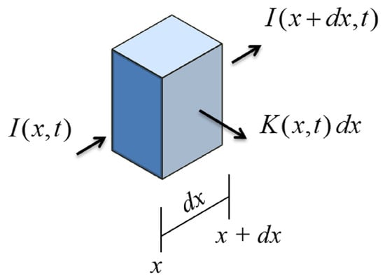
Figure 5.
Current balance of an infinitesimal element.
The electric field at any point of the domain is related to the current density using the constitutive law of the material. The following vs. power law is used for modeling the superconductor material, yielding a nonlinear resistivity
where and n are the critical electric field and the power law exponent, respectively. A liner resistivity is assumed instead for the copper, the Monel and the matrix’s nickel. By using Faraday’s law, the electric field is expressed using the vector magnetic potential and the scalar electric potential v as
where the non-linearity of the resistivity applied to the superconductor is pointed out. In Equation (5), the total magnetic vector potential is split in a contribution due to the longitudinal currents following in the filaments (superconductor or strip), a contribution due to the transverse coupling currents flowing in the matrix and a contribution due to the current circulating in the remaining part of the coil not included in the modeling domain. A solution of the longitudinal current distribution problem is looked for in the weak form by imposing that Equation (5) is satisfied at any of the nodes of the subdivision, supplemented by imposing that the overall current at any cross-section of the conductor coincides with the transport current . In order to account for the coupling currents that develop all over the modeled length, the longitudinal problem is interleaved with the transverse problem, as it is schematized in Figure 6. In particular, it is imposed that Equation (5) is satisfied on the further set of dual nodes obtained by interleaving the original (primal) node. These further nodes are in total () and coincide with the centers of the longitudinal elements. Furthermore, two additional nodes are involved in the model to account for the connection of the modeled domain with the rest of the coil (see Appendix A). It is assumed that the inductive contribution of the transverse currents to the longitudinal and transverse electric fields is negligible. In other words, it is assumed that the time derivative of the vector potential produced by the transverse current is much smaller than the terms and produced by the longitudinal current and the transport current of the coil, respectively. Based on this assumption, Equation (5) yields
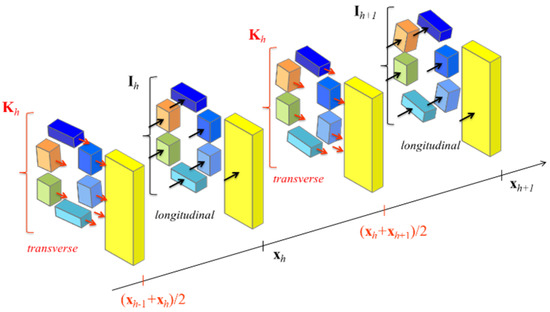
Figure 6.
Representation for the interleaved longitudinal and transverse current distribution problems. Red arrows represent the total transverse current exchanged through the overall lateral surface and can leave (if ) or enter (if ) the element. Black arrows represent the longitudinal currents at terminal sections of the elements and may differ from each other due to the transverse current.
In this way, a non-dynamic circuit is associated with the transverse problem that allows for solving the scalar electric potential v. More in particular, since due to neglecting no time derivative of transverse currents is involved, the scalar electric potential v of all nodes can be related, via the matrix of the mutual conductances between the elements, to the transversal currents and, afterward, to the longitudinal currents via Equation (3). The matrix of conductances needed for solving the transverse problem is calculated using commercial software during pre-processing. In this way, the solving system of the longitudinal problem (Equation (6) at the primal nodes) only involves the time derivative of the longitudinal currents and forms the state equation of the dynamic problem that can be expressed as
in which is the vector of currents in the first () filaments at the internal primal nodes (i.e., not lying on the terminal sections), is the matrix of the mutual inductance coefficients, is the vector of the electromotive forces induced by the time change of the field produced by the coil, is the vector of the resistive voltage drops and vector takes the effect of the applied coil current into account.
Since in the investigated cases, the coil operates in steady state in the initial instant of the simulation, a uniform current in the superconductor filaments and no current in the copper strip is assumed as the initial condition by assigning vector accordingly. The details on the deduction of Equation (7) and the precise definition of the terms involved are reported in Appendix A.
Once the longitudinal currents are obtained, at any instant, by solving the state Equation (7), the transverse current can be obtained by taking the numerical space derivative according to Equation (3). Hence, the profile of current density J can be reconstructed, at any instant, all over the modeled length of the conductor, both in the conducting filaments and in the matrix material. Finally, the distribution of AC loss, in W/m, can be obtained by taking and the overall AC loss, in W, of the modeled domain can be obtained from the volume integral. In particular, the overall loss can be split into the two components and , occurring in the longitudinal filaments (superconductor and Cu strip) and in the matrix, respectively, and calculated as
It is finally stressed that the matrix of the differential Equation (7) is dense and may require prohibitive storage resources and inversion time by increasing the number of elements. A method for replacing Equation (7) with a sparse and, hence, more manageable problem, obtained by involving only the deviation of the elements’ current from the value that it would reach in case of uniform distribution among the filaments, is discussed in Appendix A. In Section 4, the results of the calculation of the AC loss of the MgB coils are reported. The parameters assumed to carry out the calculation are listed in Table 3. In all simulations, isothermal operation at the design value of 16.2 K was assumed.
Table 3.
Parameters used for the numerical calculation.
4. Numerical Results and Discussion
The AC loss of the MgB coil during one complete discharge–charge cycle at full power (200 kW) is calculated in this section. The main loss data obtained are finally summarized in Table 4. The coil’s current during the cycle is shown in Figure 3 and is assigned as the model domain’s transport current in the calculation. The discharge phase starts at when the coil operates at the maximum current A and ends at the time s when it reaches the minimum current A. Afterward, the recharge starts that ends at s when the coil reaches the maximum current again. Strict steady-state operation at constant current is assumed before ( s) and after ( s) the cycle. In the following, different time instants during the discharge, the recharge and the steady state are considered to describe the current’s time behavior and the loss distribution. Superconductor filament currents are denoted from to ; refers to the copper strip one.
Table 4.
Main loss of the SMES coil during one discharge–charge cycle at full power.
In Figure 7, the current of the filaments in ten turns placed at the bottom of the inner layer at s, immediately before the start of the discharge, is shown. All over the length of the conductor forming the turns (about 19 m), the total current of the coil (467 A) is uniformly distributed among the superconductor filaments that carry 77.8 A each. No current circulates in the copper strip. Furthermore, no transverse current circulates in the nickel matrix, creating the coupling of the superconductor filaments in this condition. In Figure 8a, the current distribution in the ten turns at s, when the coil’s current reaches 376.3 A and 35% of the stored energy (200 kJ) is discharged, is shown. In Figure 8b, the detail of the distribution over a conductor length of three twist pitches is shown. During this fast-ramping regime, the current is not uniform. In particular, due to the fast-ramping magnetic field investing the conductor, continuous (along the length) circulation of transverse currents occurs which creates the coupling of the filaments. Due to the high resistivity of the Monel sheath surrounding the superconductor filaments, no substantial current is observed in the copper strip. The distribution is periodical with the twist pitch. The coupling currents can be envisioned as current loops crossing the nickel matrix and reclosing in the superconductor filaments, where they sum or subtract to the transport current. As a result, the filaments experience a continuously changing (along the length) current that goes much beyond the uniform current share (that in this case would be 62.7 A per filament, giving the total transport current of 376.3 A), reaching about 200 A. The current is even reversed in the positions where the loop current subtracts from the transport current reaching A. The same behavior discussed above regarding the discharge is also obtained during the recharge. After the ramping cycle, when the coil’s current reaches the steady state again, the induced electromotive force no longer exists, and the transverse current flowing in the resistive matrix relaxes. The profiles of the filaments’ current gradually return to the uniform distribution holding before the ramping (Figure 7): Figure 9a,b shows the current distribution in the ten turns at s when very substantial relaxation has already occurred and at s when relaxation is practically completed, respectively.
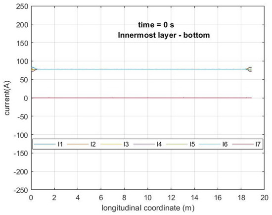
Figure 7.
Current of the filaments in ten turns placed at the bottom of the inner layer at s (before the discharge starts). The total current of the coil is 467A. Currents denoted from to are the currents of the superconductor filaments. Current is the current of the copper strip.
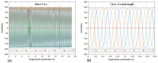
Figure 8.
(a) Current of the filaments in ten turns at s. The total current of the coil is 376.3 A. (b) detail of the current over a conductor length of three twist pitches ( m) at the middle of the ten turns. Currents denoted from to are the currents of the superconductor filaments. Current is the current of the copper strip.
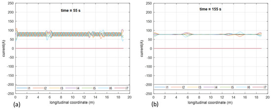
Figure 9.
Current of the filaments in ten turns during steady state after ramping cycle at (a) s and at (b) s. Currents denoted from to are the currents of the superconductor filaments. Current is the current of the copper strip.
As discussed, due to the transverse coupling currents, the current of the filaments goes far beyond the critical value, bringing the superconductor to the dissipative state. This is the main reason for the loss occurring in the conductor. The transverse currents through the resistive nickel matrix also contribute to the total loss, but their impact is much lower. In Figure 10a, the local current of the first filaments () is compared with its critical current () over a conductor length of three twist pitches. The local value of magnetic flux density acting on the conductor () is taken into account for calculating the critical current and is also shown in the figure. The corresponding loss per unit length of the conductor is shown in Figure 10b. It can be seen that the loss in the matrix materials (nickel and Monel sheath) due to transverse current is much lower that the loss in the filaments. It is also pointed out that since negligible current flows in the copper strip and in the Monel matrix, no significant loss is produced therein; thus, practically all of the matrix loss is produced in the nickel.
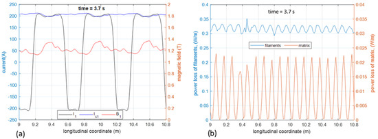
Figure 10.
(a) Current and critical current of filament 1 over a conductor length of three twist pitches at s. The magnetic flux density is also shown in the plot. (b) Total loss per unit length at s in the filaments (superconductor and copper) and in the matrix and sheath materials. Two different scales are used for the filament and the matrix loss.
Figure 11 shows the time profile of loss in a turn at the bottom of the coil during the discharge–charge cycle. It can be seen that the most dissipative phase is at about the middle of the recharge, where a peak power of about 540 mW is reached in the turn. No appreciable dissipation occurs anymore at s, which is one second after the end of the discharge. The conductor’s average dissipation per unit length during the cycle is about 150.1 mW/m, corresponding to 284 mW for the whole turn (1.9 m). Similar power profiles are obtained for the turns in different radial or axial positions along the coil. Figure 12 shows the map of energy loss per unit volume of conductor in one cycle. The data at each point are obtained by taking the time integral of the power of Figure 11 and dividing it by the volume of the conductor (cross-section x length). Linear interpolation in the radial direction and quadratic interpolation in the axial direction were used for obtaining energy loss that was not directly included in the simulations (see Figure 4d and the related discussion in Section 3.1). As expected, higher losses are obtained at the innermost end of the coil due to the higher component of the magnetic field perpendicular to the long side of the conductor. The total loss of the SMES coil in one cycle can be calculated by integrating the distribution of Figure 12; it amounts to 4.32 kJ.
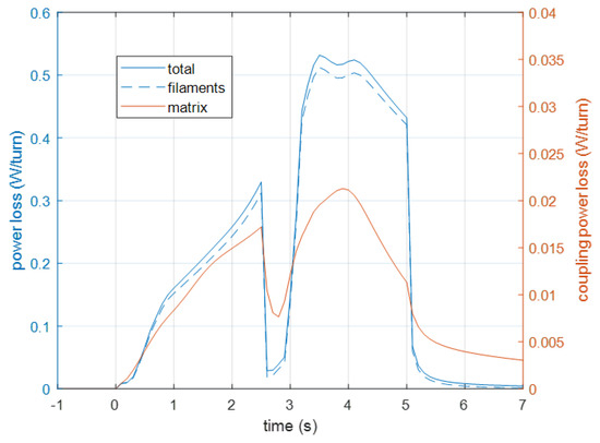
Figure 11.
Total power in the bottom-most turn during the operating cycle. Two different scales are used for the filament and the matrix power.
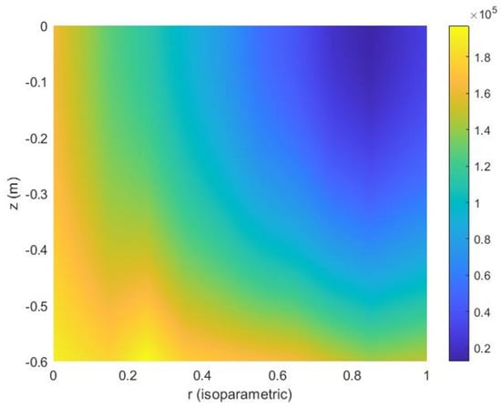
Figure 12.
Map of energy loss per unit volume of conductor (J/m) during one cycle.
5. Conclusions
A method for calculating the AC loss in dynamic conditions of superconducting coils made of multifilamentary MgB tapes with external copper stabilizer was set up. The AC loss of a 500 kJ/200 kW SMES during charge–discharge cycling at full power was numerically investigated by the method. An average dissipation of 85.5 mW/m was found all over the coil during one charge–discharge cycle at full power, with a peak of 150.1 mW/m in the turns lying at the ends of the coil.
Future developments will try to reduce AC losses employing MgB tape or wire with a higher number of filaments (e.g., 19 filaments, currently under development) while at the same time increasing critical current value ( expected).
Author Contributions
A.M., M.F., P.L.R., F.L.F., R.M., U.M., D.M., M.N., A.C., M.T. and C.G. evenly contributed to the manuscript. All authors have read and agreed to the published version of the manuscript.
Funding
This research was funded by Italian Ministry of Economic Development (MISE), Project DRYSMES4GRID, 2017–2021.
Institutional Review Board Statement
Not applicable.
Data Availability Statement
Not applicable.
Conflicts of Interest
The authors declare no conflict of interest.
Appendix A
The details of the THELMA model are described in this section. For simplicity and with no loss of generality, the case of Figure A1, with two filaments () immersed in a conducting matrix, is considered as an example. The filaments are split into four subdivisions, thus generating eight volume elements in total. A set of 10 nodes that correspond to the centers of the faces shared by two longitudinally adjacent elements or laying on the terminal sections of the modeled domain are generated. These nodes are referred to as primal nodes and will be used in the following to obtain the solution to the longitudinal problem. A further set of eight nodes is introduced corresponding to the centers of the volume elements. These nodes are referred to as dual nodes and will be used in the following to relate the solution of the transverse problem to the longitudinal problem. Finally, two more nodes are added for modeling the connection of the modeled domain with a two-terminals component that schematizes the rest of the coil in the considered problem. The coordinate x, schematizing the longitudinal development of the domain, is used to state the problem. The primal nodes lay on the faces separating longitudinally adjacent elements. Hence, sections (or groups) made of primal nodes, each located at the same position along the x coordinate of the modeled domain, can be identified. In the example of Figure A1, five sections of the primal nodes are generated that occupy the positions from to . The dual nodes coincide with the centers of the elements of the subdivision. Similarly, sections (or groups) made of dual nodes, with , each located at the same position along the x coordinate of the modeled domain, can be identified. In Figure A1, the four sections of the dual nodes occupy the positions from to .

Figure A1.
Schematic model of a composite conductor made of two filaments immersed in a conducting matrix. The conductor is supplied with an impressed current . The resistors needed to model the connection at the terminals of the conductor are also included in the model.
Per each filament, any node, both primal and dual, corresponds to a unique value of x. Furthermore, a primal node is adjacent to two dual nodes that precede and follow it, and vice versa. Hence, if a generic quantity q is defined at the dual nodes, its numerical derivative with respect to x is defined at the primal nodes and can be calculated as
where denotes the position of the primal node and and denote the positions of the preceding and following dual nodes within the same filament. Similarly, the numerical derivative at dual node of the quantity q defined in the adjacent primal nodes and is given by
By using Equation (A1) in Equation (3), a linear link is set between the transverse and the longitudinal currents of the filaments, which can be formally expressed by
where is the vector of the transverse currents at the dual section h, and are the vectors of the longitudinal currents at preceding and following primal sections, while and are diagonal matrix operators with dimension , corresponding to the derivative in Equation (A1). Similarly, by using Equation (A1), the projections of the gradients of scalar potential along the filaments’ axis ( indicate the unit vector of the axis) at primal section h can be expressed by
where is the vector of the longitudinal derivatives (gradient’s projections) of the potential at primal section h while and are the vectors of potentials at preceding and following dual sections. is, again, a diagonal matrix operator with dimension .
A solution of the longitudinal problem is now looked for in the weak form. A uniform current density is assumed in the cross-section of the longitudinal element. The magnitude J of the longitudinal component of the current density is obtained as the ratio of the longitudinal current I and the cross-section S of the filament. By imposing that the projection of Equation (6) along the filament axis is satisfied at the j-th node of primal section h not laying on the terminal sections of the domain, we obtain (the dependence of the resistivity on the local current density is implicit)
where is the position of the j-th node of primal section h in the 3D frame. By using Equation (A4), the whole set of in Equation (A5) applied at all nodes of primal section h is rewritten as
where is the whole vector of currents at all primal nodes, is a current-dependent diagonal matrix with k-th term of the diagonal given by the ratio of resistivity and the cross-section and is the vector of the projections, along the axis of the filaments, of the vector potential produced by a unit current in the coil. is the dense, long-range interaction matrix, with dimension representing the effect of the vector potential of all longitudinal currents on the voltage balances of section h and is defined as
In Equation (A7), indicates the volume, spanned by the integration point , of the two consecutive elements of the subdivision that share the primal node k, with k ranging from 1 to . For calculating the coefficient we assume, via the geometric coefficient , that the current density due to unit current at primal node k changes linearly along the axis of the element. It is important to recall that, as discussed in Section 3.2, for obtaining Equation (A5), the time derivative of the vector potential produced by the transverse current was neglected with respect to terms and in the Faraday’s law Equation (5). Consequently, vector of the transverse currents does not appear under the time derivative.
Per each of the primal sections, both laying at the interior or at the terminals of the modeled domain, the sum of the longitudinal currents flowing in the filaments must coincide with the transport current of the coil. Hence, not all of the NF currents of one primal section and the terminal sections are independent since they must have an assigned sum, and an algebraic constraint must then be introduced that can be expressed as
where 1 is a vector made of elements. In total, scalar algebraic equation must be added to the set of matrix Equation (A6).
For solving the transverse problem, we express the transverse current per unit length exchanged between filaments m and n as
where is the conductance per unit length between filaments m and n. By taking the line integral of the approximate Faraday’s law of Equation (6) along a transverse path connecting two dual points, m and n of the same section at position are considered, obtaining
which is rewritten as
where is the line integral of the vector potential produced by a unit current in the coil and coefficient k-th of vector (having terms in total) given by
where the same definitions of the symbols as for Equation (A7) apply. The total transverse current of filament m at the considered position is given by the sum of currents exchanged with all other filaments ( and ) and, by using Equation (A11), is expressed by
having
where is the vector of the potentials of all the dual nodes (equivalently, of all the filaments) of the considered dual section. It is important to point out that, per each of the dual sections, among Equation (A13), only are independent, and one must be disregarded. Without loss of generality, the -th is disregarded in the following. By assembling the independent Equation (A13) for all the dual nodes of the h-th Section at position (except that for the -th one), the following matrix equation is obtained
where is the vector of transverse currents at all dual nodes of the section except the -th, and is the vector of potentials at all dual nodes of the section. Finally, by substituting Equation (A3) in Equation (A15), the following equation is obtained
where and are the vectors of longitudinal currents at all nodes, except the -th one, of the primal sections that precede and follow the dual section h, respectively, and matrices are obtained from matrices in Equation (A3) by suppressing the rows referring to excluded dual nodes. Matrix Equation (A15) is in total as the dual sections relate the potentials of the dual nodes to the currents of the primal nodes. The conductances per unit length needed, starting from Equation (A9) to build Equation (A15), are calculated during the commercial software pre-processing.
Figure A2 shows the model used for calculating the conductance between filament 1 of the MgB conductor and all the others (including the copper strip) as an example. A significant current is exchanged by filament 1 only with the neighboring ones (filaments 2 and 6); hence, negligible conductance is found with respect to the other filaments. In particular, due to the high resistivity of the Monel, a very small conductance is found between all the superconducting filaments and the copper strip. This is behind the negligible current circulating in the copper strip found in Section 4. It is also reported that, due to twisting, the relative position of the filaments within the cross-section changes, thus impacting the conductance value per unit length obtained along one twisting pitch. In Figure A3, the conductance between filament 1 and all others along three twisting pitches is shown. It can be seen that the conductance of filament 1 with respect to the neighboring filaments (2 and 6) changes by about 30% depending on the position along the twisting pitch, following a periodic behavior. Furthermore, the conductance with respect to the other filaments (3, 4, and 5) is two orders of magnitude lower, and the conductance with respect to the copper strip is completely negligible.

Figure A2.
(a) Model for calculating the conductance between filament 1 of the MgB conductor and all the others. (b) Results of voltage and current distribution.

Figure A3.
Conductance per unit length along three twisting pitches for (a) filament 1 and (b) all the others.
Two additional nodes, denoted as and in Figure A1, are added to complete the numerical model. Zero potential is assigned to the additional node , which serves as the reference node. A resistive joint model, assuming that all nodes of the first and the last dual sections are connected, respectively, to the additional nodes and employing an assigned resistance , is used for calculating the potential of the additional nodes at the input and output section, leading to
The overall solving system of the coupled transverse and longitudinal problems is obtained by considering the following items:
- Equation (A6) are applied to all the primal sections not laying on the terminals of the domain. These consist of matrix equations corresponding to scalar equations;
- Equation (A8) for all the longitudinal sections. These consist of scalar equations;
- Equation (A16) applied to all the dual sections. These consist of matrix equation corresponding to scalar equations;
- Terminal conditions in Equation (A17). These consist of 2 matrix equations corresponding to scalar equations.
The solving system of Equation (A18) involves equations in total (we recall that ). The unknowns of the system are:
- longitudinal currents at the primal sections;
- electric scalar potentials of the nodes at the dual sections;
- One electric scalar potentials of node .
leading to a total of .
Equation (A18) forms an algebraic–differential system. For extracting the state equation of the dynamic problem under investigation, the differential part of the system needs to be extracted by algebraic manipulation. Firstly, the scalar potentials at the dual nodes are eliminated by substituting their expression (from Equation (A16)) in all other equations. Then, from terminal conditions of Equation (A17), the currents at the terminal sections are eliminated too. Finally, from Equation (A8), the current of the -th filament at each primal section can be eliminated. A differential solving system consisting of equations is finally obtained, which is expressed as
in which the unknowns , appearing under the time-derivative operator, are the currents in the first filaments at the internal primal nodes (i.e., not lying on the terminal sections).
It is finally reported that the matrix of the differential Equation (A19) is dense and may require prohibitive storage resources and inversion time by increasing the number of elements. To overcome this problem, the current of filament h at primal section k is split into two distinct contributions: a "uniform component", that is, the current which would flow in case of uniform distribution of the total , and a "difference current", which represents the deviation from uniformity, that is
When calculating (via Equations (A7) and (A12)) the mutual induction coefficients between two currents, if the corresponding elements are far enough, the contribution of the deviation current is much smaller than the one of the uniform component and can be neglected. Hence, using this assumption and by substituting Equation (A20) by Equation (A19), the following solving system is obtained
where is the vector of the deviation currents of the filaments at the internal primal nodes, and is now a sparse matrix. In essence, the contribution to of the current of a far element is only considered through the uniform component and is incorporated into vector .
References
- Boenig, H.; Hauer, J. Commissioning tests of the Bonneville Power Administration 30 MJ superconducting magnetic energy storage unit. IEEE Trans. Power Appar. Syst. 1985, 104, 302–312. [Google Scholar] [CrossRef]
- Nagaya, S.; Hirano, N.; Katagiri, T.; Tamada, T.; Shikimachi, K.; Iwatani, Y.; Saito, F.; Ishii, Y. The state of the art of the development of SMES for bridging instantaneous voltage dips in Japan. Cryogenics 2012, 52, 708–712. [Google Scholar] [CrossRef]
- Morandi, A.; Breschi, M.; Fabbri, M.; Negrini, F.; Penco, R.; Perrella, M.; Ribani, P.L.; Tassisto, M.; Trevisani, L. Design, Manufacturing and Preliminary Tests of a Conduction Cooled 200 kJ Nb-Ti μSMES. IEEE Trans. Appl. Supercond. 2008, 18, 697–700. [Google Scholar] [CrossRef]
- Ottonello, L.; Canepa, G.; Albertelli, P.; Picco, E.; Florio, A.; Masciarelli, G.; Rossi, S.; Martini, L.; Pincella, C.; Mariscotti, A.; et al. The largest italian SMES. IEEE Trans. Appl. Supercond. 2006, 16, 602–607. [Google Scholar] [CrossRef]
- Tixador, P.; Bellin, B.; Deleglise, M.; Vallier, J.C.; Bruzek, C.; Allais, A.; Saugrain, J. Design and first tests of a 800 kJ HTS SMES. IEEE Trans. Appl. Supercond. 2007, 17, 1967–1972. [Google Scholar] [CrossRef]
- Lee, S.; Yi, K.P.; Park, S.H.; Lee, J.K.; Kim, W.S.; Park, C.; Bae, J.H.; Seong, K.C.; Park, I.; Choi, K.; et al. Design of HTS toroidal magnets for a 5 MJ SMES. IEEE Trans. Appl. Supercond. 2011, 22, 5700904. [Google Scholar]
- Shikimachi, K.; Hirano, N.; Nagaya, S.; Kawashima, H.; Higashikawa, K.; Nakamura, T. System coordination of 2 GJ class YBCO SMES for power system control. IEEE Trans. Appl. Supercond. 2009, 19, 2012–2018. [Google Scholar] [CrossRef]
- Song, M.; Shi, J.; Liu, Y.; Xu, Y.; Hu, N.; Tang, Y.; Ren, L.; Li, J. 100 kJ/50 kW HTS SMES for micro-grid. IEEE Trans. Appl. Supercond. 2014, 25, 5700506. [Google Scholar] [CrossRef]
- Xu, Y.; Tang, Y.; Ren, L.; Dai, Q.; Xu, C.; Wang, Z.; Shi, J.; Li, J.; Liang, S.; Yan, S. Numerical simulation and experimental validation of a cooling process in a 150-kJ SMES magnet. IEEE Trans. Appl. Supercond. 2016, 26, 5700507. [Google Scholar] [CrossRef]
- Morandi, A.; Fabbri, M.; Gholizad, B.; Grilli, F.; Sirois, F.; Zermeño, V.M. Design and comparison of a 1-MW/5-s HTS SMES with toroidal and solenoidal geometry. IEEE Trans. Appl. Supercond. 2016, 26, 5700606. [Google Scholar] [CrossRef]
- Morandi, A.; Gholizad, B.; Fabbri, M. Design and performance of a 1 MW-5 s high temperature superconductor magnetic energy storage system. Supercond. Sci. Technol. 2015, 29, 015014. [Google Scholar] [CrossRef]
- Saichi, Y.; Miyagi, D.; Tsuda, M. A suitable design method of SMES coil for reducing superconducting wire usage considering maximum magnetic flux density. IEEE Trans. Appl. Supercond. 2013, 24, 5700505. [Google Scholar] [CrossRef]
- Sander, M.; Gehring, R.; Neumann, H. LIQHYSMES—A 48 GJ toroidal MgB2-SMES for buffering minute and second fluctuations. IEEE Trans. Appl. Supercond. 2012, 23, 5700505. [Google Scholar] [CrossRef]
- Shintomi, T.; Asami, T.; Suzuki, G.; Ota, N.; Takao, T.; Makida, Y.; Hamajima, T.; Tsuda, M.; Miyagi, D.; Kajiwara, M.; et al. Design Study of MgB2 SMES Coil for Effective Use of Renewable Energy. IEEE Trans. Appl. Supercond. 2012, 23, 5700304. [Google Scholar] [CrossRef]
- Leys, P.; Klaeser, M.; Ruf, C.; Schneider, T. Characterization of Commercial MgB 2 conductors for magnet application in SMES. IEEE Trans. Appl. Supercond. 2016, 26, 6200605. [Google Scholar] [CrossRef]
- Morandi, A.; Fiorillo, A.; Pullano, S.; Ribani, P.L. Development of a small cryogen-free MgB 2 test coil for SMES application. IEEE Trans. Appl. Supercond. 2017, 27, 5700404. [Google Scholar] [CrossRef]
- Tran, V.T.; Islam, M.R.; Muttaqi, K.M.; Sutanto, D. A novel application of magnesium di-boride superconducting energy storage to mitigate the power fluctuations of single-phase PV systems. IEEE Trans. Appl. Supercond. 2019, 29, 5700505. [Google Scholar] [CrossRef]
- Morandi, A.; Anemona, A.; Angeli, G.; Breschi, M.; Della Corte, A.; Ferdeghini, C.; Gandolfi, C.; Grandi, G.; Grasso, G.; Martini, L.; et al. The DRYSMES4GRID project: Development of a 500 kJ/200 kW cryogen-free cooled SMES demonstrator based on MgB2. IEEE Trans. Appl. Supercond. 2018, 28, 5700205. [Google Scholar] [CrossRef]
- Gandolfi, C.; Chiumeo, R.; Raggini, D.; Faranda, R.; Morandi, A.; Ferdeghini, C.; Tropeano, M.; Turtù, S. Study of a Universal Power SMES Compensator for LV Distribution Grid. In Proceedings of the 2018 AEIT International Annual Conference, Bari, Italy, 3–5 October 2018; pp. 1–6. [Google Scholar]
- Park, M.J.; Kwak, S.Y.; Kim, W.S.; Lee, S.W.; Lee, J.K.; Han, J.H.; Choi, K.D.; Jung, H.K.; Seong, K.C.; Hahn, S.y. AC loss and thermal stability of HTS model coils for a 600 kJ SMES. IEEE Trans. Appl. Supercond. 2007, 17, 2418–2421. [Google Scholar] [CrossRef]
- Wang, Z.; Tang, Y.; Ren, L.; Li, J.; Xu, Y.; Liao, Y.; Deng, X. AC loss analysis of a hybrid HTS magnet for SMES based on H-formulation. IEEE Trans. Appl. Supercond. 2016, 27, 4701005. [Google Scholar]
- Zhang, Z. AC Loss Database Built with Numerical Multi-scale Model and Status Prediction of a 150 kJ SMES. In Proceedings of the 2018 IEEE International Magnetics Conference (INTERMAG), Singapore, 23–27 April 2018; p. 1. [Google Scholar]
- Zhang, Z.; Ren, L.; Xu, Y.; Wang, Z.; Xia, Y.; Liang, S.; Yan, S.; Tang, Y. AC loss prediction model of a 150 kJ HTS SMES based on multi-scale model and artificial neural networks. IEEE Trans. Magn. 2018, 54, 7206005. [Google Scholar] [CrossRef]
- Chen, Y.; Chen, X.Y.; Zeng, L.; Xie, Q.; Lei, Y. AC loss and temperature simulations of HTS pancake coil during SMES operations. In Proceedings of the 2020 IEEE International Conference on Applied Superconductivity and Electromagnetic Devices (ASEMD), Tianjin, China, 16–18 October 2020; pp. 1–2. [Google Scholar]
- Ciotti, M.; Nijhuis, A.; Ribani, P.; Richard, L.S.; Zanino, R. THELMA code electromagnetic model of ITER superconducting cables and application to the ENEA stability experiment. Supercond. Sci. Technol. 2006, 19, 987. [Google Scholar] [CrossRef]
- Breschi, M.; Ribani, P.L. Electromagnetic modeling of the jacket in cable-in-conduit conductors. IEEE Trans. Appl. Supercond. 2008, 18, 18–28. [Google Scholar] [CrossRef]
- Fabbri, M.; Grandi, G.; Morandi, A.; Melaccio, U.; Ribani, P.L. Design of the magnet system. In Deliverable D01 of Funded Project DRYSEMS4GRID, MISE—Italian Ministry of Economic Development, Competitive Call “Research Project for Electric Power Grid”, 2017–2021; University of Bologna: Bologna, Italy, 2021. (In Italian) [Google Scholar]
- Bellina, F.; Bonicelli, T.; Breschi, M.; Ciotti, M.; Della Corte, A.; Formisano, A.; Ilyin, Y.; Marchese, V.; Martone, R.; Nijhuis, A.; et al. Superconductive cables current distribution analysis. Fusion Eng. Des. 2003, 66, 1159–1163. [Google Scholar] [CrossRef]
- Breschi, M.; Ribani, P.L.; Bellina, F. Electromagnetic analysis of the voltage-temperature characteristics of the ITER TF conductor samples. IEEE Trans. Appl. Supercond. 2009, 19, 1512–1515. [Google Scholar] [CrossRef]
- Manfreda, G.; Bellina, F.; Corato, V.; della Corte, A.; Ribani, P. Coupled thermal and electromagnetic analysis of the NAFASSY magnet. IEEE Trans. Appl. Supercond. 2014, 25, 4801406. [Google Scholar] [CrossRef]
- Breschi, M.; Cavallucci, L.; Ribani, P.; Calzolaio, C.; Sanfilippo, S. Analysis of losses in superconducting magnets based on the Nb3Sn Rutherford cable configuration for future gantries. Supercond. Sci. Technol. 2017, 31, 015005. [Google Scholar] [CrossRef]
- Breschi, M.; Ribani, P.L.; Scurti, F.; Nijhuis, A.; Bajas, H.; Devred, A. Electromechanical Modeling of Nb3Sn Superconducting Wires Subjected to Periodic Bending Strain. IEEE Trans. Appl. Supercond. 2014, 25, 1–5. [Google Scholar] [CrossRef]

Disclaimer/Publisher’s Note: The statements, opinions and data contained in all publications are solely those of the individual author(s) and contributor(s) and not of MDPI and/or the editor(s). MDPI and/or the editor(s) disclaim responsibility for any injury to people or property resulting from any ideas, methods, instructions or products referred to in the content. |
© 2023 by the authors. Licensee MDPI, Basel, Switzerland. This article is an open access article distributed under the terms and conditions of the Creative Commons Attribution (CC BY) license (https://creativecommons.org/licenses/by/4.0/).