
Research on the Optimal Design of Seasonal Time-of-Use Tariff Based on the Price Elasticity of Electricity Demand

Abstract
:
1. Introduction
1.1. Background and Motivation
1.2. Literature Review and Contribution
- (1)
- The traditional PEED matrix is mostly constructed as (3 × 3), including three stages of peak-flat, flat-valley, and peak-valley. Such a simple matrix may lead to an inaccurate calculation of load fluctuation in each period, which will lead to unreasonable TOU pricing.
- (2)
- Not all users are aware of their PEED and DR abilities, so the method of determining PEED based on a questionnaire in the existing literature is not universal. Meanwhile, direct setting of PEED based on expert experience also has strong subjectivity.
- (3)
- At present, most of the existing studies are based on the original set of TOU tariffs to optimize a new set of TOU tariffs, which means the designed tariff is the same in each month/season. However, as mentioned above, power users have different electricity consumption characteristics in different seasons, and electricity price optimization in a single season is not universal.
- (1)
- The clustering of a typical day’s load curve based on the K-means++ algorithm is first adopted in this paper, which is proven to have better clustering performance than the traditional methods.
- (2)
- Compared with the traditional (3 × 3) matrix, the (24 × 24) PEED matrix established in this paper is more comprehensive. In addition, the PEED coefficient is calculated based on the actual load data, which is more accurate than questionnaires or direct settings in the existing studies.
- (3)
- The seasonal characteristics are incorporated into the traditional TOU tariff optimization design model. Through this study, the optimal TOU tariff for four seasons can be obtained instead of one, which is more practical and universal.
2. Methodology
2.1. K-Means++ Algorithm
- ➢
- Step 1: Select objects from the load data as the initial cluster center .
- ➢
- Step 2: Calculate the Euclidean distance from each cluster object to the cluster center.
- ➢
- Step 3: Recalculate each cluster center.
- ➢
- Step 4: Repeat Step 1 and Step 2 until the position of the cluster center does not change anymore.
- ➢
- Step 5: Take one center , chosen uniformly at random from .
- ➢
- Step 6: Calculate the shortest distance between each sample and the existing cluster center. Then, calculate the probability that each sample point is selected as the next cluster center, and select the sample point corresponding to the maximum probability value as the next cluster center. The probability can be expressed as follows:
- ➢
- Step 7: Repeat Step 6 until cluster centers are obtained.
2.2. Price Elasticity of Electricity Demand Model
3. TOU Tariff Optimization Model based on the PEED
3.1. Objective Function
3.2. Constraints
- ➢
- Consumer electricity cost constraint.
- ➢
- Peak-valley tariff constraints.
- ➢
- Power consumption balance constraint.
4. Case Study
4.1. Data Sources
4.2. Clustering of Typical Daily Load Curves in Four Seasons based on K-Means++ Algorithm
4.3. TOU Tariff Optimization Results Analysis
- (1)
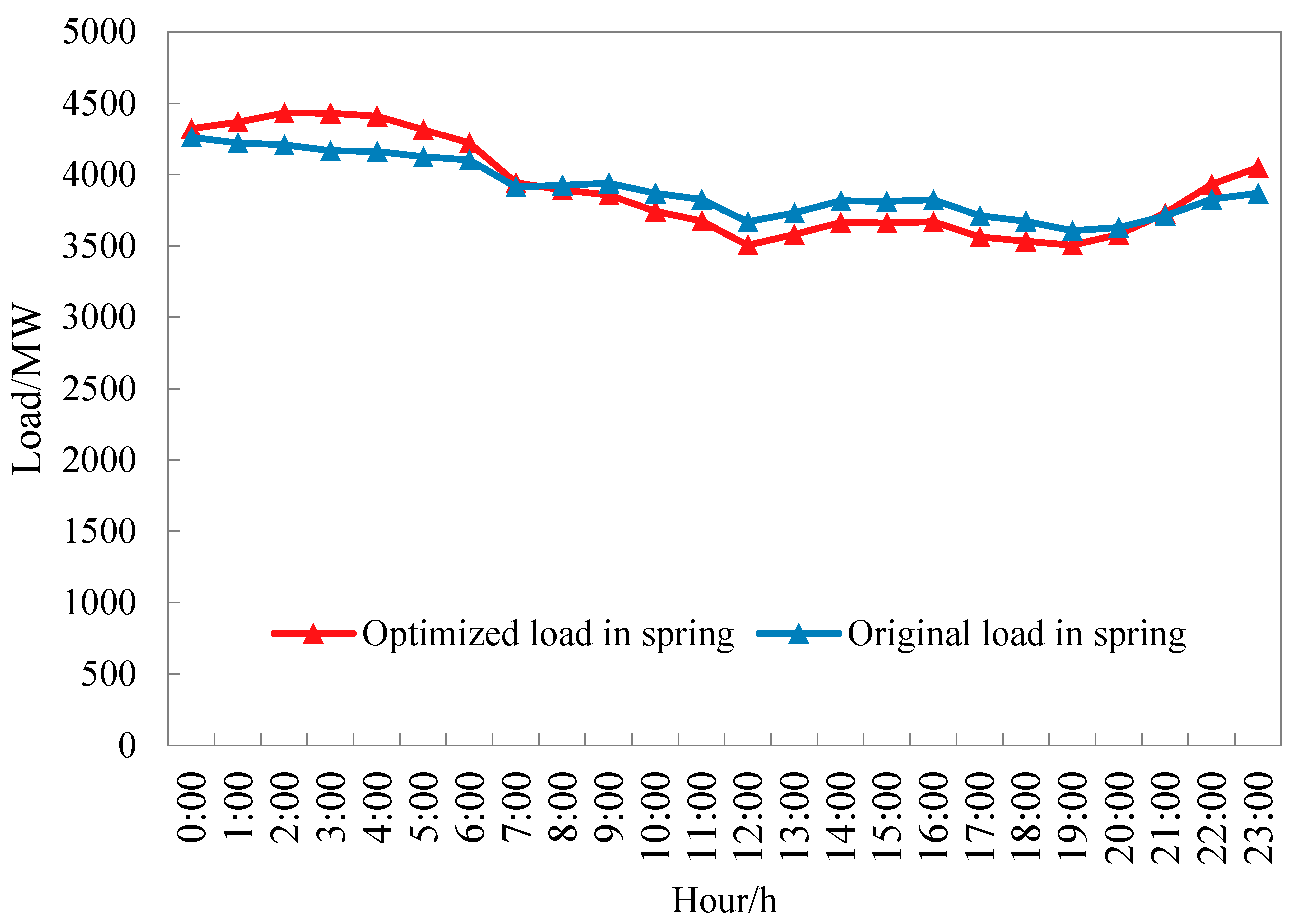
- Optimization results for TOU tariffs in spring.
- (2)
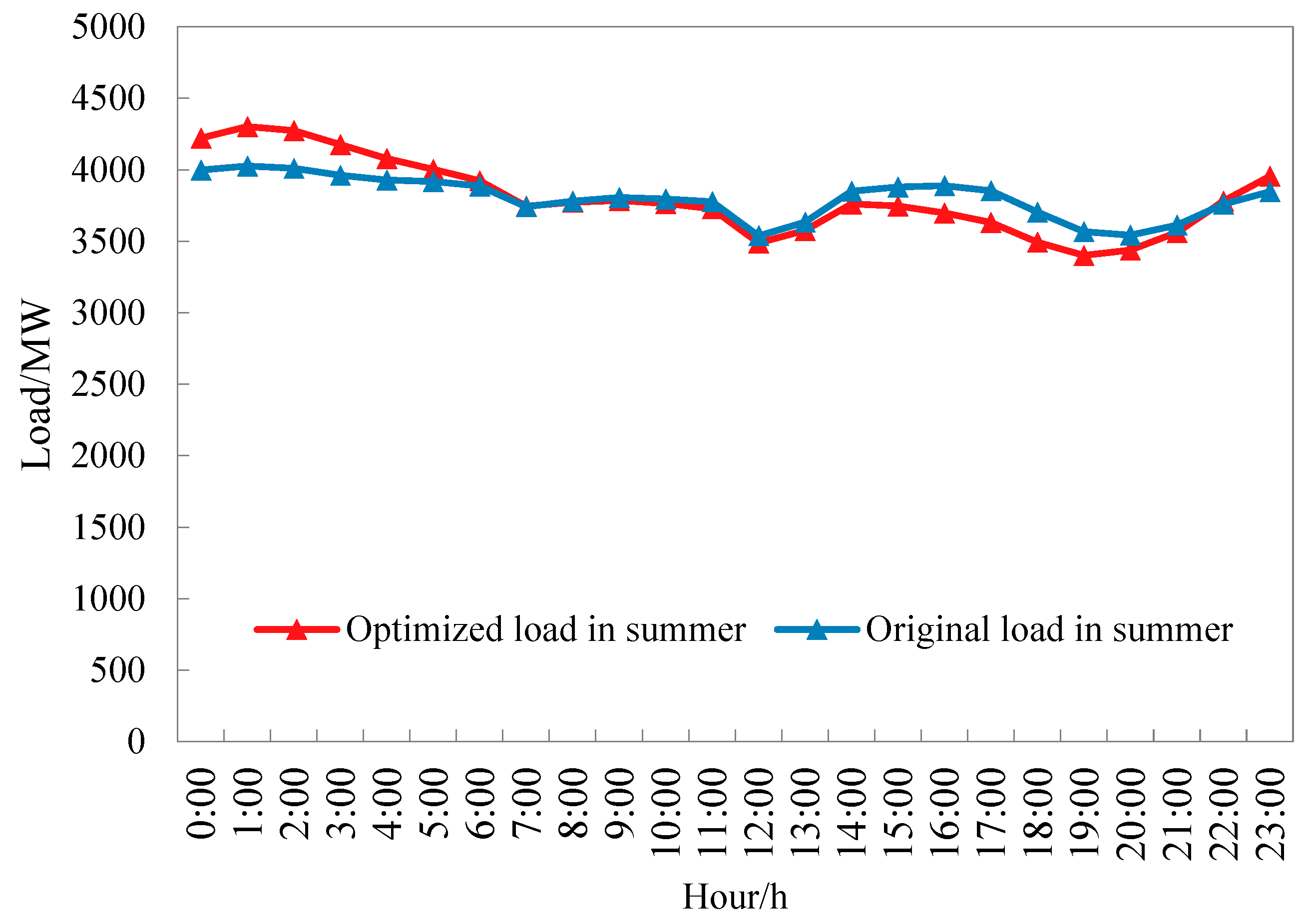
- Optimization results for TOU tariffs in summer.
- (3)
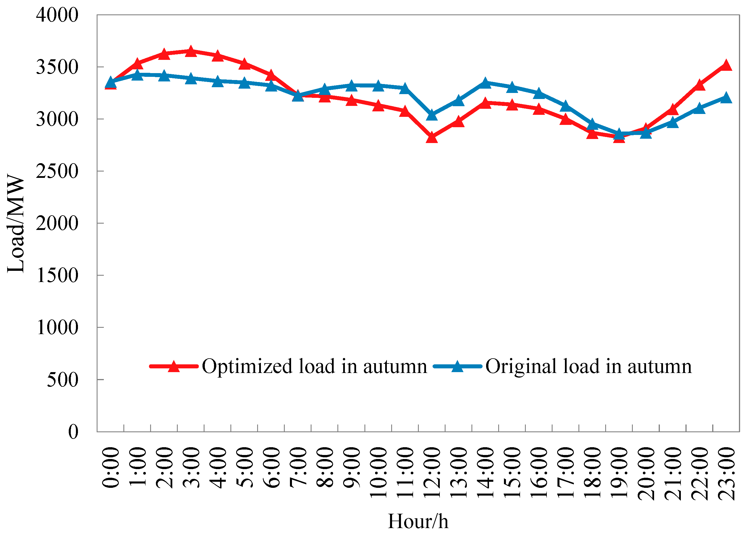
- Optimization results for TOU tariffs in autumn.
- (4)
- Optimization results for TOU tariff in winter.
- (5)
- Discussion of TOU tariff optimization results.
4.4. Comparison Results
5. Conclusions and Suggestions
5.1. Conclusions
- (1)
- Compared with the traditional K-means algorithm, the K-means++ algorithm used in this paper has a better clustering effect. The typical daily load curve of four seasons obtained through K-means++ clustering is more scientific and reasonable.
- (2)
- To improve the accuracy of the PEED matrix, this paper expands the original (3 × 3) matrix to the (24 × 24) matrix. The results show that the elastic coefficients (including self-elastic and cross-elastic) at different times are not the same, even within the same period. A more accurate and comprehensive PEED matrix is significant for the rational design of the TOU tariff.
- (3)
- The seasonal TOU tariff optimization model constructed in this paper obtains the TOU tariff and typical daily load curve in four seasons. Compared with the original TOU tariff, the optimized seasonal TOU tariff increases by 8.06–15.39% in the peak period and decreases by 18.48–27.95% in the valley period. The TOU tariff optimization also results in a decrease of 4.03–8.02% of the load in the peak period and an increase of 6.41–9.75% of the load in the valley period.
- (4)
- Compared with the traditional TOU optimization models, the proposed model can increase the peak-valley load difference by 7.70% and reduce the power consumption cost by 1.36%.
5.2. Limitations and Future Outlook
- (1)
- From the perspective of methodology, although the model proposed in this paper has excellent effects, it is easy to understand how it could lead to problems such as low computational efficiency and long computation times.
- (2)
- Due to the data constraints, this paper only conducts TOU tariff optimization design for the industrial sector, and the empirical object only comes from the actual data of one province in China.
- (1)
- In the future, we will evaluate the electricity consumption habits and laws of power users in different regions and industries so as to calculate a more abundant PEED coefficient.
- (2)
- In the future, we will further expand the data samples to different sectors in more provinces, making the optimized TOU tariff more universal and practical.
Author Contributions
Funding
Data Availability Statement
Acknowledgments
Conflicts of Interest
Abbreviations
| Abbreviation | Full Name |
| DSM | demand side management |
| DLC | direct load control |
| DSB | demand side bidding |
| EDR | emergency demand response |
| ASM | ancillary service market |
| DR | demand response |
| TOU | time-of-use |
| RTP | real-time price |
| CPP | critical peak price |
| NDRC | National Development and Reform Commission |
| PFV | peak-flat-valley |
| IFCM | improved fuzzy C-means clustering |
| PEED | price elasticity of electricity demand |
| SSE | sum of squared errors |
Appendix A

| 0:00 | 1:00 | 2:00 | 3:00 | 4:00 | 5:00 | 6:00 | 7:00 | 8:00 | 9:00 | 10:00 | 11:00 | 12:00 | 13:00 | 14:00 | 15:00 | 16:00 | 17:00 | 18:00 | 19:00 | 20:00 | 21:00 | 22:00 | 23:00 | |
|---|---|---|---|---|---|---|---|---|---|---|---|---|---|---|---|---|---|---|---|---|---|---|---|---|
| 0:00 | −0.038 | −0.038 | −0.024 | −0.009 | 0.010 | 0.024 | 0.028 | 0.031 | 0.036 | 0.034 | 0.030 | 0.023 | 0.009 | 0.001 | 0.002 | 0.012 | 0.024 | 0.025 | 0.017 | −0.007 | −0.037 | −0.051 | −0.056 | −0.047 |
| 1:00 | −0.038 | −0.037 | −0.038 | −0.023 | −0.008 | 0.010 | 0.024 | 0.028 | 0.031 | 0.036 | 0.035 | 0.030 | 0.023 | 0.008 | 0.001 | 0.001 | 0.012 | 0.023 | 0.025 | 0.017 | −0.007 | −0.037 | −0.051 | −0.055 |
| 2:00 | −0.024 | −0.038 | −0.037 | −0.038 | −0.024 | −0.009 | 0.010 | 0.024 | 0.027 | 0.031 | 0.036 | 0.035 | 0.030 | 0.023 | 0.008 | 0.001 | 0.001 | 0.012 | 0.024 | 0.025 | 0.017 | −0.007 | −0.036 | −0.051 |
| 3:00 | −0.009 | −0.023 | −0.038 | −0.038 | −0.039 | −0.024 | −0.009 | 0.010 | 0.024 | 0.027 | 0.032 | 0.036 | 0.035 | 0.030 | 0.023 | 0.008 | 0.001 | 0.001 | 0.012 | 0.024 | 0.025 | 0.017 | −0.007 | −0.036 |
| 4:00 | 0.010 | −0.008 | −0.024 | −0.039 | −0.038 | −0.039 | −0.024 | −0.009 | 0.010 | 0.024 | 0.028 | 0.032 | 0.036 | 0.035 | 0.030 | 0.023 | 0.008 | 0.001 | 0.002 | 0.013 | 0.024 | 0.025 | 0.017 | −0.007 |
| 5:00 | 0.024 | 0.010 | −0.009 | −0.024 | −0.039 | −0.038 | −0.039 | −0.024 | −0.009 | 0.010 | 0.024 | 0.028 | 0.032 | 0.036 | 0.035 | 0.030 | 0.023 | 0.008 | 0.001 | 0.002 | 0.013 | 0.024 | 0.025 | 0.017 |
| 6:00 | 0.028 | 0.024 | 0.010 | −0.009 | −0.024 | −0.039 | −0.038 | −0.039 | −0.024 | −0.009 | 0.010 | 0.024 | 0.028 | 0.032 | 0.036 | 0.035 | 0.030 | 0.023 | 0.009 | 0.002 | 0.002 | 0.013 | 0.024 | 0.025 |
| 7:00 | 0.031 | 0.028 | 0.024 | 0.010 | −0.009 | −0.024 | −0.039 | −0.038 | −0.039 | −0.024 | −0.009 | 0.010 | 0.024 | 0.028 | 0.032 | 0.036 | 0.035 | 0.030 | 0.024 | 0.009 | 0.002 | 0.002 | 0.013 | 0.024 |
| 8:00 | 0.036 | 0.031 | 0.027 | 0.024 | 0.010 | −0.009 | −0.024 | −0.039 | −0.039 | −0.039 | −0.024 | −0.009 | 0.010 | 0.024 | 0.028 | 0.032 | 0.036 | 0.035 | 0.030 | 0.024 | 0.009 | 0.002 | 0.002 | 0.013 |
| 9:00 | 0.034 | 0.036 | 0.031 | 0.027 | 0.024 | 0.010 | −0.009 | −0.024 | −0.039 | −0.038 | −0.039 | −0.024 | −0.009 | 0.010 | 0.024 | 0.028 | 0.032 | 0.036 | 0.035 | 0.030 | 0.024 | 0.009 | 0.002 | 0.002 |
| 10:00 | 0.030 | 0.035 | 0.036 | 0.032 | 0.028 | 0.024 | 0.010 | −0.009 | −0.024 | −0.039 | −0.038 | −0.039 | −0.024 | −0.009 | 0.010 | 0.024 | 0.028 | 0.032 | 0.036 | 0.035 | 0.030 | 0.024 | 0.009 | 0.002 |
| 11:00 | 0.023 | 0.030 | 0.035 | 0.036 | 0.032 | 0.028 | 0.024 | 0.010 | −0.009 | −0.024 | −0.039 | −0.038 | −0.039 | −0.024 | −0.009 | 0.010 | 0.024 | 0.028 | 0.032 | 0.036 | 0.035 | 0.030 | 0.024 | 0.009 |
| 12:00 | 0.009 | 0.023 | 0.030 | 0.035 | 0.036 | 0.032 | 0.028 | 0.024 | 0.010 | −0.009 | −0.024 | −0.039 | −0.038 | −0.039 | −0.024 | −0.009 | 0.010 | 0.024 | 0.028 | 0.032 | 0.036 | 0.035 | 0.030 | 0.024 |
| 13:00 | 0.001 | 0.008 | 0.023 | 0.030 | 0.035 | 0.036 | 0.032 | 0.028 | 0.024 | 0.010 | −0.009 | −0.024 | −0.039 | −0.038 | −0.039 | −0.024 | −0.009 | 0.010 | 0.024 | 0.028 | 0.032 | 0.036 | 0.035 | 0.030 |
| 14:00 | 0.002 | 0.001 | 0.008 | 0.023 | 0.030 | 0.035 | 0.036 | 0.032 | 0.028 | 0.024 | 0.010 | −0.009 | −0.024 | −0.039 | −0.038 | −0.039 | −0.024 | −0.009 | 0.010 | 0.024 | 0.028 | 0.032 | 0.036 | 0.035 |
| 15:00 | 0.012 | 0.001 | 0.001 | 0.008 | 0.023 | 0.030 | 0.035 | 0.036 | 0.032 | 0.028 | 0.024 | 0.010 | −0.009 | −0.024 | −0.039 | −0.038 | −0.039 | −0.024 | −0.009 | 0.010 | 0.024 | 0.028 | 0.032 | 0.036 |
| 16:00 | 0.024 | 0.012 | 0.001 | 0.001 | 0.008 | 0.023 | 0.030 | 0.035 | 0.036 | 0.032 | 0.028 | 0.024 | 0.010 | −0.009 | −0.024 | −0.039 | −0.038 | −0.039 | −0.024 | −0.009 | 0.010 | 0.024 | 0.028 | 0.032 |
| 17:00 | 0.025 | 0.023 | 0.012 | 0.001 | 0.001 | 0.008 | 0.023 | 0.030 | 0.035 | 0.036 | 0.032 | 0.028 | 0.024 | 0.010 | −0.009 | −0.024 | −0.039 | −0.038 | −0.039 | −0.024 | −0.009 | 0.010 | 0.024 | 0.028 |
| 18:00 | 0.017 | 0.025 | 0.024 | 0.012 | 0.002 | 0.001 | 0.009 | 0.024 | 0.030 | 0.035 | 0.036 | 0.032 | 0.028 | 0.024 | 0.010 | −0.009 | −0.024 | −0.039 | −0.039 | −0.039 | −0.024 | −0.009 | 0.010 | 0.024 |
| 19:00 | −0.007 | 0.017 | 0.025 | 0.024 | 0.013 | 0.002 | 0.002 | 0.009 | 0.024 | 0.030 | 0.035 | 0.036 | 0.032 | 0.028 | 0.024 | 0.010 | −0.009 | −0.024 | −0.039 | −0.039 | −0.039 | −0.024 | −0.009 | 0.010 |
| 20:00 | −0.037 | −0.007 | 0.017 | 0.025 | 0.024 | 0.013 | 0.002 | 0.002 | 0.009 | 0.024 | 0.030 | 0.035 | 0.036 | 0.032 | 0.028 | 0.024 | 0.010 | −0.009 | −0.024 | −0.039 | −0.039 | −0.039 | −0.024 | −0.009 |
| 21:00 | −0.051 | −0.037 | −0.007 | 0.017 | 0.025 | 0.024 | 0.013 | 0.002 | 0.002 | 0.009 | 0.024 | 0.030 | 0.035 | 0.036 | 0.032 | 0.028 | 0.024 | 0.010 | −0.009 | −0.024 | −0.039 | −0.038 | −0.039 | −0.024 |
| 22:00 | −0.056 | −0.051 | −0.036 | −0.007 | 0.017 | 0.025 | 0.024 | 0.013 | 0.002 | 0.002 | 0.009 | 0.024 | 0.030 | 0.035 | 0.036 | 0.032 | 0.028 | 0.024 | 0.010 | −0.009 | −0.024 | −0.039 | −0.038 | −0.039 |
| 23:00 | −0.047 | −0.055 | −0.051 | −0.036 | −0.007 | 0.017 | 0.025 | 0.024 | 0.013 | 0.002 | 0.002 | 0.009 | 0.024 | 0.030 | 0.035 | 0.036 | 0.032 | 0.028 | 0.024 | 0.010 | −0.009 | −0.024 | −0.039 | −0.038 |
| 0:00 | 1:00 | 2:00 | 3:00 | 4:00 | 5:00 | 6:00 | 7:00 | 8:00 | 9:00 | 10:00 | 11:00 | 12:00 | 13:00 | 14:00 | 15:00 | 16:00 | 17:00 | 18:00 | 19:00 | 20:00 | 21:00 | 22:00 | 23:00 | |
|---|---|---|---|---|---|---|---|---|---|---|---|---|---|---|---|---|---|---|---|---|---|---|---|---|
| 0:00 | −0.035 | −0.039 | −0.027 | −0.016 | −0.001 | 0.008 | 0.009 | 0.013 | 0.019 | 0.022 | 0.023 | 0.020 | 0.010 | 0.008 | 0.015 | 0.031 | 0.043 | 0.042 | 0.028 | −0.001 | −0.033 | −0.047 | −0.050 | −0.041 |
| 1:00 | −0.039 | −0.035 | −0.038 | −0.027 | −0.016 | −0.001 | 0.008 | 0.009 | 0.013 | 0.019 | 0.022 | 0.023 | 0.020 | 0.011 | 0.008 | 0.015 | 0.031 | 0.043 | 0.042 | 0.028 | −0.002 | −0.033 | −0.047 | −0.050 |
| 2:00 | −0.027 | −0.038 | −0.035 | −0.038 | −0.027 | −0.015 | −0.001 | 0.009 | 0.009 | 0.013 | 0.019 | 0.022 | 0.023 | 0.020 | 0.010 | 0.008 | 0.015 | 0.030 | 0.043 | 0.041 | 0.027 | −0.002 | −0.033 | −0.047 |
| 3:00 | −0.016 | −0.027 | −0.038 | −0.034 | −0.038 | −0.027 | −0.015 | 0.000 | 0.009 | 0.009 | 0.012 | 0.019 | 0.022 | 0.023 | 0.020 | 0.010 | 0.008 | 0.015 | 0.030 | 0.042 | 0.041 | 0.027 | −0.002 | −0.033 |
| 4:00 | −0.001 | −0.016 | −0.027 | −0.038 | −0.034 | −0.038 | −0.026 | −0.015 | 0.000 | 0.009 | 0.009 | 0.012 | 0.019 | 0.022 | 0.023 | 0.020 | 0.010 | 0.008 | 0.014 | 0.030 | 0.042 | 0.041 | 0.027 | −0.002 |
| 5:00 | 0.008 | −0.001 | −0.015 | −0.027 | −0.038 | −0.034 | −0.038 | −0.026 | −0.015 | 0.000 | 0.008 | 0.009 | 0.012 | 0.019 | 0.022 | 0.023 | 0.020 | 0.010 | 0.007 | 0.014 | 0.030 | 0.042 | 0.041 | 0.027 |
| 6:00 | 0.009 | 0.008 | −0.001 | −0.015 | −0.026 | −0.038 | −0.034 | −0.037 | −0.026 | −0.015 | −0.001 | 0.008 | 0.009 | 0.012 | 0.019 | 0.022 | 0.023 | 0.020 | 0.010 | 0.007 | 0.014 | 0.030 | 0.042 | 0.041 |
| 7:00 | 0.013 | 0.009 | 0.009 | 0.000 | −0.015 | −0.026 | −0.037 | −0.034 | −0.037 | −0.026 | −0.015 | −0.001 | 0.008 | 0.009 | 0.012 | 0.019 | 0.022 | 0.022 | 0.020 | 0.010 | 0.007 | 0.014 | 0.030 | 0.042 |
| 8:00 | 0.019 | 0.013 | 0.009 | 0.009 | 0.000 | −0.015 | −0.026 | −0.037 | −0.033 | −0.037 | −0.026 | −0.015 | −0.001 | 0.008 | 0.009 | 0.012 | 0.019 | 0.022 | 0.022 | 0.020 | 0.010 | 0.007 | 0.014 | 0.030 |
| 9:00 | 0.022 | 0.019 | 0.013 | 0.009 | 0.009 | 0.000 | −0.015 | −0.026 | −0.037 | −0.034 | −0.038 | −0.027 | −0.015 | −0.001 | 0.008 | 0.009 | 0.012 | 0.018 | 0.021 | 0.022 | 0.020 | 0.009 | 0.007 | 0.014 |
| 10:00 | 0.023 | 0.022 | 0.019 | 0.012 | 0.009 | 0.008 | −0.001 | −0.015 | −0.026 | −0.038 | −0.034 | −0.038 | −0.027 | −0.015 | −0.001 | 0.008 | 0.008 | 0.012 | 0.018 | 0.021 | 0.022 | 0.019 | 0.009 | 0.007 |
| 11:00 | 0.020 | 0.023 | 0.022 | 0.019 | 0.012 | 0.009 | 0.008 | −0.001 | −0.015 | −0.027 | −0.038 | −0.034 | −0.038 | −0.026 | −0.015 | −0.001 | 0.008 | 0.008 | 0.012 | 0.018 | 0.021 | 0.022 | 0.019 | 0.009 |
| 12:00 | 0.010 | 0.020 | 0.023 | 0.022 | 0.019 | 0.012 | 0.009 | 0.008 | −0.001 | −0.015 | −0.027 | −0.038 | −0.034 | −0.038 | −0.026 | −0.015 | −0.001 | 0.008 | 0.008 | 0.012 | 0.018 | 0.021 | 0.022 | 0.019 |
| 13:00 | 0.008 | 0.011 | 0.020 | 0.023 | 0.022 | 0.019 | 0.012 | 0.009 | 0.008 | −0.001 | −0.015 | −0.026 | −0.038 | −0.034 | −0.038 | −0.027 | −0.016 | −0.001 | 0.008 | 0.008 | 0.012 | 0.018 | 0.021 | 0.022 |
| 14:00 | 0.015 | 0.008 | 0.010 | 0.020 | 0.023 | 0.022 | 0.019 | 0.012 | 0.009 | 0.008 | −0.001 | −0.015 | −0.026 | −0.038 | −0.034 | −0.038 | −0.027 | −0.016 | −0.001 | 0.008 | 0.008 | 0.011 | 0.018 | 0.021 |
| 15:00 | 0.031 | 0.015 | 0.008 | 0.010 | 0.020 | 0.023 | 0.022 | 0.019 | 0.012 | 0.009 | 0.008 | −0.001 | −0.015 | −0.027 | −0.038 | −0.034 | −0.038 | −0.027 | −0.016 | −0.001 | 0.007 | 0.008 | 0.011 | 0.018 |
| 16:00 | 0.043 | 0.031 | 0.015 | 0.008 | 0.010 | 0.020 | 0.023 | 0.022 | 0.019 | 0.012 | 0.008 | 0.008 | −0.001 | −0.016 | −0.027 | −0.038 | −0.034 | −0.038 | −0.027 | −0.016 | −0.002 | 0.007 | 0.008 | 0.011 |
| 17:00 | 0.042 | 0.043 | 0.030 | 0.015 | 0.008 | 0.010 | 0.020 | 0.022 | 0.022 | 0.018 | 0.012 | 0.008 | 0.008 | −0.001 | −0.016 | −0.027 | −0.038 | −0.034 | −0.038 | −0.027 | −0.016 | −0.002 | 0.007 | 0.008 |
| 18:00 | 0.028 | 0.042 | 0.043 | 0.030 | 0.014 | 0.007 | 0.010 | 0.020 | 0.022 | 0.021 | 0.018 | 0.012 | 0.008 | 0.008 | −0.001 | −0.016 | −0.027 | −0.038 | −0.034 | −0.038 | −0.027 | −0.016 | −0.002 | 0.007 |
| 19:00 | −0.001 | 0.028 | 0.041 | 0.042 | 0.030 | 0.014 | 0.007 | 0.010 | 0.020 | 0.022 | 0.021 | 0.018 | 0.012 | 0.008 | 0.008 | −0.001 | −0.016 | −0.027 | −0.038 | −0.034 | −0.038 | −0.027 | −0.016 | −0.002 |
| 20:00 | −0.033 | −0.002 | 0.027 | 0.041 | 0.042 | 0.030 | 0.014 | 0.007 | 0.010 | 0.020 | 0.022 | 0.021 | 0.018 | 0.012 | 0.008 | 0.007 | −0.002 | −0.016 | −0.027 | −0.038 | −0.035 | −0.038 | −0.027 | −0.016 |
| 21:00 | −0.047 | −0.033 | −0.002 | 0.027 | 0.041 | 0.042 | 0.030 | 0.014 | 0.007 | 0.009 | 0.019 | 0.022 | 0.021 | 0.018 | 0.011 | 0.008 | 0.007 | −0.002 | −0.016 | −0.027 | −0.038 | −0.035 | −0.039 | −0.027 |
| 22:00 | −0.050 | −0.047 | −0.033 | −0.002 | 0.027 | 0.041 | 0.042 | 0.030 | 0.014 | 0.007 | 0.009 | 0.019 | 0.022 | 0.021 | 0.018 | 0.011 | 0.008 | 0.007 | −0.002 | −0.016 | −0.027 | −0.039 | −0.035 | −0.039 |
| 23:00 | −0.041 | −0.050 | −0.047 | −0.033 | −0.002 | 0.027 | 0.041 | 0.042 | 0.030 | 0.014 | 0.007 | 0.009 | 0.019 | 0.022 | 0.021 | 0.018 | 0.011 | 0.008 | 0.007 | −0.002 | −0.016 | −0.027 | −0.039 | −0.035 |
| 0:00 | 1:00 | 2:00 | 3:00 | 4:00 | 5:00 | 6:00 | 7:00 | 8:00 | 9:00 | 10:00 | 11:00 | 12:00 | 13:00 | 14:00 | 15:00 | 16:00 | 17:00 | 18:00 | 19:00 | 20:00 | 21:00 | 22:00 | 23:00 | |
|---|---|---|---|---|---|---|---|---|---|---|---|---|---|---|---|---|---|---|---|---|---|---|---|---|
| 0:00 | −0.053 | −0.049 | −0.027 | −0.004 | 0.025 | 0.048 | 0.057 | 0.063 | 0.065 | 0.061 | 0.050 | 0.039 | 0.017 | 0.001 | −0.005 | 0.001 | 0.012 | 0.014 | 0.005 | −0.024 | −0.062 | −0.080 | −0.084 | −0.070 |
| 1:00 | −0.049 | −0.053 | −0.049 | −0.028 | −0.004 | 0.025 | 0.048 | 0.057 | 0.063 | 0.065 | 0.061 | 0.050 | 0.039 | 0.017 | 0.001 | −0.005 | 0.001 | 0.012 | 0.014 | 0.005 | −0.024 | −0.062 | −0.080 | −0.084 |
| 2:00 | −0.027 | −0.049 | −0.053 | −0.049 | −0.028 | −0.004 | 0.025 | 0.048 | 0.057 | 0.063 | 0.065 | 0.061 | 0.050 | 0.039 | 0.017 | 0.001 | −0.005 | 0.001 | 0.012 | 0.015 | 0.005 | −0.024 | −0.062 | −0.080 |
| 3:00 | −0.004 | −0.028 | −0.049 | −0.053 | −0.049 | −0.028 | −0.004 | 0.025 | 0.048 | 0.057 | 0.063 | 0.065 | 0.061 | 0.050 | 0.039 | 0.017 | 0.001 | −0.005 | 0.001 | 0.012 | 0.015 | 0.006 | −0.024 | −0.062 |
| 4:00 | 0.025 | −0.004 | −0.028 | −0.049 | −0.053 | −0.049 | −0.028 | −0.004 | 0.024 | 0.048 | 0.057 | 0.063 | 0.065 | 0.061 | 0.050 | 0.039 | 0.017 | 0.001 | −0.005 | 0.001 | 0.013 | 0.015 | 0.006 | −0.024 |
| 5:00 | 0.048 | 0.025 | −0.004 | −0.028 | −0.049 | −0.054 | −0.049 | −0.028 | −0.005 | 0.025 | 0.048 | 0.057 | 0.063 | 0.065 | 0.061 | 0.050 | 0.039 | 0.018 | 0.001 | −0.005 | 0.001 | 0.013 | 0.015 | 0.006 |
| 6:00 | 0.057 | 0.048 | 0.025 | −0.004 | −0.028 | −0.049 | −0.054 | −0.049 | −0.028 | −0.004 | 0.025 | 0.048 | 0.057 | 0.063 | 0.065 | 0.061 | 0.051 | 0.039 | 0.018 | 0.001 | −0.005 | 0.001 | 0.013 | 0.015 |
| 7:00 | 0.063 | 0.057 | 0.048 | 0.025 | −0.004 | −0.028 | −0.049 | −0.054 | −0.049 | −0.028 | −0.004 | 0.025 | 0.048 | 0.057 | 0.063 | 0.065 | 0.061 | 0.051 | 0.039 | 0.018 | 0.001 | −0.005 | 0.001 | 0.013 |
| 8:00 | 0.065 | 0.063 | 0.057 | 0.048 | 0.024 | −0.005 | −0.028 | −0.049 | −0.054 | −0.049 | −0.028 | −0.004 | 0.025 | 0.048 | 0.057 | 0.063 | 0.065 | 0.061 | 0.051 | 0.039 | 0.018 | 0.002 | −0.005 | 0.001 |
| 9:00 | 0.061 | 0.065 | 0.063 | 0.057 | 0.048 | 0.025 | −0.004 | −0.028 | −0.049 | −0.054 | −0.049 | −0.028 | −0.004 | 0.025 | 0.048 | 0.057 | 0.063 | 0.065 | 0.061 | 0.051 | 0.039 | 0.018 | 0.002 | −0.005 |
| 10:00 | 0.050 | 0.061 | 0.065 | 0.063 | 0.057 | 0.048 | 0.025 | −0.004 | −0.028 | −0.049 | −0.054 | −0.049 | −0.028 | −0.004 | 0.025 | 0.048 | 0.057 | 0.063 | 0.066 | 0.061 | 0.051 | 0.040 | 0.018 | 0.002 |
| 11:00 | 0.039 | 0.050 | 0.061 | 0.065 | 0.063 | 0.057 | 0.048 | 0.025 | −0.004 | −0.028 | −0.049 | −0.053 | −0.049 | −0.028 | −0.004 | 0.025 | 0.048 | 0.058 | 0.064 | 0.066 | 0.061 | 0.051 | 0.040 | 0.018 |
| 12:00 | 0.017 | 0.039 | 0.050 | 0.061 | 0.065 | 0.063 | 0.057 | 0.048 | 0.025 | −0.004 | −0.028 | −0.049 | −0.053 | −0.049 | −0.028 | −0.004 | 0.025 | 0.048 | 0.058 | 0.064 | 0.066 | 0.061 | 0.051 | 0.040 |
| 13:00 | 0.001 | 0.017 | 0.039 | 0.050 | 0.061 | 0.065 | 0.063 | 0.057 | 0.048 | 0.025 | −0.004 | −0.028 | −0.049 | −0.054 | −0.049 | −0.028 | −0.004 | 0.025 | 0.048 | 0.058 | 0.064 | 0.066 | 0.061 | 0.051 |
| 14:00 | −0.005 | 0.001 | 0.017 | 0.039 | 0.050 | 0.061 | 0.065 | 0.063 | 0.057 | 0.048 | 0.025 | −0.004 | −0.028 | −0.049 | −0.053 | −0.049 | −0.028 | −0.004 | 0.025 | 0.048 | 0.058 | 0.064 | 0.066 | 0.061 |
| 15:00 | 0.001 | −0.005 | 0.001 | 0.017 | 0.039 | 0.050 | 0.061 | 0.065 | 0.063 | 0.057 | 0.048 | 0.025 | −0.004 | −0.028 | −0.049 | −0.053 | −0.049 | −0.027 | −0.004 | 0.025 | 0.048 | 0.058 | 0.064 | 0.066 |
| 16:00 | 0.012 | 0.001 | −0.005 | 0.001 | 0.017 | 0.039 | 0.051 | 0.061 | 0.065 | 0.063 | 0.057 | 0.048 | 0.025 | −0.004 | −0.028 | −0.049 | −0.053 | −0.049 | −0.027 | −0.004 | 0.025 | 0.048 | 0.058 | 0.064 |
| 17:00 | 0.014 | 0.012 | 0.001 | −0.005 | 0.001 | 0.018 | 0.039 | 0.051 | 0.061 | 0.065 | 0.063 | 0.058 | 0.048 | 0.025 | −0.004 | −0.027 | −0.049 | −0.053 | −0.049 | −0.027 | −0.004 | 0.025 | 0.048 | 0.058 |
| 18:00 | 0.005 | 0.014 | 0.012 | 0.001 | −0.005 | 0.001 | 0.018 | 0.039 | 0.051 | 0.061 | 0.066 | 0.064 | 0.058 | 0.048 | 0.025 | −0.004 | −0.027 | −0.049 | −0.053 | −0.049 | −0.027 | −0.004 | 0.025 | 0.048 |
| 19:00 | −0.024 | 0.005 | 0.015 | 0.012 | 0.001 | −0.005 | 0.001 | 0.018 | 0.039 | 0.051 | 0.061 | 0.066 | 0.064 | 0.058 | 0.048 | 0.025 | −0.004 | −0.027 | −0.049 | −0.053 | −0.049 | −0.027 | −0.004 | 0.025 |
| 20:00 | −0.062 | −0.024 | 0.005 | 0.015 | 0.013 | 0.001 | −0.005 | 0.001 | 0.018 | 0.039 | 0.051 | 0.061 | 0.066 | 0.064 | 0.058 | 0.048 | 0.025 | −0.004 | −0.027 | −0.049 | −0.053 | −0.049 | −0.027 | −0.004 |
| 21:00 | −0.080 | −0.062 | −0.024 | 0.006 | 0.015 | 0.013 | 0.001 | −0.005 | 0.002 | 0.018 | 0.040 | 0.051 | 0.061 | 0.066 | 0.064 | 0.058 | 0.048 | 0.025 | −0.004 | −0.027 | −0.049 | −0.053 | −0.049 | −0.027 |
| 22:00 | −0.084 | −0.080 | −0.062 | −0.024 | 0.006 | 0.015 | 0.013 | 0.001 | −0.005 | 0.002 | 0.018 | 0.040 | 0.051 | 0.061 | 0.066 | 0.064 | 0.058 | 0.048 | 0.025 | −0.004 | −0.027 | −0.049 | −0.053 | −0.049 |
| 23:00 | −0.070 | −0.084 | −0.080 | −0.062 | −0.024 | 0.006 | 0.015 | 0.013 | 0.001 | −0.005 | 0.002 | 0.018 | 0.040 | 0.051 | 0.061 | 0.066 | 0.064 | 0.058 | 0.048 | 0.025 | −0.004 | −0.027 | −0.049 | −0.053 |
| 0:00 | 1:00 | 2:00 | 3:00 | 4:00 | 5:00 | 6:00 | 7:00 | 8:00 | 9:00 | 10:00 | 11:00 | 12:00 | 13:00 | 14:00 | 15:00 | 16:00 | 17:00 | 18:00 | 19:00 | 20:00 | 21:00 | 22:00 | 23:00 | |
|---|---|---|---|---|---|---|---|---|---|---|---|---|---|---|---|---|---|---|---|---|---|---|---|---|
| 0:00 | −0.033 | −0.037 | −0.020 | −0.001 | 0.027 | 0.052 | 0.058 | 0.063 | 0.064 | 0.058 | 0.045 | 0.027 | 0.000 | −0.018 | −0.024 | −0.016 | 0.002 | 0.007 | 0.002 | −0.021 | −0.055 | −0.065 | −0.065 | −0.048 |
| 1:00 | −0.037 | −0.032 | −0.035 | −0.019 | 0.000 | 0.028 | 0.053 | 0.059 | 0.065 | 0.063 | 0.057 | 0.043 | 0.026 | 0.002 | −0.019 | −0.024 | −0.017 | 0.001 | 0.006 | 0.000 | −0.022 | −0.056 | −0.066 | −0.065 |
| 2:00 | −0.020 | −0.035 | −0.030 | −0.034 | −0.017 | 0.002 | 0.030 | 0.055 | 0.061 | 0.063 | 0.061 | 0.055 | 0.043 | 0.028 | 0.001 | −0.019 | −0.025 | −0.018 | −0.001 | 0.004 | −0.001 | −0.024 | −0.057 | −0.066 |
| 3:00 | −0.001 | −0.019 | −0.034 | −0.030 | −0.034 | −0.017 | 0.002 | 0.030 | 0.055 | 0.061 | 0.063 | 0.061 | 0.055 | 0.043 | 0.028 | 0.001 | −0.019 | −0.026 | −0.019 | −0.001 | 0.004 | −0.002 | −0.024 | −0.057 |
| 4:00 | 0.027 | 0.000 | −0.017 | −0.034 | −0.029 | −0.033 | −0.016 | 0.003 | 0.031 | 0.054 | 0.060 | 0.062 | 0.060 | 0.056 | 0.043 | 0.027 | 0.000 | −0.020 | −0.027 | −0.020 | −0.002 | 0.003 | −0.002 | −0.024 |
| 5:00 | 0.052 | 0.028 | 0.002 | −0.017 | −0.033 | −0.029 | −0.032 | −0.016 | 0.004 | 0.031 | 0.054 | 0.059 | 0.062 | 0.061 | 0.056 | 0.043 | 0.027 | 0.000 | −0.021 | −0.027 | −0.020 | −0.003 | 0.003 | −0.002 |
| 6:00 | 0.058 | 0.053 | 0.030 | 0.002 | −0.016 | −0.032 | −0.028 | −0.032 | −0.015 | 0.003 | 0.030 | 0.053 | 0.059 | 0.062 | 0.061 | 0.056 | 0.043 | 0.027 | −0.001 | −0.021 | −0.028 | −0.021 | −0.003 | 0.003 |
| 7:00 | 0.063 | 0.059 | 0.055 | 0.030 | 0.003 | −0.016 | −0.032 | −0.028 | −0.031 | −0.016 | 0.003 | 0.030 | 0.053 | 0.059 | 0.062 | 0.061 | 0.055 | 0.042 | 0.026 | −0.001 | −0.022 | −0.028 | −0.021 | −0.003 |
| 8:00 | 0.064 | 0.065 | 0.061 | 0.055 | 0.031 | 0.004 | −0.015 | −0.031 | −0.029 | −0.030 | −0.015 | 0.004 | 0.030 | 0.052 | 0.060 | 0.062 | 0.062 | 0.056 | 0.043 | 0.027 | 0.000 | −0.021 | −0.028 | −0.020 |
| 9:00 | 0.058 | 0.063 | 0.063 | 0.061 | 0.054 | 0.031 | 0.003 | −0.016 | −0.030 | −0.028 | −0.030 | −0.014 | 0.004 | 0.030 | 0.052 | 0.060 | 0.063 | 0.062 | 0.057 | 0.044 | 0.028 | 0.000 | −0.021 | −0.028 |
| 10:00 | 0.045 | 0.057 | 0.061 | 0.063 | 0.060 | 0.054 | 0.030 | 0.003 | −0.015 | −0.030 | −0.026 | −0.028 | −0.014 | 0.002 | 0.030 | 0.053 | 0.062 | 0.065 | 0.064 | 0.059 | 0.046 | 0.030 | 0.001 | −0.020 |
| 11:00 | 0.027 | 0.043 | 0.055 | 0.061 | 0.062 | 0.059 | 0.053 | 0.030 | 0.004 | −0.014 | −0.028 | −0.026 | −0.028 | −0.014 | 0.002 | 0.030 | 0.054 | 0.062 | 0.065 | 0.065 | 0.060 | 0.047 | 0.030 | 0.001 |
| 12:00 | 0.000 | 0.026 | 0.043 | 0.055 | 0.060 | 0.062 | 0.059 | 0.053 | 0.030 | 0.004 | −0.014 | −0.028 | −0.025 | −0.028 | −0.014 | 0.002 | 0.031 | 0.055 | 0.063 | 0.066 | 0.066 | 0.060 | 0.047 | 0.030 |
| 13:00 | −0.018 | 0.002 | 0.028 | 0.043 | 0.056 | 0.061 | 0.062 | 0.059 | 0.052 | 0.030 | 0.002 | −0.014 | −0.028 | −0.025 | −0.028 | −0.014 | 0.002 | 0.031 | 0.054 | 0.063 | 0.066 | 0.065 | 0.060 | 0.047 |
| 14:00 | −0.024 | −0.019 | 0.001 | 0.028 | 0.043 | 0.056 | 0.061 | 0.062 | 0.060 | 0.052 | 0.030 | 0.002 | −0.014 | −0.028 | −0.025 | −0.028 | −0.013 | 0.004 | 0.032 | 0.056 | 0.065 | 0.068 | 0.066 | 0.061 |
| 15:00 | −0.016 | −0.024 | −0.019 | 0.001 | 0.027 | 0.043 | 0.056 | 0.061 | 0.062 | 0.060 | 0.053 | 0.030 | 0.002 | −0.014 | −0.028 | −0.025 | −0.027 | −0.012 | 0.005 | 0.034 | 0.057 | 0.066 | 0.068 | 0.066 |
| 16:00 | 0.002 | −0.017 | −0.025 | −0.019 | 0.000 | 0.027 | 0.043 | 0.055 | 0.062 | 0.063 | 0.062 | 0.054 | 0.031 | 0.002 | −0.013 | −0.027 | −0.022 | −0.025 | −0.009 | 0.007 | 0.036 | 0.059 | 0.066 | 0.068 |
| 17:00 | 0.007 | 0.001 | −0.018 | −0.026 | −0.020 | 0.000 | 0.027 | 0.042 | 0.056 | 0.062 | 0.065 | 0.062 | 0.055 | 0.031 | 0.004 | −0.012 | −0.025 | −0.020 | −0.023 | −0.007 | 0.009 | 0.038 | 0.060 | 0.067 |
| 18:00 | 0.002 | 0.006 | −0.001 | −0.019 | −0.027 | −0.021 | −0.001 | 0.026 | 0.043 | 0.057 | 0.064 | 0.065 | 0.063 | 0.054 | 0.032 | 0.005 | −0.009 | −0.023 | −0.018 | −0.020 | −0.005 | 0.012 | 0.039 | 0.060 |
| 19:00 | −0.021 | 0.000 | 0.004 | −0.001 | −0.020 | −0.027 | −0.021 | −0.001 | 0.027 | 0.044 | 0.059 | 0.065 | 0.066 | 0.063 | 0.056 | 0.034 | 0.007 | −0.007 | −0.020 | −0.016 | −0.018 | −0.003 | 0.012 | 0.039 |
| 20:00 | −0.055 | −0.022 | −0.001 | 0.004 | −0.002 | −0.020 | −0.028 | −0.022 | 0.000 | 0.028 | 0.046 | 0.060 | 0.066 | 0.066 | 0.065 | 0.057 | 0.036 | 0.009 | −0.005 | −0.018 | −0.014 | −0.016 | −0.002 | 0.013 |
| 21:00 | −0.065 | −0.056 | −0.024 | −0.002 | 0.003 | −0.003 | −0.021 | −0.028 | −0.021 | 0.000 | 0.030 | 0.047 | 0.060 | 0.065 | 0.068 | 0.066 | 0.059 | 0.038 | 0.012 | −0.003 | −0.016 | −0.012 | −0.016 | −0.002 |
| 22:00 | −0.065 | −0.066 | −0.057 | −0.024 | −0.002 | 0.003 | −0.003 | −0.021 | −0.028 | −0.021 | 0.001 | 0.030 | 0.047 | 0.060 | 0.066 | 0.068 | 0.066 | 0.060 | 0.039 | 0.012 | −0.002 | −0.016 | −0.012 | −0.016 |
| 23:00 | −0.048 | −0.065 | −0.066 | −0.057 | −0.024 | −0.002 | 0.003 | −0.003 | −0.020 | −0.028 | −0.020 | 0.001 | 0.030 | 0.047 | 0.061 | 0.066 | 0.068 | 0.067 | 0.060 | 0.039 | 0.013 | −0.002 | −0.016 | −0.011 |
References
- Zhao, Y.; Zhou, Z.; Zhang, K.; Huo, Y.; Sun, D.; Zhao, H.; Sun, J.; Guo, S. Research on spillover effect between carbon market and electricity market: Evidence from Northern Europe. Energy 2023, 263, 126107. [Google Scholar] [CrossRef]
- Zhao, Y.; Su, Q.; Li, B.; Zhang, Y.; Wang, X.; Zhao, H.; Guo, S. Have those countries declaring “zero carbon” or “carbon neutral” climate goals achieved carbon emissions-economic growth decoupling? J. Clean. Prod. 2022, 363, 132450. [Google Scholar] [CrossRef]
- Wu, M.; Shi, J.; Wen, H.; Qiu, Y.; Guo, C. Research on power and energy balance of new power system under low carbon emission path. Energy Rep. 2022, 8, 197–207. [Google Scholar] [CrossRef]
- Yu, Y.; Du, E.; Chen, Z.; Su, Y.; Zhang, X.; Yang, H.; Wang, P.; Zhang, N. Optimal portfolio of a 100% renewable energy generation base supported by concentrating solar power. Renew. Sustain. Energy Rev. 2022, 170, 112937. [Google Scholar] [CrossRef]
- Yang, H.; Jiang, P.; Wang, Y.; Li, H. A fuzzy intelligent forecasting system based on combined fuzzification strategy and improved optimization algorithm for renewable energy power generation. Appl. Energy 2022, 325, 119849. [Google Scholar] [CrossRef]
- Rasheed, M.; Javaid, N.; Ahmad, A.; Jamil, M.; Khan, Z.; Qasim, U.; Alrajeh, N. Energy Optimization in Smart Homes Using Customer Preference and Dynamic Pricing. Energies 2016, 9, 593. [Google Scholar] [CrossRef]
- Curiel, J.; Thakur, J. A novel approach for Direct Load Control of residential air conditioners for Demand Side Management in developing regions. Energy 2022, 258, 124763. [Google Scholar] [CrossRef]
- Huang, Y.; Xu, Q.; Ding, Y.; Lin, G.; Du, P. Efficient uncertainty quantification in economic re-dispatch under high wind penetration considering interruptible load. Electr. Power Energy Syst. 2020, 121, 106104. [Google Scholar] [CrossRef]
- Utama, C.; Troitzsch, S.; Thakur, J. Demand-side flexibility and demand-side bidding for flexible loads in air-conditioned buildings. Appl. Energy 2021, 285, 116418. [Google Scholar] [CrossRef]
- Wang, Y.; Jin, J.; Liu, H.; Zhang, Z.; Liu, S.; Ma, J.; Gong, C.; Zheng, Y.; Lin, Z.; Yang, L. The optimal emergency demand response (EDR) mechanism for rural power grid considering consumers’ satisfaction. Energy Rep. 2021, 7, 118–125. [Google Scholar] [CrossRef]
- Liu, M.; Wang, H.; Han, D.; Yang, J.; Li, Y. Energy storage capacity competition-based demand response method in blockchain ancillary service market. Energy Rep. 2022, 8, 344–351. [Google Scholar] [CrossRef]
- Dewangan, C.; Singh, S.N.; Chakrabarti, S.; Singh, K. Peak-to-average ratio incentive scheme to tackle the peak-rebound challenge in TOU pricing. Electr. Power Syst. Res. 2022, 210, 108048. [Google Scholar] [CrossRef]
- Fang, D.; Wang, P. Optimal real-time pricing and electricity package by retail electric providers based on social learning. Energy Econ. 2023, 117, 106442. [Google Scholar] [CrossRef]
- Liang, Y.; Guo, C.; Li, K.; Li, M. Economic scheduling of compressed natural gas main station considering critical peak pricing. Appl. Energy 2021, 292, 116937. [Google Scholar] [CrossRef]
- Liu, C.; Li, Y.; Wang, Q.; Wang, X.; Chen, C.; Lin, Z.; Yang, L. Optimal configuration of park-level integrated energy system considering integrated demand response and construction time sequence. Energy Rep. 2022, 8, 1174–1180. [Google Scholar] [CrossRef]
- Charwand, M.; Gitizadeh, M. Optimal TOU tariff design using robust intuitionistic fuzzy divergence based thresholding. Energy 2018, 147, 655–662. [Google Scholar] [CrossRef]
- Liu, Z.; Hu, Y.; Gao, J.; Wang, Z. Research on Seasonal Load Peak and Valley Time Division Based on Improved FCM Algorithm. Comput. Digit. Eng. 2022, 50, 1381–1386+1397. [Google Scholar]
- Cheng, Y.; Zhai, N. Electricity Price Peak and Valley Periods Division Based on Customer Response. Autom. Electr. Power Syst. 2012, 36, 42–46+53. [Google Scholar]
- Kong, Q.; Fu, Q.; Lin, T.; Zhang, Y.; Peng, Z.; Wan, Y.; Guo, L. Optimal peak-valley time-of-use power price model based on cost-benefit analysis. Power Syst. Prot. Control. 2018, 46, 60–67. [Google Scholar]
- Huang, J.; Chen, H.; Zhong, J.; Chen, W.; Duan, S.; Zheng, X. Optimal Time-of-Use Price Strategy with Selecting Customer’s Range Based on Cost. Electr. Power 2020, 53, 107–116. [Google Scholar]
- Taik, S.; Kiss, B. Selective and optimal dynamic pricing strategy for residential electricity consumers based on genetic algorithms. Heliyon 2022, 8, e11696. [Google Scholar] [CrossRef] [PubMed]
- Hu, P.; Ai, X.; Zhang, S.; Pan, X. Modelling and Simulation Study of TOU Stackelberg Game Based on Demand Response. Power Syst. Technol. 2020, 44, 585–592. [Google Scholar]
- Zabaloy, M.; Viego, V. Household electricity demand in Latin America and the Caribbean: A meta-analysis of price elasticity. Util. Policy 2022, 75, 101334. [Google Scholar] [CrossRef]
- Pellini, E. Estimating income and price elasticities of residential electricity demand with Autometrics. Energy Econ. 2021, 101, 105411. [Google Scholar] [CrossRef]
- Bai, X.; Zhang, R.; Xu, L. Research on optimization strategy of time-of-use electricity price for e-commerce sales under the background of electricity reform—Analysis considering user-side and price-based demand response. Price Theory Pract. 2021, 448, 54–57+93. [Google Scholar]
- He, Y.; Luo, G.; Zhang, X.; Zhang, Y.; Gu, W.; Chen, Q. Real-time price retail package design based on demand response. Power Demand Side Manag. 2022, 24, 99–104. [Google Scholar]
- Das, D.; Kayal, P.; Maiti, M. A K-means clustering model for analyzing the Bitcoin extreme value returns. Decis. Anal. J. 2023, 6, 100152. [Google Scholar] [CrossRef]
- Arthur, D.; Vassilvitskii, S. k-means++: The Advantages of Careful Seeding. In Proceedings of the Eighteenth Annual ACM-SIAM Symposium on Discrete Algorithms, SODA 2007, New Orleans, LA, USA, 7–9 January 2007. [Google Scholar]
- Lanot, G.; Vesterberg, M. The price elasticity of electricity demand when marginal incentives are very large. Energy Econ. 2021, 104, 105604. [Google Scholar] [CrossRef]
- Malehmirchegini, L.; Rarzaneh, H. Demand response modeling in a day-ahead wholesale electricity market in Japan, considering the impact of customer risk aversion and dynamic price elasticity of demand. Energy Rep. 2022, 8, 11910–11926. [Google Scholar] [CrossRef]
- Ye, B.; Ge, F.; Rong, X.; Li, L. The influence of nonlinear pricing policy on residential electricity demand—A case study of Anhui residents. Energy Strategy Rev. 2016, 13–14, 115–124. [Google Scholar] [CrossRef]
- Hu, F.; Feng, X.; Cao, H. A Short-Term Decision Model for Electricity Retailers: Electricity Procurement and Time-of-Use Pricing. Energies 2018, 11, 3258. [Google Scholar] [CrossRef]
- Liu, B.; Wang, Y.; Zheng, S. Multiobjective TOU Pricing Optimization Based on NSGA2. J. Appl. Math. 2014, 2014, 104518. [Google Scholar]
- Yang, H.; Zhang, X.; Ma, Y.; Zhang, D. Critical peak rebate strategy and application to demand response. Prot. Control Mod. Power Syst. 2021, 6, 28. [Google Scholar] [CrossRef]
- Venizelou, V.; Philippou, N.; Hadjipanayi, M.; Makrides, G.; Efthymiou, V.; Georghiou, G. Development of a novel time-of-use tariff algorithm for residential prosumer price-based demand side management. Energy 2018, 142, 633–646. [Google Scholar] [CrossRef]
- Kwedlo, W. A clustering method combining differential evolution with the K-means algorithm. Pattern Recognit. Lett. 2011, 32, 1613–1621. [Google Scholar] [CrossRef]


| Type | Means | Characteristics |
|---|---|---|
| Incentive means | direct load control (DLC) [7] | The power grid can directly control the user’s electrical equipment through the remote-control device. |
| interruptible load (IL) [8] | Users interrupt or reduce the load according to the contract. | |
| demand side bidding (DSB) [9] | Users can participate in demand response (DR) projects through bidding or contract orders. | |
| emergency demand response (EDR) [10] | Users spontaneously reduce load during peak hours or emergencies (If the users do not respond, they will not be punished). | |
| ancillary service market (ASM) [11] | DR can provide frequency regulation and system backup. | |
| Price mechanism | time-of-use (TOU) price [12] | TOU price refers to dividing 24 h of a day into several periods according to the system operation status. |
| real-time price (RTP) [13] | RTP is the marginal cost of providing electricity to users in a very short period of time (such as 30 min, 15 min, and 5 min). | |
| critical peak price (CPP) [14] | CPP is formed by superimposing flexible peak rates on TOU price. |
| Peak | Flat | Valley | |
|---|---|---|---|
| Time division (Hour) | 8:00–11:00 15:00–21:00 | 11:00–12:00 13:00–15:00 21:00–23:00 | 12:00–13:00 23:00–8:00 |
| Tariff (Yuan/MWh) | 0.8791 | 0.5951 | 0.3111 |
| K-Means++ | K-Means | |
|---|---|---|
| 3.20 × 10⁸ | 5.39 × 10⁸ |
| Peak | Flat | Valley | |
|---|---|---|---|
| Original tariff (Yuan/MWh) | 0.8791 | 0.5951 | 0.3111 |
| Optimized tariff in spring (Yuan/MWh) | 0.9499 | 0.6623 | 0.2375 |
| Peak | Flat | Valley | |
|---|---|---|---|
| Original tariff (Yuan/MWh) | 0.8791 | 0.5951 | 0.3111 |
| Optimized tariff in summer (Yuan/MWh) | 1.0144 | 0.5169 | 0.2536 |
| Peak | Flat | Valley | |
|---|---|---|---|
| Original tariff (Yuan/MWh) | 0.8791 | 0.5951 | 0.3111 |
| Optimized tariff in spring (Yuan/MWh) | 0.9545 | 0.6604 | 0.2386 |
| Peak | Flat | Valley | |
|---|---|---|---|
| Original tariff (Yuan/MWh) | 0.8791 | 0.5951 | 0.3111 |
| Optimized tariff in winter (Yuan/MWh) | 0.9665 | 0.6491 | 0.2241 |
| Experiment | Details |
|---|---|
| Control | Different TOU tariffs are adopted in different seasons. |
| Treatment | The same TOU tariff is adopted in all seasons (based on the traditional TOU tariff optimization model). |
| Peak | Flat | Valley | |
|---|---|---|---|
| Original tariff (Yuan/MWh) | 0.8791 | 0.5951 | 0.3111 |
| Optimized tariff (Yuan/MWh) | 0.9257 | 0.6911 | 0.2314 |
| Dimension | Experiment | Spring | Summer | Autumn | Winter | Total |
|---|---|---|---|---|---|---|
| Gap increase between the maximum load and the minimum load (MW) | Control | 273.48 | 412.89 | 258.80 | 192.19 | 1137.36 |
| Treatment | 264 | 1056 | ||||
| Cost (Yuan) | Control | 53,641.19 | 52,897.09 | 44,640.22 | 42,105.24 | 193,283.74 |
| Treatment | 48,985.92 | 195,943.69 | ||||
Disclaimer/Publisher’s Note: The statements, opinions and data contained in all publications are solely those of the individual author(s) and contributor(s) and not of MDPI and/or the editor(s). MDPI and/or the editor(s) disclaim responsibility for any injury to people or property resulting from any ideas, methods, instructions or products referred to in the content. |
© 2023 by the authors. Licensee MDPI, Basel, Switzerland. This article is an open access article distributed under the terms and conditions of the Creative Commons Attribution (CC BY) license (https://creativecommons.org/licenses/by/4.0/).
Share and Cite
Xue, W.; Zhao, X.; Li, Y.; Mu, Y.; Tan, H.; Jia, Y.; Wang, X.; Zhao, H.; Zhao, Y. Research on the Optimal Design of Seasonal Time-of-Use Tariff Based on the Price Elasticity of Electricity Demand. Energies 2023, 16, 1625. https://doi.org/10.3390/en16041625
Xue W, Zhao X, Li Y, Mu Y, Tan H, Jia Y, Wang X, Zhao H, Zhao Y. Research on the Optimal Design of Seasonal Time-of-Use Tariff Based on the Price Elasticity of Electricity Demand. Energies. 2023; 16(4):1625. https://doi.org/10.3390/en16041625
Chicago/Turabian StyleXue, Wanlei, Xin Zhao, Yan Li, Ying Mu, Haisheng Tan, Yixin Jia, Xuejie Wang, Huiru Zhao, and Yihang Zhao. 2023. "Research on the Optimal Design of Seasonal Time-of-Use Tariff Based on the Price Elasticity of Electricity Demand" Energies 16, no. 4: 1625. https://doi.org/10.3390/en16041625