Computational Optimization of a Loosely-Coupled Strategy for Scale-Resolving CHT CFD Simulation of Gas Turbine Combustors

Abstract

The accurate prediction of heat fluxes and, thus, metal wall temperatures of gas turbine (GT) combustor liners is a complicated and numerically expensive task. Computational Fluid Dynamics (CFD) support for the design of cooling systems is essential to ensure safe and proper operation of the entire gas turbine engine. Indeed, it is well known how complicated, and, at the same time, expensive it is to carry out experimental campaigns inside combustors operating under working conditions, and, therefore, pressurized and having high temperatures. The correct prediction of thermal fluxes in a CFD simulation depends on the proper modeling of all the involved phenomena and their interactions with each other. For this reason, Conjugate Heat Transfer (CHT) simulations are mandatory in gas turbine cooling system applications. Multiphysics and multiscale simulations, based on loosely-coupled approaches, have emerged as extremely effective numerical tools, providing enormous computational time savings, as compared with standard CHT simulations. The fundamental advantage of such approaches is based on the fact that each heat transfer mechanism is solved with the most suitable numerical setup, which leads to the use of spatial and temporal resolutions following the characteristic time scales of each phenomenon to be solved. For industrial applications, where the availability of numerical resources is limited and, at the same time, the timelines with which to obtain results are rather tight, having robust and easy-to-use loosely-coupled solutions available for the design of combustion chamber cooling systems would be extremely valuable. In this context, the objective of this work was to perform an initial optimization step for the multiphysics and multiscale tool, U-THERM3D, developed at the University of Florence to revise the coupling strategy workflow with a view to making the numerical tool faster and easier to use. The revised methodology was applied to the RSM gas turbine combustor model test case developed with cooperation between the Universities of Darmstadt, Heidelberg, Karlsruhe, and the DLR. In particular, all experimental tests were conducted by the Institute of Reactive Flows and Diagnostics (Reaktive Strömungen und Messtechnik) of the Department of Mechanical Engineering at TU Darmstadt, from which the gas turbine combustor model takes its name. The newly obtained results were compared and analyzed, both qualitatively and in terms of computational time savings, with those previously achieved with the current version of the U-THERM3D tool already studied by the authors and available in the literature. Moreover, an analysis of computing times was carried out relative to the super-computing center used for the different adopted methodologies.

1. Introduction

Over the years, the turbine inlet temperature (TIT) and overall pressure ratio (OPR) of the gas turbine (GT) operating cycle have increased in the development of increasingly efficient engines. This developmental trend was made possible by the simultaneous increase in the performance of cooling systems required to balance the higher levels of thermal loads on the metal liners of gas turbine combustors [1,2]. Therefore, despite the increasing thermal stresses to which engines are subjected, they can work safely, thanks to the strict control of operating temperatures for which cooling systems are designed [3]. Recently, multi-hole liners with an effusion cooling system reached a degree of development qualifying them as state-of-the-art for gas turbine combustor cooling applications [4,5]. On the other hand, numerical modeling of these cooling systems is computationally expensive, since it requires the discretization of a large number of holes with a low length-to-diameter ratio [6], which exponentially increases the number of computational grid elements to be used for good resolution of the flow fields and turbulence structures. It is worth underlining that, within gas turbine combustion chambers, where most of the phenomena involved are turbulence-dependent, a good prediction of turbulent structures is mandatory for obtaining dependable prediction results. Combustion and convective heat transfer are the most turbulence-dependent phenomena and require both spatial and temporal small-scale discretizations, as they have relatively low characteristic time and length scales [7]. Numerical approaches, based on steady-state solutions, like Reynolds-Averaged Navier–Stokes (RANS), cannot be used for simulations having the objective of detailed analysis of heat fluxes and metal wall temperatures [8]. The recent technological development of a super-computing infrastructure has allowed increasing use of Large Eddy Simulation-based (LES) approaches [9,10], or, at least, hybrid Detached Eddy Simulation (DES) approaches, in which only the unguided flow is solved in an unsteady manner while in the near-wall region RANS strategy is adopted [11,12,13].

Moreover, a multiphysics strategy is required in order to take into account the interaction of hot gases with combustor walls and, thus, the conductive thermal loads. Given the characteristic times associated with the conductive phenomenon and the thermal inertia of solid components, which are significantly higher than those of convective phenomena, simulating conduction with the same time-step adopted for turbulent flows as in standard CHT simulations is an extremely computationally onerous solution, due to the long thermal transient of metal parts. In contrast, radiative phenomena have extremely low characteristic time scales with respect to other heat exchange mechanisms. From this point of view, loosely-coupled approaches are particularly advantageous as they allow a temporal decoupling between each heat transfer mechanism and, thus, a desynchronization in time by permitting the most suitable numerical setup to be adopted for the individual modeling. Several tools based on a loosely-coupled strategy for solving unsteady conjugate heat transfer problems have been proposed in the literature [14,15] and developed specifically for aero-engine combustor applications [16,17,18]. In this paper, the focus was on the multiphysics and multiscale U-THERM3D tool developed at the department of industrial engineering of the University of Florence within the ANSYS Fluent solver [19]. The tool previously created for steady simulations by Mazzei et al. [20,21] was updated by Bertini et al. [22,23] to handle coupling between unsteady simulations and, finally, adopted in an LES framework for the prediction of wall temperatures in a combustor operating with sooting flame [24], in which the results were compared with those obtained with the stationary version of the tool.

The objective of the present work was to validate an initial optimization of the pre-existing tool to make it easier to use and to reduce computation time. The proposed optimization focuses only on managing the interaction between convective phenomena and conduction heat transfer. This first validation is essential to have a flexible and robust tool that can be used in a variety of application areas and not just in the gas turbine field. The optimized workflow was developed and validated in a simplified numerical test case, to allow a large number of simulations with reduced computational costs. Finally, the tool thus defined was applied to the RSM combustor developed and tested at the University of Darmstadt [25,26,27], which had already been simulated by the authors with the current version of the U-THERM3D tool [28]. Based on the previously obtained results, a new boundary condition was used for the pilot fuel jet modeling of the partially premixed flame, which had a strong impact on the behavior of whole combustor. In this work the impact of the near-wall region turbulence sub-grid model on heat fluxes was also evaluated. In particular, the results obtained with the hybrid Stress Blended Eddy Simulation (SBES) numerical approach were compared with the full LES ones. Finally, the computational costs between the U-THERM3D simulation and the new methodology for handling fluid–solid interactions was assessed by exploiting the full advantage of the High Performance Computing (HPC) capabilities of the IT4Innovations supercomputing center, which was used to carry out the numerical campaign.

2. U-THERM3D Approach and Proposed Optimization

This section describes the structure of the multiphysics and multiscale tool U-THERM3D to highlight both its strengths and critical issues in optimizing workflow as efficiently as possible. The original U-THERM3D tool allowed different heat transfer mechanisms to be solved by separate solvers, allowing the use of the most efficient modeling for each phenomenon involved. The key aspect of the U-THERM3D tool is the desynchronization of the time-steps for each involved heat transfer mechanism, which, generally, for gas turbine applications are convection, conduction in solid parts, and radiation. The feasibility of using the desired time-step for each heat transfer mechanism is ensured by the fact that each is solved in a dedicated simulation, all performed in parallel with a coupling strategy and exchanging instantaneous values at run time. All features implemented within the tool, developed within the ANSYS Fluent suite [19], are described in the reference works [20,21,22]. As already mentioned, the purpose of the work was to perform an initial optimization for the management of the interaction between convective and conductive thermal loads, and so, for this reason, the work focuses on the version already analyzed by the authors in [28]. In the U-THERM3D version under study, with respect to the complete one, in which a radiative solver and a simplified approach for modeling the effusion cooling system, based on [29], are present, only the interaction between convection and conduction is studied in this paper. A block diagram of the simplified U-THERM3D approach is shown in the figure below.

In Figure 1 the CFD Solver branch refers to the simulation in which all convective phenomena are solved: momentum field, turbulence, and combustion. Meanwhile, within the CONDUCTION Solver branch, only the internal heat exchange in the solid domains is considered. The two solvers are independent of each other, solving different equations in different computational domains. This strategy allowed the use of the most suitable numerical setup for both simulations, and made it possible to use optimal temporal discretization for both solvers. Generally speaking, convective phenomena have characteristic times of $O\left(1ms\right)$ against $O\left(1s\right)$ of the solid heat conduction. These considerations highlight the significant savings in computational cost between an unsteady conjugate heat transfer simulation, carried out with a loosely-coupled approach, and a standard directly-coupled simulation, in which the heat transfer mechanisms involved cannot be desynchronized and, consequently, require an extremely low time-step to enable good prediction of turbulent structures, which leads to prolonged simulated time due to the thermal inertia of solid parts.

The two simulations involved in the loosely-coupled process interact with each other by updating the thermal boundary conditions on the interface surfaces, as highlighted in Figure 2. From a practical point of view, the fluid domain provides convective thermal loading at the interface surfaces with the solid domain, while the latter, after conductive heat transfer is resolved, provide a wall temperature distribution that is applied to the coupled surfaces of the fluid domain as the Dirichlet thermal boundary condition. In detail, the convective wall heat flux is first converted in the Robin boundary condition for stability reasons and then imposed on the coupled solid surface. This coupling cycle is repeated throughout the multiphysics and multiscale simulation, interacting with one another only when the boundary conditions are updated and progressing in time with their own time-step. Coupling between the different simulations and, thus, updating of the boundary conditions occurs whenever the fluid domain has performed 10 time-steps. The management of data exchange between different solvers is the bottleneck of the described procedure. The updating of boundary conditions on the interface surfaces between different computational domains is achieved through write and read operations that result in increased simulation times without actually being associated with computation times. Another aspect to take into consideration is the difficulty of using the multiphysical and multiscale instrument. Although the simulation coupling is handled autonomously through specific ANSYS User Defined Functions (UDFs), the procedure has the following constraints: there is a need to prepare two or more simulations, one for each heat transfer mechanism to be solved, and a large number of boundary conditions need to be defined, at least two for each interface surface between the coupled domains.

The proposed optimization aims to simplify the multiphysics procedure and reduce the time associated with data exchange between solvers. This is achieved through the built-in feature of the ANSYS Fluent solver, called the Solid Time-Step (STS). This method allows a specific time-step size to be used for the solid zones of the computational domain; thus, maintaining a multi-domain architecture for solving the energy equation but in a single session of ANSYS Fluent. As described above, the goal was to use a larger time-step for solid parts to lower thermal inertia and thereby reduce the cost of computation, compared with a strongly coupled CHT simulation. This solution eliminates the time to update the boundary conditions of the current UTHERM3D version by solving the multiphysics and multiscale problem in a single Fluent session and, consequently, reducing the computational effort. Furthermore, it considerably simplifies the use of the numerical tool, as the new approach does not require the coupling of multiple simulations solved in parallel.

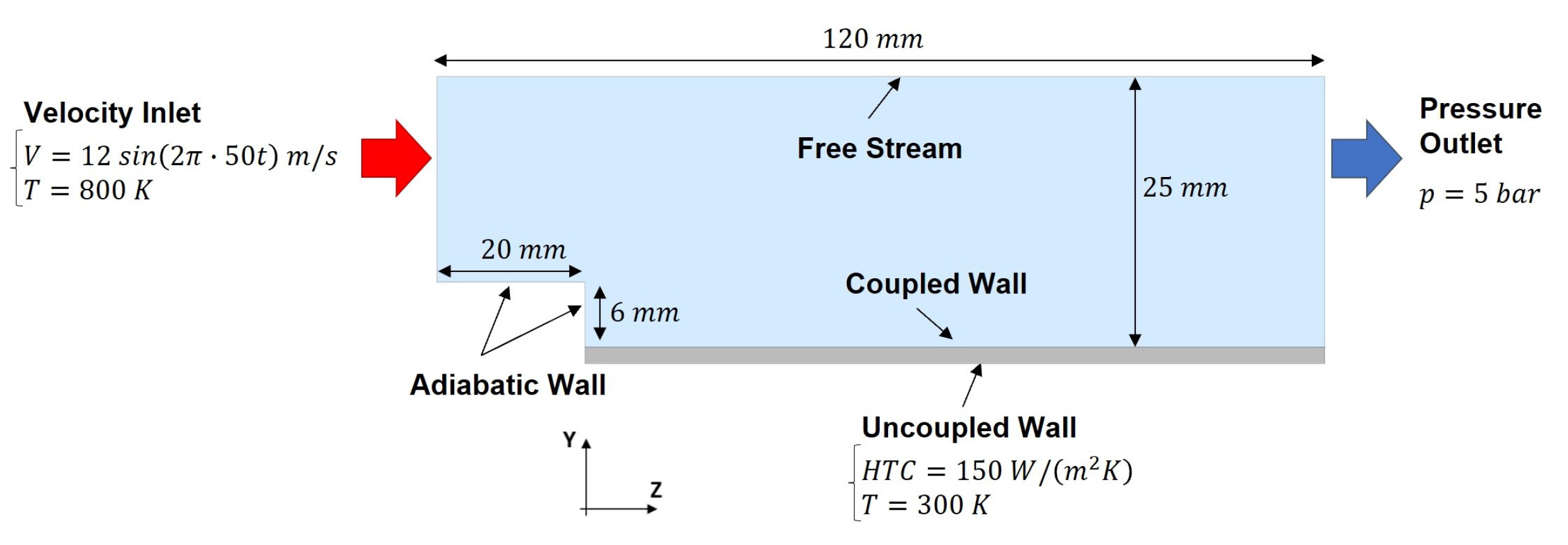
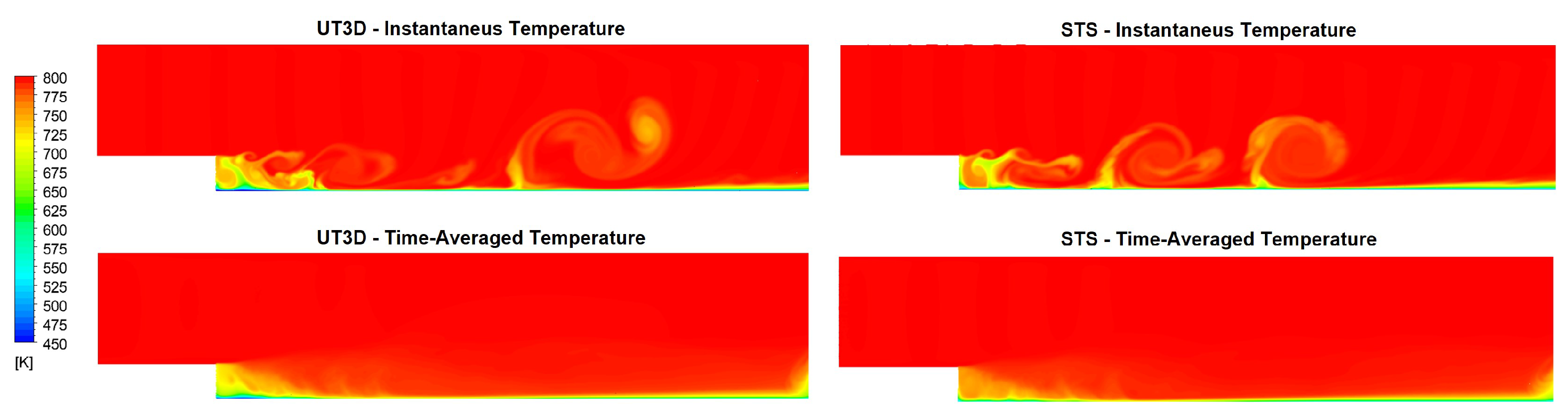
2.1. Validation of the Optimized U-THERM3D Approach

Before assessing the impact of the proposed new approach on computation time, a preliminary validation of the new tool was carried out. The test case considered was the backward-facing step that, besides being well known in the literature for many experimental [30,31], numerical [32,33,34] and heat transfer studies [35,36,37,38], was used for the first development of U-THERM3D by Bertini [23].

For the first validation, the quasi-2D computational domain, shown in Figure 3, was examined. The test case featured a channel coupled with a solid plate having a thickness of 1.5 mm. To better force the oscillatory behavior of the flow, a sinusoidal velocity condition was imposed at the inlet of the duct. The set of boundary conditions consisted of a constant inlet temperature and a convective heat flow condition on the bottom surface of the solid foil. Meanwhile, a pressure condition was imposed at the outlet section. The lateral surfaces of the computational domain were treated as symmetrical. A hexahedral grid, consisting of 800k elements, was used for the fluid domain, while 20k elements were used to discretize the solid domain. Compared with the simulations performed by Bertini [23], in which a Scale-Adaptive Simulation (SAS) approach was used for turbulence modeling, a Stress-Blended Eddy Simulation (SBES) method was used [13] in this new numerical campaign. This hybrid approach for turbulence modeling ensured an LES solution in regions where flow was not well driven, while it applied the k$\omega$-SST model [39,40] in near-wall regions, providing numerically affordable boundary layer modeling. For the CFD solver a $5\times {10}^{-5}$ s time-step was used to ensure the proper resolution of the larger turbulent length scale. Meanwhile, a $5\times {10}^{-2}$ s was used to solve the energy equation in the solid domain.

To validate the Solid Time-Step method, a numerical experiment was performed on such a test case. The two loosely-coupled approaches, U-THERM3D and Solid Time-Step, were compared with a strongly-coupled conjugate heat transfer simulation using the same mesh and numerical setup. To reduce the computational effort of the numerical test, solid domain properties were adopted to reduce the thermal inertia, and are summarized in

Table 1. Solid properties for the backward-facing step plate.

Name	Symbol	Value	Unit
Density	$\rho$	100	kg/m${}^3$
Specific Heat	$c_p$	50	kJ/kgK
Thermal Conductivity	$\lambda$	5	W/mK

. This assumption was even more legitimate since with loosely-coupled conjugate calculation procedures the temporal development that the solid components undergo is not temporally synchronized with the convective phenomena occurring in the fluid domain. Therefore, the instantaneous heat loads are not the actual ones undergone by the walls during thermal transients, and only the average heat load is the same.

The instantaneous and time-averaged temperature distributions in the CFD domain obtained by the two loosely-coupled methods are shown in Figure 4. As anticipated, the numerical approach used allowed the correct prediction of the major turbulent scales, as can be seen from the instantaneous temperature distributions downstream of the step where several vortical structures formed. The intensity of these vortices was even more emphasized by the sinusoidal velocity profile imposed. By comparing the average temperature fields, it could be seen that the two methods provided, qualitatively, the same results. Only slight differences near the edge of the step and in the middle of the recirculation zone were visible.

The time-averaged wall temperature distributions along the axial development of the plate, shown in Figure 5, also revealed no particular differences, highlighting the good agreement between the loosely-coupled methodologies analyzed. Comparing the results obtained more quantitatively, the time-averaged one-dimensional wall temperature trends for both the U-THERM3D and STS simulations are shown in Figure 6. The graph also shows the values obtained with the strongly-coupled simulation (CHT). What was highlighted above is even clearer when comparing the one-dimensional temperature profiles of the solid surface coupled with the fluid. The agreement among the three numerical methods was total and it allowed the conclusion that the STS approach enabled the achievement of the same results as the U-THERM3D simulation, while performing a single simulation and eliminating the requirement to couple two simulations solved in parallel.

It is worth underlining that the purpose of this first numerical campaign was to validate the numerical approach and to confirm that the different loosely-coupled methodologies provided the same results. The test case under investigation did not permit the evaluation of the computing savings of the STS approach with respect to the U-THERM3D one because the amount of data exchanged between the two computation domains in the U-THERM3D simulation was very small, so the execution times of the write and read phases were almost zero. The detailed analysis, in terms of computation time and savings, is analyzed below in a more challenging test case.

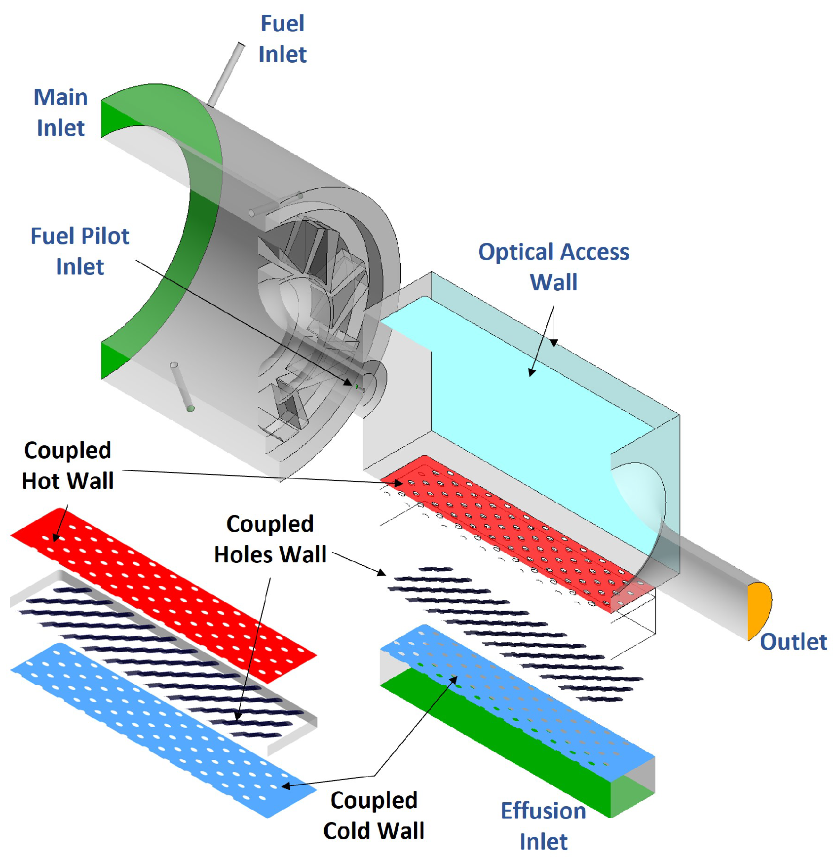
3. Experimental Test Case

The single-sector RSM combustor, which takes its name from the research institute within the University of Darmstadt, led by professor A. Dreizler, was the test case in which the advantages introduced by the newly optimized loosely-coupled methodology were analyzed. This academic burner has several interesting features that make it a very representative model of industrial combustors. It operates under pressure, and not under ambient, conditions. It can also work with both premixed and partially premixed methane-air flame conditions and, finally, it has an effusion-cooled plate. The RSM combustor is also equipped with a mobile block swirler to control the geometric swirl number, based on the TECFLAM design [41] widely studied in literature, both experimentally [42] and numerically [43].

A schematic layout of the combustor is shown in Figure 7. It has a square-section combustion chamber, bounded by three optical accesses, in addition to the aforementioned effusion-cooled plate, that allowed an extensive experimental campaign. Several operating conditions ertr tested and the related measurements of the flow field, generated inside the chamber under both reactive and non-reactive conditions, were described by Hermann et al. [25] which, for the reactive cases, also reported gas phase temperatures in different sections of interest. Wall temperature measurements and study of the structures created by the flame-cooling air interaction were carried out by Greifenstein et al. [26,27]. The reader interested in further information on the experimental tests conducted on the gas turbine combustor model, the measurements made and their uncertainties, is referred to the above-mentioned publications by Hermann and Greifenstein et al.

The main air supply system feeds the chamber, the primary air mixes with radially injected fuel and passes through the swirler. A dedicated air supply system is used for the effusion cooling system. The effusion-cooled plate is shown in Figure 8, having 145 holes with a cylindrical staggered pattern in both axial and lateral directions. The holes have a diameter of 2 mm and an inclination of 30 degrees, generating 4% porosity on the plate.

This test case was chosen because it had already been studied by the authors employing a simulation with the simplified tool U-THERM3D and was, therefore, perfectly suited for the application and verification of the STS method. In [28] a simplified version of the U-THERM3D tool was used because the impact of radiative heat transfer was neglected, due to the low emissivity level of gaseous methane–air flames. To compare the numerical results of the STS with those obtained previously in [28], the same operating point was taken into account, and the details are shown in

Table 2. Test points analyzed.

Name	Symbol	Value	Unit
Operating pressure	P	0.25	MPa
Swirl number	S	0.7	−
Oxidizer mass flow	${\dot{m}}_{ox}$	30	g/s
Oxidizer temperature	$T_{ox}$	623	K
Eff. cooling mass flow	${\dot{m}}_{eff}$	7.5	g/s
Eff. cooling temperature	$T_{eff}$	623	K
Fuel mass flow	${\dot{m}}_f$	1.128	g/s
Pilot fuel temperature	$T_{pf}$	333	K
Staging ratio	$SR$	10%	−

. The RSM combustor in reactive conditions, operating with partially premixed flame, was simulated, with a pilot fuel flow rate of 10% to the total.

4. Numerical Details

All the simulations performed in the present work were carried out with the 2021R1 version of the commercial CFD solver ANSYS Fluent [44]. As mentioned extensively above, the objective of the work was to compare the Solid Time-Step approach, versus the U-THERM3D tool, for an initial optimization step of the latter. The results provided by U-THERM3D had already been analyzed by the authors in [28]. To be as consistent as possible with the results already discussed, the numerical setup was not varied, except for changes to improve agreement with the reference experimental data. For this reason, those aspects of the computational domain, turbulence modeling, and combustion model that did not change from the numerical reference work are only discussed briefly in the following paragraphs. In this paper, only the basic information is provided to get a complete overview of the numerical approach used, but the interested reader can find all the details in [28]. The following paragraphs highlight in detail the changes made from the baseline U-THERM3D simulation.

4.1. Turbulence Modeling

The numerical campaign was carried out with two different turbulence models. As performed in [28], for the first simulation the hybrid RANS/LES model named Stress-Blendend Eddy Simulation (SBES) [13] was used. With this approach, k$\omega$-SST model [39,40] was employed to solve near-wall regions, whereas the flow field was solved in an LES manner in the freestream. The transition between RANS and LES behaviors was handled internally by a blending function [44] that defined the SBES sub-grid stress tensor. For the modeling of the sub-grid stresses in the LES part, the Dynamic–Smagorinsky model was adopted [45].

After this first calculation, a full-LES simulation was carried out with the same sub-grid model to assess the impact of the latter on wall heat fluxes. The purpose of the present work was to apply, for the first time, the Solid Time-Step procedure for the prediction of thermal loads on solid surfaces, optimizing the workflow of the U-THERM3D procedure. For this reason, it was decided to proceed as linearly as possible, carrying out a first simulation with the STS method and the same SBES model used in the reference U-THERM3D simulation, and, thus, reducing the sources of uncertainty. After that, the full-LES calculation was computed.

4.2. Combustion Modeling

For the treatment of combustion, the same strategy was used as in [28], based on the Flamelet Generated Manifold (FGM) model [46]. This flamelet-based approach is widely used for combustor CFD gas turbine simulations [24,47], in which a lookup table is created from the resolution of 1D laminar flamelets. In this framework, the reactive flow behaviors depend only on two quantities, i.e., the mixture fraction Z and the progress variable c, which is a dimensionless index of how far the chemical combustion reaction has advanced toward the products, defined as the ratio of the mass fractions of CO and CO${}_2$ to their values at local equilibrium [48]. The model is also based on the transport of two additional equations for the variances of mixture fraction and progress variable [49], while, to take into account the effects of turbulence, the finite rate closure is used. Regarding the fuel composition, the same natural gas mixture as in the experimental test was employed, specified in [26], for which the GRImech3.0 [50] kinetic mechanism, based on 325 reactions and 53 species, was used.

Temperature-dependent properties were defined for the reactive mixture through the open-source suite for chemical kinetics Cantera [51].

4.3. Computational Domain and Boundary Condition

The considered computational domain was consistent with the experimental apparatus and is reported on in Figure 9. The domain had a mixing zone for primary air and fuel, which was injected radially with respect to the axis of the burner. After passing through the swirler, the mixture was free to react within the flame tube and the burned gases then flowed toward the outlet of the computational domain through a convergent section. The entire cooling system was simulated explicitly, so every effusion hole was present within the domain, including a portion of the refrigerant supply plenum. The only solid part in the simulation was that related to the effusion-cooled plate, which was an alloy metal modeled with temperature-dependent properties. In this work, contrary to what was done in [28], the solid plate was directly included in the computational domain. The STS method allowed a specific time-step to be set for both the solid parts and the gas phase, eliminating the problem of having to perform multiple simulations in parallel that exchange information with each other to update the coupled thermal boundary conditions.

The same mass flow rate value relative to the reference experimental test [25,26] shown in Table 2 was imposed for all the above-mentioned inlets. Meanwhile, the operating pressure was imposed at the outlet.

The main difference from the experimental rig concerned the pilot fuel duct. During the numerical campaign, conducted in [28], the pilot fuel duct was reduced to ensure that the pilot jet entering the chamber was solved in an LES manner. A fully developed velocity profile, [52] with a synthetic turbulence generator [44], was imposed with a 12.73 m/s mean value to match the experimental fuel mass flow rate. Since an overestimation of the pilot jet penetration, ascribable to the use of integral values for the turbulent boundary conditions imposed on the inlet, was observed in the previous numerical campaign, in this new numerical task, profiles were also imposed for the turbulent quantities to improve the agreement with the experimental data.

In [28] it was extensively discussed that the behavior of the pilot fuel jet strongly impacted the whole combustion chamber. The opportunity to be able to change boundary conditions to improve agreement with the experimental data directly in the STS simulation was made possible by the complete validation of the model described in Section 2.1.

Concerning other numerical aspects, the same assumptions made in [28] were also adopted in this paper. In particular, the identical temperature and composition-dependent properties were used for the gas phase by means of the same UDF used in [28]. As already mentioned, the impact of radiative heat flux was neglected given the low brightness of the methane flames. The same treatment was also adopted for the quartz surfaces, meaning they were imposed at a fixed temperature of 1300K, based on the preliminary RANS campaign conducted in the test case; the results of which are reported in the above work.

4.4. Computational Grid and Numerical Setup

As already mentioned, the STS method allowed simulation in a single ANSYS Fluent session of both the gas phase and the solid parts with a different time-step. Compared to the previous activity [28], a new mesh was generated that also included the solid plate. The creation of the computational grid was done using ANSYS Meshing by imposing a general sizing of 1 mm and 5 prismatic layers at the walls, Figure 10. To be consistent with the mesh used for the reference simulation, the same sizing and refinement were adopted. To capture the overall development of turbulent structures, the swirler and primary zone regions were discretized with 0.45 mm elements. Additional thickening with 0.1 mm elements was adopted for the pilot fuel jet injection region. A dimension of 0.15 mm was used to discretize the effusion holes, while 0.75 mm elements were used for the near-wall region of the plate, to correctly predict the effects of inlet and trails exiting the effusion holes. The mesh obtained had globally 66 million polyhedral elements, of which 42M were related to the fluid domain, the same size that was also obtained in [28]. The 24M remaining elements belonged to the solid domain. Compared to the mesh generated for the U-THERM3D simulation of the solid domain used in [28], 7M of the new mesh was much finee, but should not be surprising, as this was affected by the refinements performed on the fluid domain in the near-wall regions. In any case, as is discussed in the following sections, this increase in grid elements had no impact from a computational cost point of view.

The generated mesh was used for both SBES and LES approach simulations, as it satisfied Pope’s criterion [53], thus, allowing the resolution of the 80% of the turbulent large scale that ensured good quality in the LES solution [8,24,28,54].

Coherently with what was done in [28], in this new numerical activity the SIMPLEC pressure-based algorithm was also employed with a second order upwind scheme for all equations, except for time discretization, for which the second order implicit formulation was applied. The time-steps used for the two parts of the computational domain were kept unchanged from the U-THERM3D simulation [28]. In fact, $1\times {10}^{-6}$ s was used for the gas phase, while $1\times {10}^{-3}$ was used for the solid part. With the time-step fixed, the simulations were performed by executing two fluid domain flow-through times for the flushing of the quantities and, then, two flow-through times to average them, so as to ensure the convergence of the first statistical moment. Consequently, the solid domain was simulated for a total time of 60 s.

5. Results

In this section, the numerical results obtained with the STS, using both SBES and LES models, was compared with those obtained through the simplified U-THERM3D procedure, analyzed in [28], and the reference experimental data. The results firstly focused on the analysis of the flow and temperature fields within the combustion chamber and, then, focused on the wall temperature maps. After verification of the results, the calculation times of the different simulations were analyzed, highlighting the critical issues of the U-THERM3D procedure and the savings obtained with the STS method. For complete contextualization of the data, a brief description of the super-computing center used is also provided.

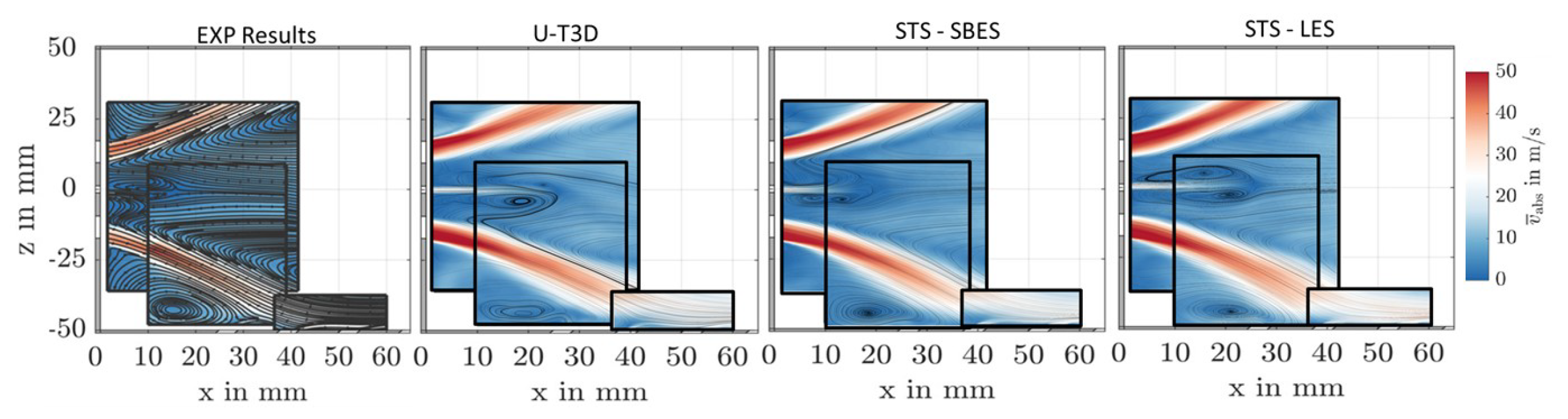
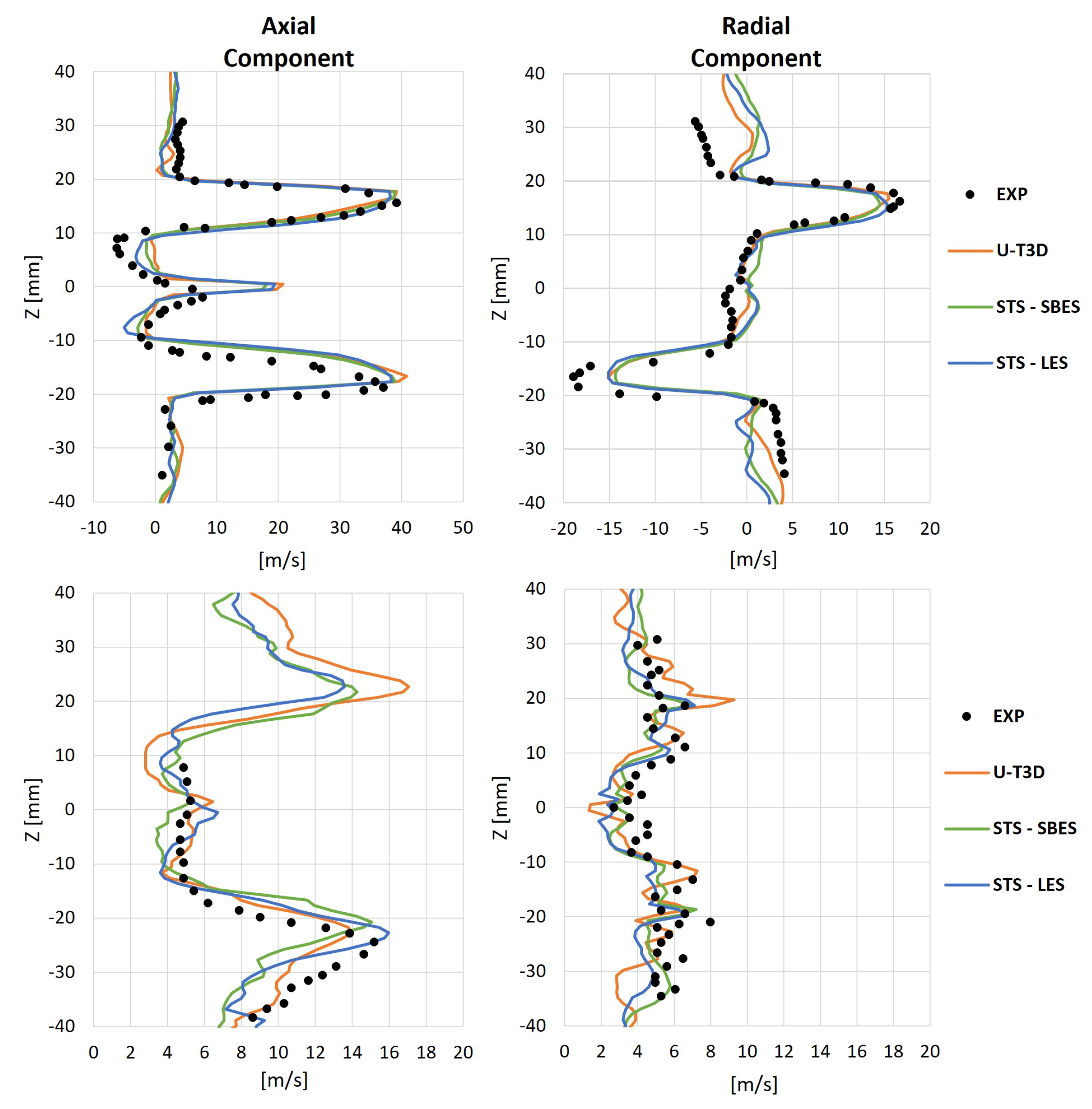
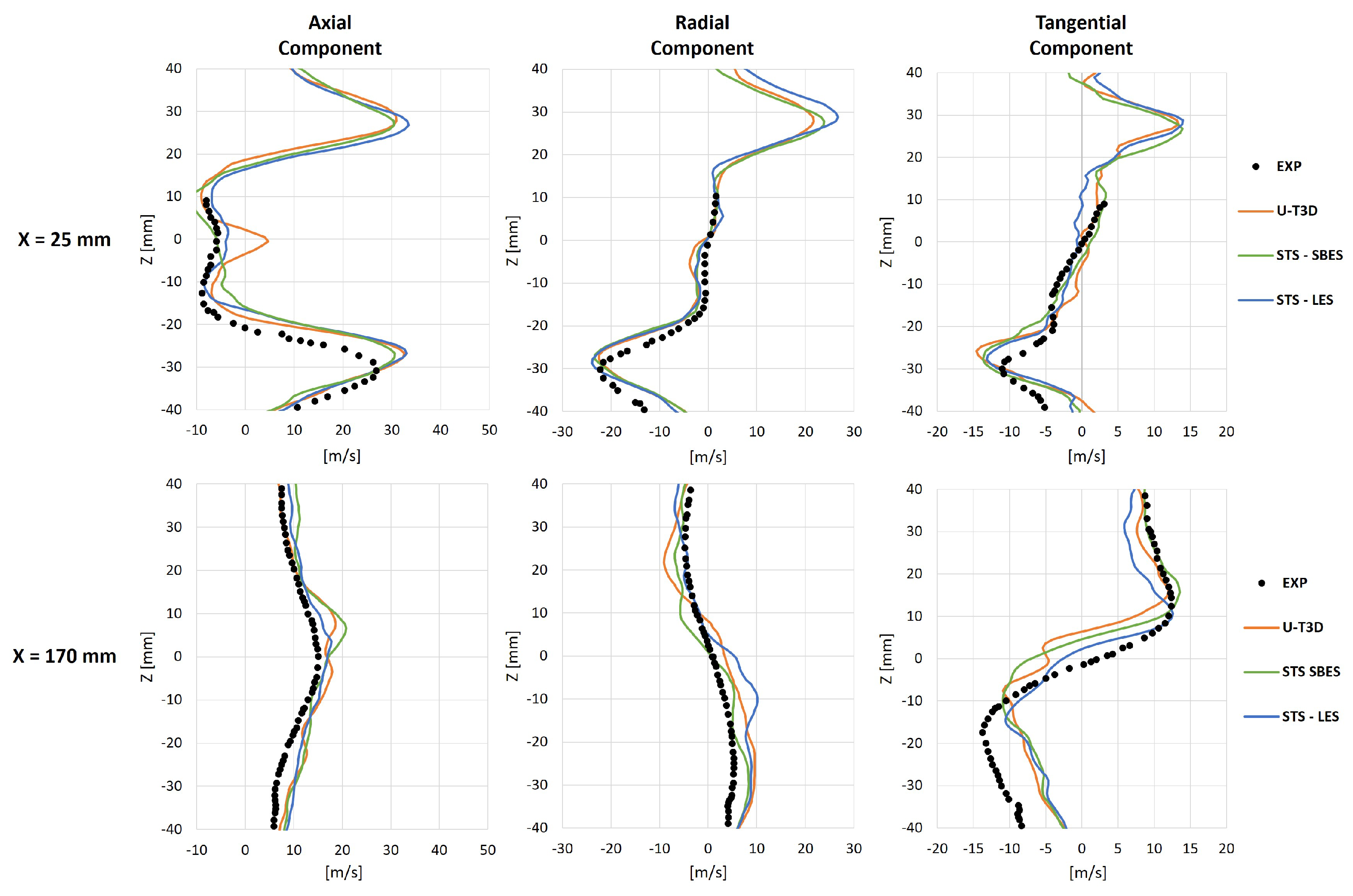
5.1. Gas Phase Velocity Fields

From the comparison of the velocity fields in the primary zone of the combustion chamber in which the swirl flow was present, shown in Figure 11, it was noticeable how all simulations provided an accurate prediction of the swirling flow structures. The vortex in the Outer Recirculation Zone (ORZ) of the swirled flow was well predicted by both simulations with STS and was very similar to that measured experimentally in [25]. The less contracted shape of ORZ vortices, predicted by STS simulations compared with the U-THERM3D simulation, could be due to the less invasive handling of the thermal boundary conditions between the gas phase and plate wall. It is worth mentioning that at each update of the U-THERM3D simulation, new wall temperature values were set for the coupled surfaces of the CFD domain, while new convective heat flux was fixed on the solid surface of the effusion-cooled plate, operations, which inevitably led to discontinuities of the local thermal fields in the near-wall regions. Although the two simulations with STS were very similar in proximity to the effusion-cooled plate, it was possible to see a more intense recirculation for the LES simulation, in which higher velocities were reached, implying more interaction between the swirled flow and the effusion-cooled wall.

Well-developed vorticity structures could also be observed for the Inner Recirculation Zone (IRZ), but they appeared to be shifted forward with respect to experimental PIVs. Despite the imposition of turbulent profiles at the pilot jet inlet, simulations with STS predicted jet behavior would still be penetrating. For the LES simulation, it can be noted that the vortices triggered by the shear layer of the pilot fuel jet were closer to the bluff body than for the two SBES approaches, an indication of more intense mixing.

From the radial profiles of the velocity components, it was possible to confirm the above considerations. In Figure 12 the velocity profile of the axial and radial velocity components are shown, together with the Root Mean Square (RMS) values at a distance of 5mm from the bluff body and equivalent to two diameters of the pilot fuel supply duct. From this detailed comparison, it was possible to observe that there was an overestimation regarding the pilot fuel jet penetration, since the velocity predicted by the simulations was about twice the experimental one. Concerning the swirl jets these were well reconstructed in terms of both axial and radial velocity, with only a slight displacement of the swirl jet interacting with the effusion-cooled plate being seen, identified by the negative Z coordinate. That obtained by the simulations was a swirl flow, that was almost symmetrical with respect to the axis of the combustor chamber. Whereas from the experimental evidence, the latter seemed more open toward the plate. This was confirmed by the fact that the minimum radial velocity value was not equal in absolute value to the maximum. Since only the part of the swirl jet interacting with the coolant air was not correctly predicted this could be due to a different behavior of the first rows of effusion holes between numerical and experimental results. Moving to the radial RMS distributions of the two velocity components it can be seen that the proposed numerical approaches could correctly capture turbulent fluctuations. In fact, both in terms of shape and numerical values, the predicted numerical profiles were very close to the experimental ones.

Moving far from the bluff body, the agreement between simulations and experimental data improved. Figure 13 shows the velocity profiles of all three components at 25 mm and 170 mm of the burner axial coordinate. What can be immediately noticed in the first section is that the axial velocity profiles of the STS simulations were no longer affected by the presence of the pilot fuel jet, as in the U-THERM3D simulation, due to the change in the turbulent boundary condition imposed on the fuel pilot inlet, which promoted faster mixing within the combustion chamber. It was also possible to see a slight difference in terms of the shape of the lower swirl jet predicted by the simulations, resulting in a modestly more closed flow, compared with the experimental data. In addition, the velocity profiles in this section confirmed that the LES simulation had a slightly faster swirled flow than the SBES calculation, so more interaction between the swirl flow and the coolant air could be expected. Analyzing the profiles before the beginning of the converging section at the combustion chamber outlet, it can be seen that the agreement was almost total for the axial and radial velocity components, while there was an underestimation of the tangential component in the lower part of the combustion chamber for all reported numerical approaches. This trend could be due to excessive coolant accumulation in the near-plate regions, which tended to dampen the tangential swirl flow wakes against a slight overestimation of the other two velocity components, which might be more affected by jets exiting the effusion holes. Unfortunately, no visualizations of the flow field in the zones near the plate were available for this axial quota, and, at the same time, all experimental data stopped at 10 mm from the effusion-cooled plate, so it was not possible to better contextualize the numerical results.

Moving the analysis to the radial distributions of the RMSs of the three velocity components, shown in Figure 14, it can be seen that in the central region downstream of the pilot jet, i.e., 25 mm from the burner, the agreement improved by passing from the SBES approach to the LES approach. This trend confirmed what had been analyzed previously, namely that the application of turbulent profiles to the pilot jet inlet not only promoted mixing, but also moved the numerical results closer to the experimental ones. This confirmed the authors’ conclusions in [28], in which it was stated that the excessive penetration of the pilot jet could be partly due to underestimation of turbulent structures. Focusing attention on the portions closest to the perforated plate, i.e., in the RMS profile of the axial velocity component at 25 mm, confirmed what has already been said for the velocity profiles; a more closed swirl flow predicted by numerical simulations led to an underestimation of vortex structures. For the other two components, instead, total agreement with the experimental data was noted.

For the sections near the combustion chamber outlet there was an underestimation, in terms of RMS, of the axial component, but of rather limited magnitude. For the other two components, the same conclusions could be drawn as for the velocity profiles, namely, that the underestimation near the effusion-cooled plate could be due to an overly cohesive layer of coolant.

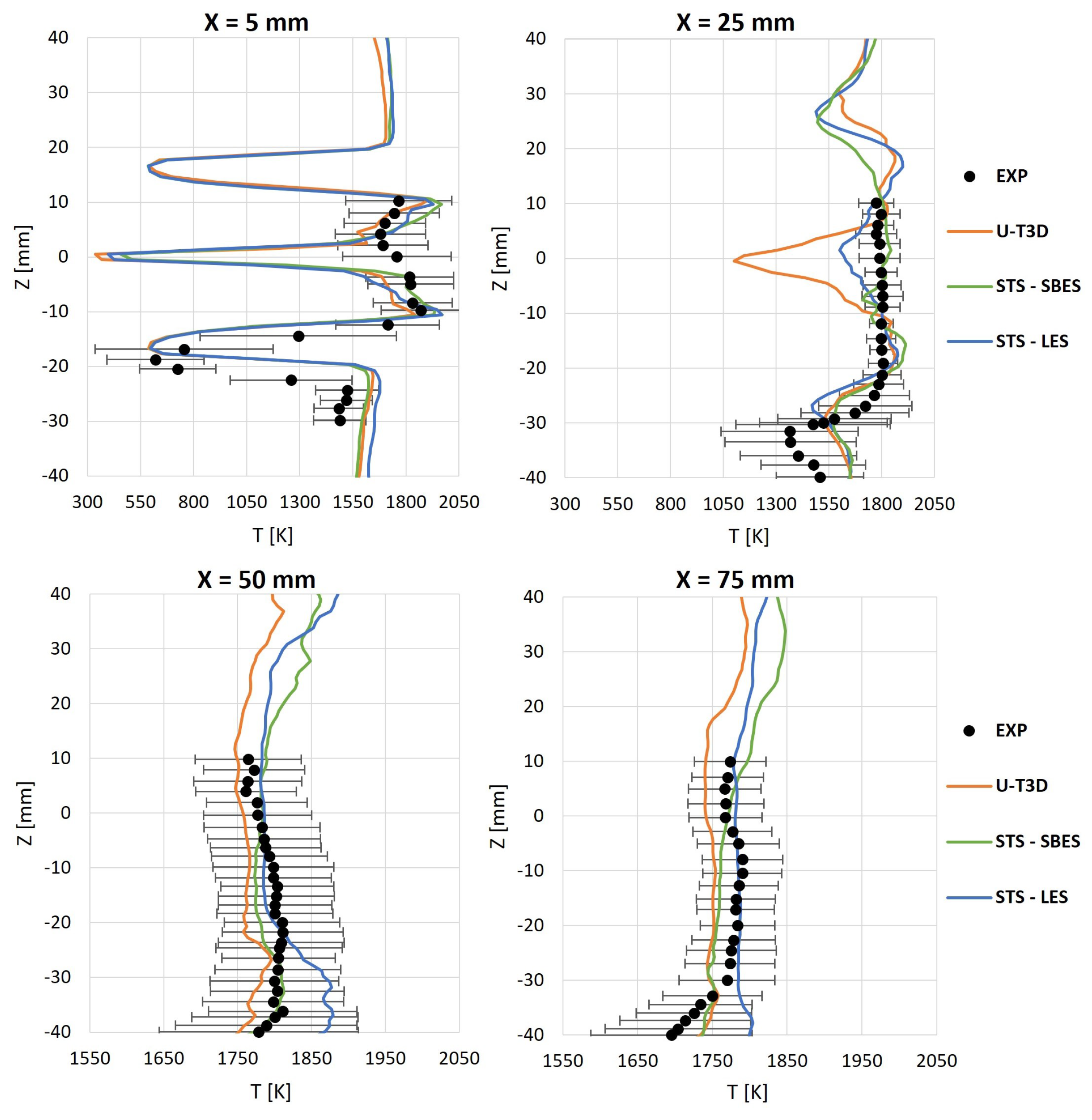
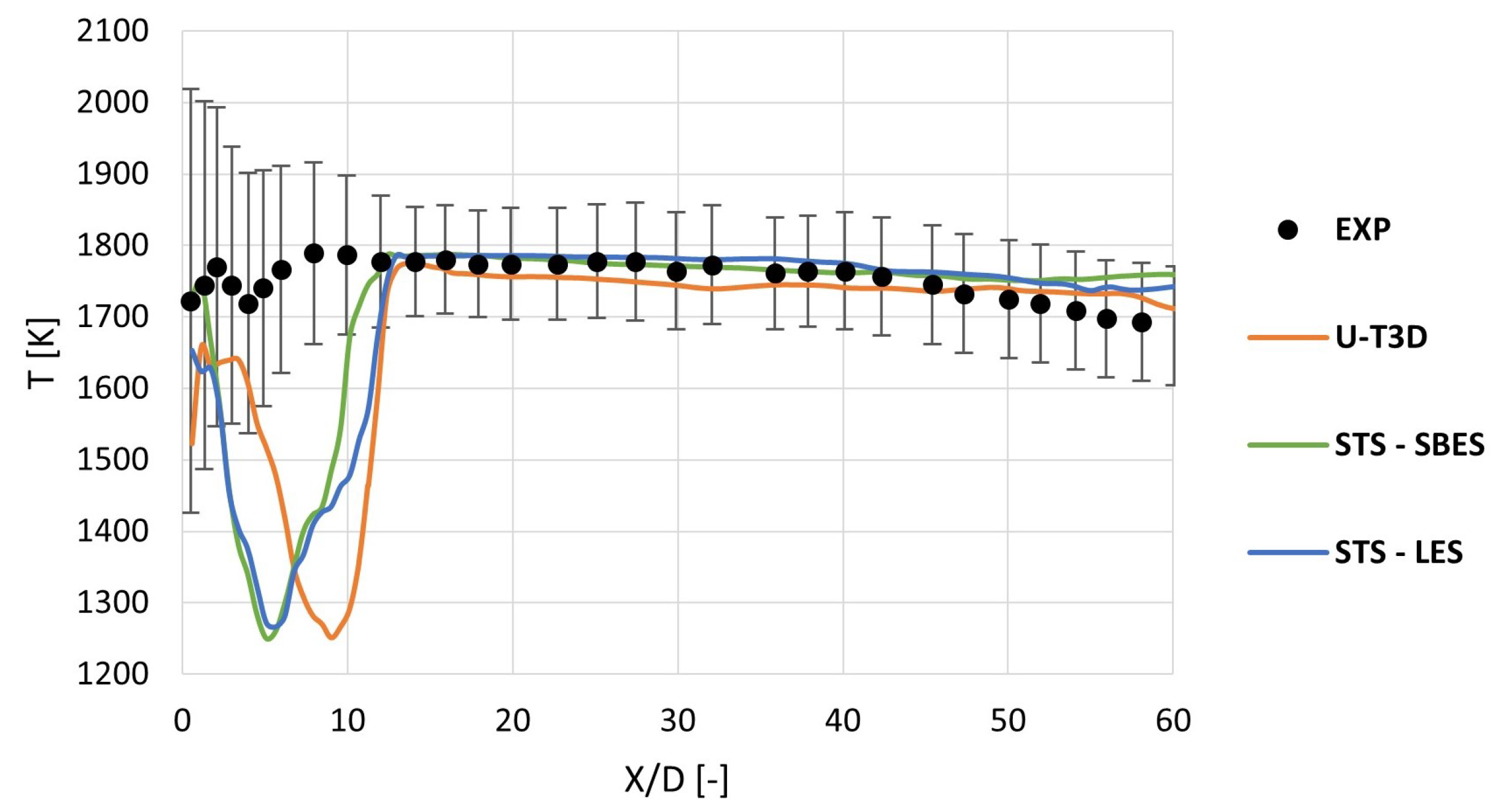
5.2. Gas Phase Temperature Fields

The time-averaged temperature maps, obtained by the STS method and by the U-THERM3D simulation from [28], are shown in Figure 15. It can be seen that the three simulations were in agreement with each other, but by focusing on the IRZ, the impact behavior of the pilot fuel jet has on the entire combustion chamber was, once again, evident. The temperatures in the flame tube were higher in the simulations conducted with the STS than in the U-THERM3D simulation. From these, it could be observed that the pilot jet of fuel, although it had a penetrating behavior, had a greater diffusion within the primary region increasing the reactive process rate. Comparing the two STS simulations, it could be observed that a more intense reaction occurred near the shear layers of the swirled flow in the LES calculation favored by the increased mixing near the bluff body already described by the analysis in Figure 11.

To better quantify the differences between the three simulations analyzed, the radial temperature profiles in four relevant sections are shown in Figure 16. The graphs also present the minimum and maximum temperature bars acquired during the experimental test. From the 5 mm profiles, the temperature underestimation in the central region of the combustion chamber, in which the pilot fuel jet was present, is evident. In fact, in this section, experimentally, the presence of unburned fuel was no longer detected, while, numerically, there was a temperature value close to its injection value of 333 K. From this profile, the slight shift in the prediction of the swirled jet discussed earlier in the velocity profiles analysis could be observed again. The section at 25 mm from the bluff body was particularly interesting, to better understand how far the pilot jet was penetrating within the combustion chamber. While for the U-THERM3D simulation, the unburned jet was evident in the central area, the STS simulations showed, instead, a reacted flow, in which only a small part related to the pilot jet remained visible for the LES simulation. Moving closer toward the cooled plate, the gap between experimental and numerical results increased, probably due to less interaction between swirl flow, which was slightly more closed, and cooling air leading to less turbulent mixing. Moving downstream the radial temperature profiles tended to have an excellent agreement in the central areas of the combustion chamber. Even if the LES simulation showed an overestimation of temperature in the region closer to the plate, compared with the experimental values, it was still within the range of measured data.

The goodness of temperature prediction in the central part of the combustor is well evidenced in Figure 17. To better understand the results, these were plotted along the axial abscissa scaled with respect to the diameter of the pilot fuel jet. The profiles shown were obtained by averaging over a circular sector with a diameter of 2.5 mm, the same as for the duct fuel pilot. Based on what was discussed in [28], this approach was preferred because, experimentally, an extremely high value was measured near the bluff body, which was typical of an already reacted mixture, even where pilot fuel injection occurred. This behavior was particularly strange, unless, experimentally, the mixture reacted directly within the duct or there was some pulsating effect that might have affected the measurement. Within the first ten through diameters, the simulations severely underestimated the temperature, because in this zone the mixing of the fuel that was taking place would only later bring it to the condition when it would be able to react. Please note that the pilot fuel injection temperature was set to 333 K, according to the data given in [25,26], but it must be specified that possible heating effects of the pilot fuel in crossing the duct was neglected in the simulations, due to lack of further data to estimate it. In any case, it was considered improbable that this effect would lead to the full match of the experimental data in the zones closest to the bluff body. After this region, the numerically-obtained profiles coincided with the experimental values, so the reactive conditions inside the combustion chamber were well predicted by all numerical approaches.

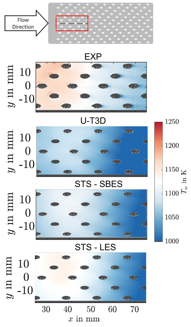
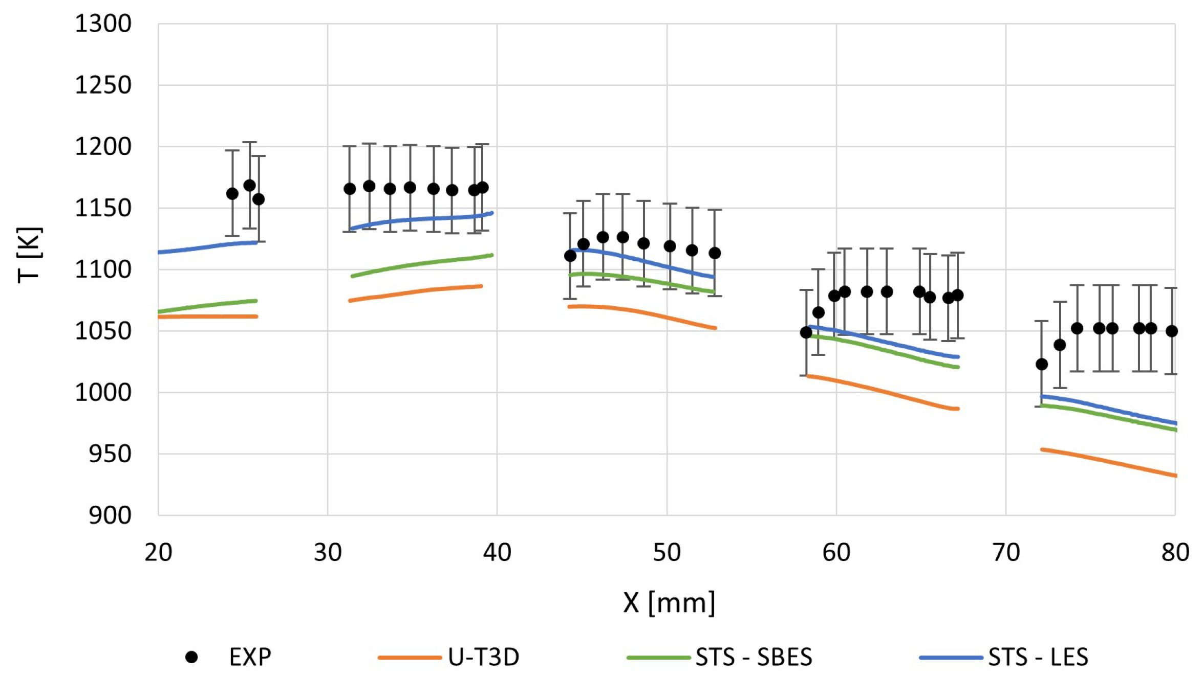
5.3. Effusion-Cooled Plate Wall Temperature

Figure 18 shows the temperature maps obtained through different multiphysics and multiscale approaches used and are limited, experimentally, to the highlighted portion of the effusion-cooled plate investigated by Greifenstein et al. [26]. Although there was a gradual improvement in agreement with the experimental data, the wall temperature maps obtained by the STS method continued to underestimate the experimental value obtained in [26]. The U-THERM3D simulation that was carried out in [28] was performed with the same computational grid and with the same SBES numerical approach, so it became evident how the behavior of the pilot fuel jet also impacted the wall heat transfer, and how critical its modeling was, since it strongly influenced the reaction in the primary region. Specifically between the two central maps in Figure 18, only the boundary condition related to the turbulence imposed on the pilot fuel jet inlet changed and the latter was derived from the previous simulation U-THERM3D. As was also observed in detail from the analysis of Figure 15, the different modeling of the jet led to a non-negligible change of the entire temperature pattern within the combustion chamber. Although the change brought the numerical result closer to the experimental data, this was still not sufficient for the correct prediction of heat fluxes reaching the effusion-cooled plate. In particular, by focusing on the temperature map obtained by the LES approach, part of the gap with the experimental result further reduced. This result allowed the conclusion that part of the underestimation was due to the modeling of sub-grid turbulence. The SBES simulations adopted a k$\omega$-SST RANS turbulence model for the near-wall region, which did not seem to be the most suitable for predicting the proper behavior of an effusion cooling system. This RANS model led to an excessive underestimation of vortex structures that should be generated near the wall by all the effusion jets entering the chamber and, consequently, limited the turbulent mixing between the combustion gases and the coolant air. Thus, it generated too thick a layer of coolant air on the wall and, finally, held the plate at a lower temperature than it should have been at.

As can be seen from the one-dimensional wall temperature profiles in Figure 19, the difference between the numerical results and the experimental measurements greatly reduced for the STS–LES simulation. The data in the graph was discontinuities where the plate symmetry plane cut the effusion cooling holes. The beginning of the measurement portion of the effusion-cooled plate was located near the outer recirculation zone (ORZ). From what is seen in Figure 11, the vortex reproduced by the LES simulation was the one closest to the experimental. The higher vortex intensity brought greater recirculation of burned gas and, consequently, an increase in local temperature. The temperature peak reached near 40 mm was well predicted by the LES simulation, which presented the greatest swirling flow-cooling air interaction, that led to a significant impingement on the cooled wall. In this portion of the plate, the results differed from experimental results by 15 K. On the contrary, the SBES simulations presented the same temperature level at the beginning of the plate, which was lower with respect to the one computed by the STS–LES calcualtion. However, the simulation with STS had a more pronounced thermal gradient, due to the higher reactivity in the primary zone generated by the faster mixing of the fuel pilot jet. As seen from Figure 15, the STS simulations had higher temperature zones near the walls propagating from the high reactivity region of the IRZ. This once again confirmed how complex the flow and thermal fields of this academic combustor were, and how the pilot fuel jet modeling was a key aspect in correctly predicting not only the velocity and temperature of the gas phase inside the combustion chamber, but also the thermal flux reaching the walls.

The same conclusions could also be visualized in terms of total cooling effectiveness ${\eta }_{TOT}$, defined as in [26], and according to Equation (1). $T_{\infty }$ represents the temperature of the burned gas that not affected by the cooling system. This term is defined as the temperature along the combustor centerline in the post-flame zone. Given the good agreement of the simulations with the experimental data in the considered combustor zone, shown in Figure 17, it was decided to take the same value used in [26] and equal to $T_{\infty }=1775$ K. The other two terms appearing in the equation are the wall temperature, obtained by the multiphysics and multiscale simulations, denoted with $T_w$, and the cooling inlet temperature, $T_c$, set constant and equal to what is shown in Table 2, as in the experimental work [26]. Due to the definition used for total cooling effectiveness, the trend obtained was nothing more than a scaled function of the wall temperature and, therefore, the agreement between the numerical and experimental data was the same as that shown in Figure 19.

$${\eta }_{TOT}=\frac{T_{\infty }-T_w}{T_{\infty }-T_c}$$

(1)

In CFD simulations conducted with the STS method, a passive scalar was injected at the cooling system inlet. It gave an indication of how the coolant was distributed over the effusion-cooled surface. Furthermore, this quantity could be interpreted as an adiabatic cooling effectiveness, ${\eta }_{AD}$, in analogy to Pressure Sensitive Paint (PSP) experimental techniques conducted under truly adiabatic conditions [55,56,57].

Figure 20 shows the adiabatic effectiveness maps obtained by the CFD simulations. Both have the respective total cooling effectiveness isolines superimposed, as defined in Equation (1). The minimum value of this quantity was set to, and limited to, the lowest measured value, visible in Figure 21, to simplify visualization of the isolines. From the maps, it is possible to visualize the distribution of the effusion coolant flow over the plate. In the central portion at the beginning of the plate, the typical effect of swirling flow on an effusion-cooled plate, identified by the low-efficiency zone, can be seen. Minimum coverage was achieved where the interaction of the swirling flow with the plate occurs led to the inevitable washout effect that destroyed all the coverage provided by the coolant.

These maps allow further justification for what has already been discussed for the velocity maps in Figure 11, as well as the one-dimensional wall temperature profiles in Figure 19. In the initial portion of the cooled plate, near the first row of effusion holes, it could be noted that the adiabatic effectiveness was lower for the simulation performed with the LES approach. This was due to the greater intensity of the vortex structure present in the ORZ, which promoted mixing and tended to bring more hot gas flows near the plate. While no particular differences were evident in the central portions of the cooled plate, the situation changed at the end of the plate where there was a high accumulation of coolant, even more present in the LES simulation. Again, the results were in agreement with what had already been stated in the discussion of velocity profiles at 170 mm (Figure 13), regarding the near-wall region flow.

Exploiting all the results shown so far, it could be concluded that the simulation with the hybrid SBES approach suffered in predicting the turbulent magnitudes in the proximity of the effusion-cooled wall, due to the underestimation of the turbulent structures that should be created in the wakes of the effusion holes and, thus, in the interaction between the coolant flow and the hot gases. On the other hand, the simulation with the LES approach seemed to partially mitigate this phenomenon by ensuring proper mixing between the hot gases and the coolant flow outside the shear layer and, thus, predicting a heat flow on the cooled wall that was more in agreement with the experimental evidence.

By comparing axial and radial velocity maps near the second and third central rows of effusion holes in Figure 22, it was possible to have further verification of what was previously stated. In fact, it could be observed that the swirled flow tended to interact more with the effusion-cooled plate in simulations with STS, especially for the LES approach, pointing out once again how the near-wall region RANS modeling had no negligible impact on the prediction of turbulent structures. Regarding this, it was possible to see how the velocity distributions of the two SBES approaches were similar to each other. The same trend could also be observed from the radial velocity distributions, in which less penetrating effusion jets could be observed for simulations carried out with the STS–LES approach.

Despite the agreement with the experimental data increasing in the STS–LES calculation, it was quite clear how all numerical approaches underestimated the blocking effect of the swirled flow on the first rows of effusion holes. The maps highlighted even better what emerged from the analysis of the velocity profiles regarding the position of the swirled jet, in Figure 13, and better contextualized the underestimation of the plate wall temperature in its initial zone, in Figure 19. Another important aspect to be careful about when analyzing the radial velocity maps was that Greifenstein et al. in [26] showed two operating configurations for the cooling system during experimental tests. The author referred to two working conditions: the first, in which there was an effective coverage contribution made by the holes where the radial velocity was positive, shown effectively in Figure 22, and a second, in which the holes were instead affected by a negative radial velocity that minimized the entry of coolant into the combustion chamber. For the chosen test point, the experimental behavior shown in Figure 22 was recorded on 66% of the measured samples. Such detailed evaluation was not conducted numerically, but, in light of the results obtained, a greater investigation of the behavior of the effusion cooling system is necessary to better understand the discrepancies between simulations and experimental results. In fact, a more stable behavior of the cooling system, in terms of the flow rate released from the numerically predicted effusion holes, could lead to a higher coolant presence and, thus, an excessive lowering of wall temperatures.

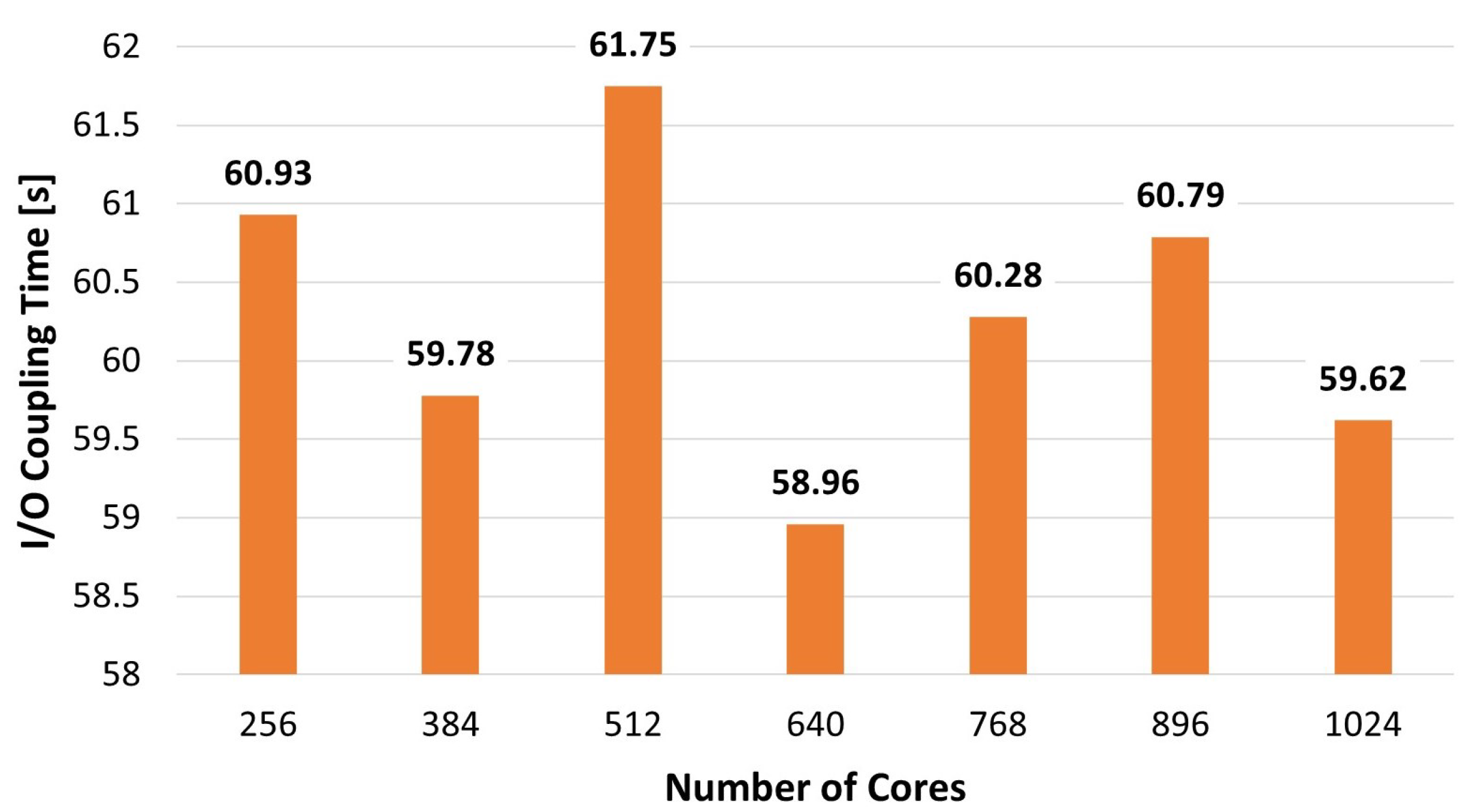
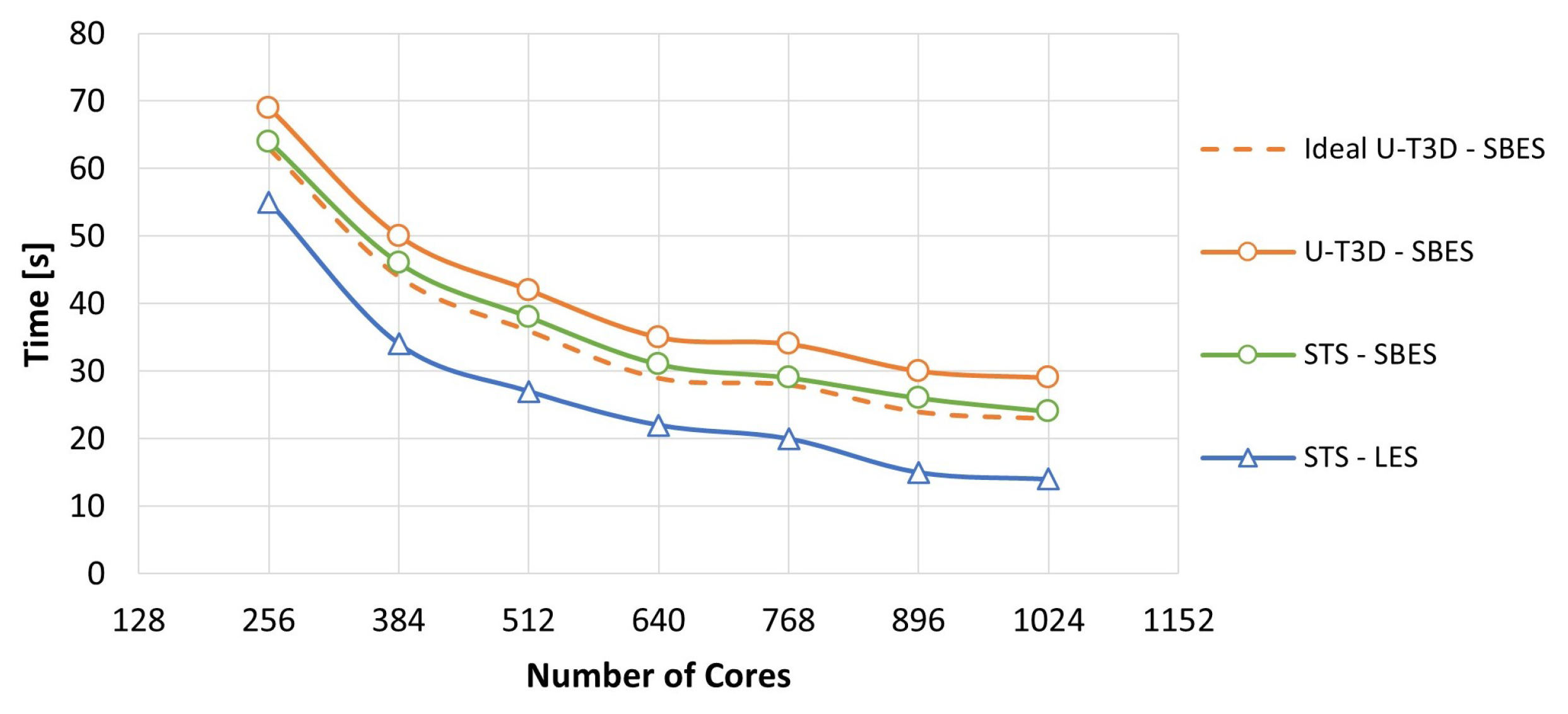
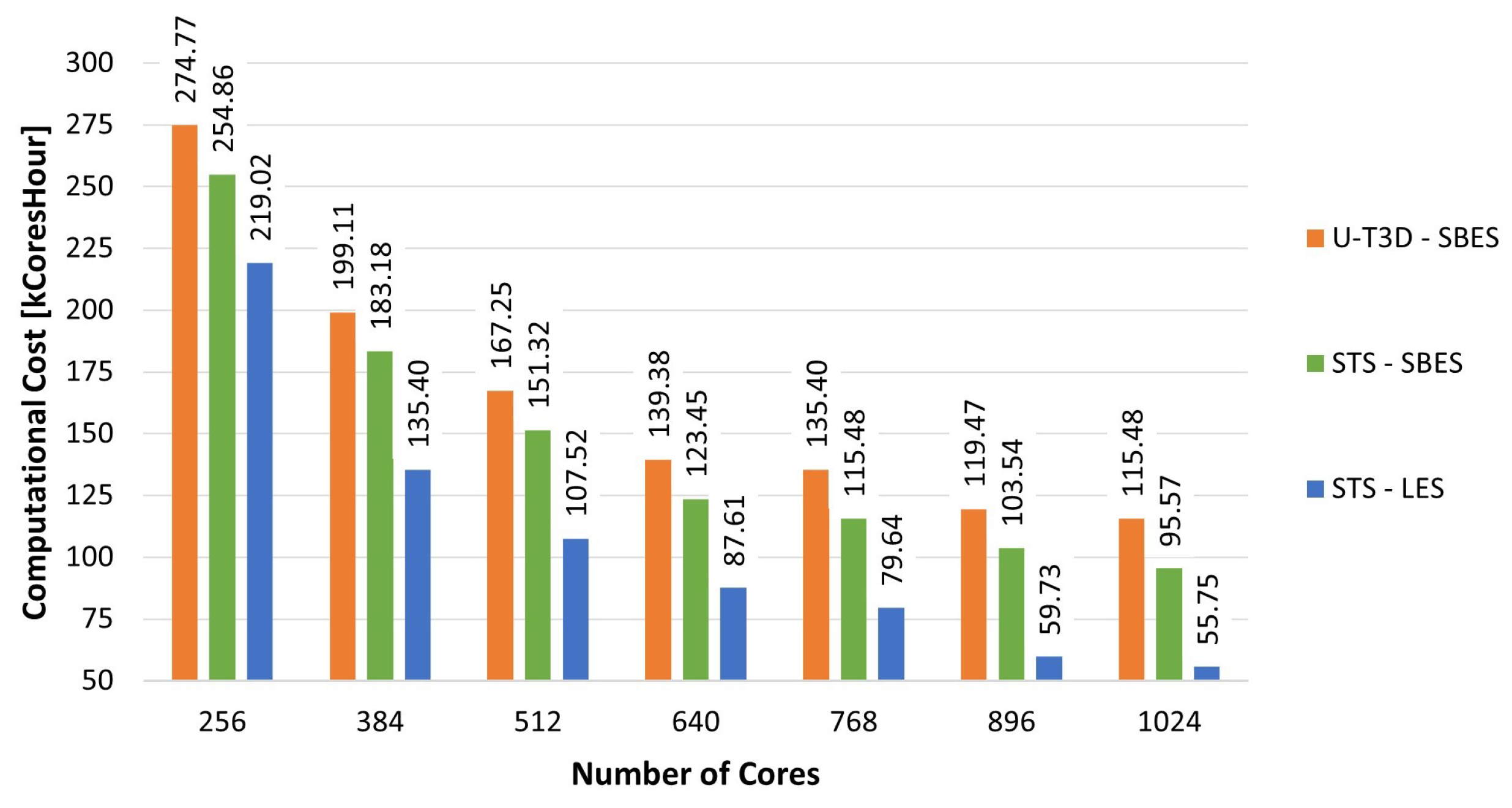
5.4. Computational Cost Analysis

Before entering into the discussion regarding computation times, it seems proper to give a brief description of the super-computing center used to carry out the entire numerical campaign presented. The computing infrastructure used was the cluster named Karolina, owned by IT4Innovations National Supercomputing Center, in the Technical University of Ostrava of the Czech Republic. The petascale system employed consisted of 831 computing nodes, of which 720 were CPUs. Since CFD simulations with the ANSYS Fluent solver were conducted exclusively on CPUs their main characteristics are summarized in

Table 3. Characteristics of the CPU compute nodes of the IT4I Karolina cluster.

Parameters	Specifications
Processors	2× AMD ZEN 2 EPYC 7H12 2.6 GHz
Number of Cores per Compute Node	128
RAM per Compute Node	256 GB
Max Memory Bandwidth	190.7 GiB/s
Interconnection	Infiniband HDR 200 Gb/s

.

Figure 23 shows the scalability performance of the CFD solver tested with the numerical RSM combustor reactive test case running on the Karolina cluster, calcolated as in [58]. Due to the high number of computational grid elements, performance could not be tested on a single node of the cluster, due a minimum memory requirements. As can be noted from the graphs, the ANSYS Fluent solver performed very well up to eight computational nodes, a range in which it had an almost ideal efficiency and a linear speedup.

The RSM combustor simulations were performed by fixing the number of time-steps to be simulated, ensuring a minimum physical time of two flow-through times for the fluid domain. To obtain a statistically independent first moment, two additional flow-through times were performed to average all quantities of interest, for a total of four flow-through times. To perform a detailed comparison of the calculation times of each proposed numerical method, it was, therefore, convenient to refer to the time required to perform a single fluid time-step.

Regarding the simulations carried out with the STS method, there was no difficulty in monitoring the calculation time of a single time-step, and neither was there for the U-THERM3D simulation, but it is worth mentioning that the latter was composed of several simulations carried out in parallel, that exchange data with each other, to update the coupled boundary conditions every ten fluid time-steps. Therefore, part of the work focused on quantifying the time required for input/output operations between the two coupled simulations.

For the RSM combustor there were three coupled surfaces, consisting of the hot surface of the plate, i.e., facing the flame tube, the cold surface facing the coolant air supply plenum, and the set of wet surfaces of the effusion holes, through which coolant flowed into the combustion chamber. Exchanged temperatures and heat fluxes were written for each node of the calculation grid belonging to the indicated surfaces. The summary of the number of points for which quantities had to be written is given in

Table 4. Number of point values written by the U-THERM3D procedure for each solver coupling.

Coupled Interfaces	Elements Number
Hot side effusion-cooled plate	500k
Effusion-cooled holes	635k
Cold side effusion-cooled plate	500k

. Although the number of values to be written and read from the simulation was extremely case-dependent, it should be remembered that the combustor under consideration was an academic type with simplified geometry, compared to a real industrial combustor, so it was evident how much these operations could impact on the overall computation time.

The times to perform the write and read operations required to update the coupled boundary conditions between the two solvers of the U-THERM3D tool are shown in Figure 24. As illustrated in the figure, the time required for coupling operations was not affected by the number of nodes on which the simulation was performed and was always in the order of 60 s.

At this point, keeping in mind that for the U-THERM3D simulation, the coupling was performed every 10 fluid time-steps, it was possible to calculate an equivalent time for the performance of a single time-step that also included the time required to execute the coupling between the different solvers. The scalability performance of the 3 methods considered for solving conjugate heat transfer problems with a loosely-coupled approach is shown in Figure 25. In the figure, there is the curve for the ideal U-THERM3D case, meaning that boundary condition update times were excluded, which, in other words, coincided with the simulation of the gas phase alone. This curve allowed full appreciation of the power of loosely coupled methods for solving conjugate heat transfer problems. These methodologies allowed multiphysics problems to be solved with a little more computational cost, for the same numerical approach used, than a gas phase simulation alone. In particular, it can be noted that the inclusion of the solid domain within the fluid one for the STS method, did not result in any kind of computational cost increase, although it had been discretized with a large number of elements, about half of the number of the fluid domain.

Another important outcome that can be drawn from the present study was that the LES approach took about 10 s less to perform a single time-step on the same computational domain, compared to the corresponding SBES simulation. This aspect should not be surprising, since turbulence was not modeled in this numerical approach, so, compared with the SBES simulation two fewer equations were solved, those of the k$\omega$-SST model. It should be specified, however, that in this case, it was possible to use the same computational grid of the SBES simulation as the criterion for the correct solution of the LES simulation was satisfied, otherwise, it would have been necessary to use a finer calculation grid with a consequent increase in computational cost.

The same results were reported in terms of computational cost expressed in the number of cores per computation hour in Figure 26. In these terms, the savings, given the same SBES numerical approach, with the use of the STS method alone was 7% by simulating on two nodes of the HPC infrastructure up to 17% on eight nodes. Using a numerical LES approach, on the other hand, the savings were up to 50%. Indeed, by increasing the computational resources, the actual computation time decreased, but, since the execution time of the operations for updating the boundary conditions of the U-THERM3D simulation remained almost unchanged, the specific weight of these on the overall computational cost increased. Looking at the data shown in the figure, the comparison with a strongly-coupled CHT simulation would be even more striking, as the latter would require a computational cost in terms of cores per hour three orders of magnitude higher.

6. Conclusions

The present work focused on numerical methods for solving the conjugate heat transfer problem. In gas turbine combustor applications, a directly-coupled solution is not affordable and, consequently, multiphysics and multiscale methods, based on loosely-coupled approaches are particularly attractive. In this context, the U-THERM3D tool was analyzed, which allowed the desynchronization of all heat transfer mechanisms, permitting a cost-effective solution by solving each phenomenon in a dedicated simulation. The mutual influence among the several heat transfer mechanisms was ensured by updating specific thermal boundary conditions at the numerical domain boundaries. Although the tool is highly flexible and customizable, it is, at the same time, complex in its use and has no optimal management for the interactions of the involved heat transfer mechanisms.

In this paper, an initial optimization of the tool was proposed. In particular, a new handling was shown for the interaction between the convective phenomena generated in the fluid phase and the conduction in the solid parts. The new methodology, based on the built-in feature of the ANSYS Fluent solver, called Solid Time-Step, enables the resolution of convective and conductive phenomena in a single simulation by allowing the use of a different time-advancement for fluid and solid domains. After an initial description and numerical validation on a simplified case study, the Solid Time-Step method was applied to a gas turbine combustor model. The RSM combustor, developed and tested within the University of Darmstadt, was the academic test case chosen. This work represented a continuation of a preliminary activity, in which the baseline U-THERM3D tool had been used to determine thermal loads on the effusion-cooled plate installed within the RSM burner operated with a swirl-stabilized partially premixed flame.

In the present work, two new simulations were carried out by applying the Solid Time-Step method. The first simulation performed was conducted with the same numerical approach for turbulence modeling used in the U-THERM3D simulation, a hybrid RANS/LES approach. The second one was carried out with a full-LES approach to quantify the effect of RANS turbulence wall-treatment in estimating heat fluxes. Exploiting part of the outcomes obtained from the preliminary U-THERM3D simulation and the full validation of the proposed model on the simplified test case, it was decided to apply a modification on a boundary condition for both simulations conducted by the Solid Time-Step method. Specifically, the boundary condition for the turbulence imposed on the pilot fuel jet of the partially premixed flame was changed from an integral value to the imposition of specific turbulent profiles obtained from the preliminary simulation.

The Solid Time-Step method proved capable of predicting the correct thermal loads and wall temperatures, improving the agreement with reference experimental data. From the new numerical activity, it became clear once again how challenging the combustor under consideration was to simulate and the strong impact of the pilot fuel jet on the whole behavior of the combustion chamber. The LES simulation allowed good prediction of the vortical structures in the Outer Recirculation Zone and, consequently, the correct swirling flow-cooled plate interaction. In the investigated portion of the effusion-cooled plate, a wall temperature within the uncertainty of the experimental measurement was obtained, highlighting the limitations of the RANS turbulence model used by the hybrid approach simulation. Despite this new analysis, further verification will be conducted on the RSM combustor, to understand the origin of the differences in numerical results from experimental data. In any case, it does not appear that the underestimation of wall temperature was due to the proposed loosely-coupled approach, since both simulations provided almost similar results. For this reason, upcoming efforts should focus on a new LES simulation with a finer computational grid to try to clarify whether the underestimation of wall temperature can be attributed to a deficiency in the numerical model, or whether it is to be found in some other phenomenon. Given the strong impact of the behavior of the pilot fuel jet on the entire combustion chamber, new numerical tests must be conducted. In this context a new simulation, this time of the burner operating with the fully premixed flame test point, could further clarify the weaknesses revealed by the numerical modeling shown.

During the work, a careful analysis of computational times was carried out to quantify the computational savings achieved by the Solid Time-Step method in handling the thermal interaction between fluid and structure. The results showed that for a test case that was not too complex, in terms of cooling system, as the one discussed, the amount of data to be written and read from simulations for updating boundary conditions of the U-THERM3D procedure was high and strongly impacted the overall computation time. By using the Solid-Time Step and, thus, eliminating run times for input/output operations, the savings in computational cost, given the same numerical approach, started from 7% and went up to 17%. Whereas, for the same computational grid, switching to an LES approach saved up to 50 percent. As covered in the paper in the change of numerical approach, verification of the criteria for the correct resolution of turbulent structures is mandatory, to obtain dependable results that are not affected by possible numerical problems due to the use of calculation grids that are not fine enough.

In conclusion, the Solid Time-Step method proved to be robust in predicting wall heat fluxes and, at the same time, flexible, since it allowed, like the U-THERM3D tool, the desired models to be used for both combustion and turbulence. It also proved to be cost-effective, compared with the original tool, by allowing the elimination of execution time for updating the boundary conditions of the coupled surfaces. These are reasons why it is believed that the proposed Solid Time-Step method could effectively replace the current convection–conduction interaction management of the U-THERM3D tool. Further investigation will need to be conducted to understand whether the methodology proposed in this work can properly interact with the management currently in use in the U-THERM3D tool for radiative heat transfer modeling, and with mass source models for effusion cooling systems.

References

1. Lefebvre, A.H.; Ballal, D.R. Gas Turbine Combustion: Alternative Fuels and Emissions; CRC Press: Boca Raton, FL, USA, 2010. [Google Scholar]
2. McGuirk, J. The aerodynamic challenges of aeroengine gas-turbine combustion systems. Aeronaut. J. 2014, 118, 557–599. [Google Scholar] [CrossRef]
3. Wurm, B.; Schulz, A.; Bauer, H.J.; Gerendas, M. Cooling efficiency for assessing the cooling performance of an effusion cooled combustor liner. In Proceedings of the Turbo Expo: Power for Land, Sea, and Air, San Antonio, TX, USA, 3–7 June 2013; American Society of Mechanical Engineers: New York, NY, USA, 2013; Volume 55157, p. V03BT13A010. [Google Scholar]
4. Wurm, B.; Schulz, A.; Bauer, H.J.; Gerendas, M. Impact of swirl flow on the cooling performance of an effusion cooled combustor liner. J. Eng. Gas Turbines Power 2012, 134, 121503. [Google Scholar] [CrossRef]
5. Andrews, G.; Asere, A.; Gupta, M.; Mkpadi, M. Full coverage discrete hole film cooling: The influence of hole size. In Proceedings of the Turbo Expo: Power for Land, Sea, and Air, Houston, TX, USA, 18–21 March 1985; American Society of Mechanical Engineers: New York, NY, USA, 1985; Volume 79405, p. V003T09A003. [Google Scholar]
6. Andrews, G.; Bazdidi-Tehrani, F. Small diameter film cooling hole heat transfer: The influence of the number of holes. In Proceedings of the Turbo Expo: Power for Land, Sea, and Air, Orlando, FL, USA, 3–6 June 1989; American Society of Mechanical Engineers: New York, NY, USA, 1989; Volume 79160, p. V004T08A002. [Google Scholar]
7. Poinsot, T.; Veynante, D. Theoretical and Numerical Combustion; RT Edwards, Inc.: Dallas, TX, USA, 2005. [Google Scholar]
8. Boudier, G.; Gicquel, L.; Poinsot, T. Effects of mesh resolution on large eddy simulation of reacting flows in complex geometry combustors. Combust. Flame 2008, 155, 196–214. [Google Scholar] [CrossRef]
9. Oyarzun, G.; Mira, D.; Houzeaux, G. Performance assessment of CUDA and OpenACC in large scale combustion simulations. arXiv 2021, arXiv:2107.11541. [Google Scholar]
10. Mira, D.; Pérez-Sánchez, E.J.; Borrell, R.; Houzeaux, G. HPC-enabling technologies for high-fidelity combustion simulations. Proc. Combust. Inst. 2022, in press. [Google Scholar] [CrossRef]
11. Spalart, P.R.; Deck, S.; Shur, M.L.; Squires, K.D.; Strelets, M.K.; Travin, A. A new version of detached-eddy simulation, resistant to ambiguous grid densities. Theor. Comput. Fluid Dyn. 2006, 20, 181–195. [Google Scholar] [CrossRef]
12. Spalart, P.R. Detached-eddy simulation. Annu. Rev. Fluid Mech. 2009, 41, 181–202. [Google Scholar] [CrossRef]
13. Menter, F. Stress-blended eddy simulation (SBES)—A new paradigm in hybrid RANS-LES modeling. In Proceedings of the Symposium on Hybrid RANS-LES Methods, Strasbourg, France, 26–28 September 2016; pp. 27–37. [Google Scholar]
14. He, L.; Fadl, M. Multi-scale time integration for transient conjugate heat transfer. Int. J. Numer. Methods Fluids 2017, 83, 887–904. [Google Scholar] [CrossRef]
15. Fadl, M.; He, L. On LES based conjugate heat transfer procedure for transient natural convection. In Proceedings of the Turbo Expo: Power for Land, Sea, and Air, Charlotte, NC, USA, 26–30 June 2017; American Society of Mechanical Engineers: New York, NY, USA, 2017; Volume 50879, p. V05AT10A002. [Google Scholar]
16. Berger, S.; Richard, S.; Staffelbach, G.; Duchaine, F.; Gicquel, L. Aerothermal prediction of an aeronautical combustion chamber based on the coupling of large eddy simulation, solid conduction and radiation solvers. In Proceedings of the Turbo Expo: Power for Land, Sea, and Air, Montreal, QC, Canada, 15–19 June 2015; American Society of Mechanical Engineers: New York, NY, USA, 2015; Volume 56710, p. V05AT10A007. [Google Scholar]
17. Jaure, S.; Duchaine, F.; Staffelbach, G.; Gicquel, L. Massively parallel conjugate heat transfer methods relying on large eddy simulation applied to an aeronautical combustor. Comput. Sci. Discov. 2013, 6, 015008. [Google Scholar] [CrossRef]
18. Koren, C.; Vicquelin, R.; Gicquel, O. Self-adaptive coupling frequency for unsteady coupled conjugate heat transfer simulations. Int. J. Therm. Sci. 2017, 118, 340–354. [Google Scholar] [CrossRef]
19. ANSYS. Fluent 19.3 Theory Guide; ANSYS, Inc.: Canonsburg, PA, USA, 2019. [Google Scholar]
20. Mazzei, L.; Andreini, A.; Facchini, B.; Bellocci, L. A 3d Coupled Approach for the Thermal Design of Aero-Engine Combustor Liners. In Proceedings of the Fluids Engineering Division Summer Meeting, Washington, DC, USA, 10–14 July 2016; American Society of Mechanical Engineers: New York, NY, USA, 2016; Volume 49798. [Google Scholar]
21. Bertini, D.; Mazzei, L.; Puggelli, S.; Andreini, A.; Facchini, B.; Bellocci, L.; Santoriello, A. Numerical and experimental investigation on an effusion-cooled lean burn aeronautical combustor: Aerothermal field and metal temperature. In Proceedings of the Turbo Expo: Power for Land, Sea, and Air, Oslo, Norway, 11–15 June 2018; American Society of Mechanical Engineers: New York, NY, USA, 2018; Volume 51104, p. V05CT17A010. [Google Scholar]
22. Bertini, D.; Mazzei, L.; Andreini, A.; Facchini, B. Multiphysics numerical investigation of an aeronautical lean burn combustor. In Proceedings of the Turbo Expo: Power for Land, Sea, and Air, Phoenix, AZ, USA, 17–21 June 2019; American Society of Mechanical Engineers: New York, NY, USA, 2019; Volume 58653, p. V05BT17A004. [Google Scholar]
23. Bertini, D.; Mazzei, L.; Andreini, A. Prediction of Liner Metal Temperature of an Aeroengine Combustor with Multi-Physics Scale-Resolving CFD. Entropy 2021, 23, 901. [Google Scholar] [CrossRef]
24. Paccati, S.; Bertini, D.; Mazzei, L.; Puggelli, S.; Andreini, A. Large-Eddy Simulation of a Model Aero-Engine Sooting Flame With a Multiphysics Approach. Flow Turbul. Combust. 2021, 106, 1329–1354. [Google Scholar] [CrossRef]
25. Hermann, J.; Greifenstein, M.; Boehm, B.; Dreizler, A. Experimental investigation of global combustion characteristics in an effusion cooled single sector model gas turbine combustor. Flow Turbul. Combust. 2019, 102, 1025–1052. [Google Scholar] [CrossRef]
26. Greifenstein, M.; Hermann, J.; Boehm, B.; Dreizler, A. Flame–cooling air interaction in an effusion-cooled model gas turbine combustor at elevated pressure. Exp. Fluids 2019, 60, 1–13. [Google Scholar] [CrossRef]
27. Greifenstein, M.; Dreizler, A. Investigation of mixing processes of effusion cooling air and main flow in a single sector model gas turbine combustor at elevated pressure. Int. J. Heat Fluid Flow 2021, 88, 108768. [Google Scholar] [CrossRef]
28. Amerini, A.; Paccati, S.; Mazzei, L.; Andreini, A. Assessment of a Conjugate Heat Transfer Method on an Effusion Cooled Combustor Operated With a Swirl Stabilized Partially Premixed Flame. In Proceedings of the Turbo Expo: Power for Land, Sea, and Air, Rotterdam, The Netherlands, 13–17 June 2022; American Society of Mechanical Engineers: New York, NY, USA, 2022; Volume 86038, p. V06AT11A001. [Google Scholar]
29. Andreini, A.; Da Soghe, R.; Facchini, B.; Mazzei, L.; Colantuoni, S.; Turrini, F. Local source based CFD modeling of effusion cooling holes: Validation and application to an actual combustor test case. J. Eng. Gas Turbines Power 2014, 136, 011506. [Google Scholar] [CrossRef]
30. Armaly, B.F.; Durst, F.; Pereira, J.; Schönung, B. Experimental and theoretical investigation of backward-facing step flow. J. Fluid Mech. 1983, 127, 473–496. [Google Scholar] [CrossRef]
31. Lee, T.; Mateescu, D. Experimental and numerical investigation of 2-D backward-facing step flow. J. Fluids Struct. 1998, 12, 703–716. [Google Scholar] [CrossRef]
32. Barri, M.; El Khoury, G.K.; Andersson, H.I.; Pettersen, B. DNS of backward-facing step flow with fully turbulent inflow. Int. J. Numer. Methods Fluids 2010, 64, 777–792. [Google Scholar] [CrossRef]
33. Wang, B.; Zhang, H.; Wang, X. Large eddy simulation of particle response to turbulence along its trajectory in a backward-facing step turbulent flow. Int. J. Heat Mass Transf. 2006, 49, 415–420. [Google Scholar] [CrossRef]
34. Spazzini, P.G.; Iuso, G.; Onorato, M.; Zurlo, N.; Di Cicca, G. Unsteady behavior of back-facing step flow. Exp. Fluids 2001, 30, 551–561. [Google Scholar] [CrossRef]
35. Velazquez, A.; Arias, J.; Mendez, B. Laminar heat transfer enhancement downstream of a backward facing step by using a pulsating flow. Int. J. Heat Mass Transf. 2008, 51, 2075–2089. [Google Scholar] [CrossRef]
36. Xu, J.; Zou, S.; Inaoka, K.; Xi, G. Effect of Reynolds number on flow and heat transfer in incompressible forced convection over a 3D backward-facing step. Int. J. Refrig. 2017, 79, 164–175. [Google Scholar] [CrossRef]
37. Avancha, R.V.; Pletcher, R.H. Large eddy simulation of the turbulent flow past a backward-facing step with heat transfer and property variations. Int. J. Heat Fluid Flow 2002, 23, 601–614. [Google Scholar] [CrossRef]
38. Chen, L.; Asai, K.; Nonomura, T.; Xi, G.; Liu, T. A review of backward-facing step (BFS) flow mechanisms, heat transfer and control. Therm. Sci. Eng. Prog. 2018, 6, 194–216. [Google Scholar] [CrossRef]
39. Menter, F. Zonal two equation kw turbulence models for aerodynamic flows. In Proceedings of the 23rd Fluid Dynamics, Plasmadynamics, and Lasers Conference, Orlando, FL, USA, 6–9 July 1993; p. 2906. [Google Scholar]
40. Menter, F.R.; Kuntz, M.; Langtry, R. Ten years of industrial experience with the SST turbulence model. Turbul. Heat Mass Transf. 2003, 4, 625–632. [Google Scholar]
41. Al-Abdeli, Y.M.; Masri, A.R. Review of laboratory swirl burners and experiments for model validation. Exp. Therm. Fluid Sci. 2015, 69, 178–196. [Google Scholar] [CrossRef]
42. Heeger, C.; Gordon, R.; Tummers, M.; Sattelmayer, T.; Dreizler, A. Experimental analysis of flashback in lean premixed swirling flames: Upstream flame propagation. Exp. Fluids 2010, 49, 853–863. [Google Scholar] [CrossRef]
43. Nassini, P.C.; Pampaloni, D.; Andreini, A. Inclusion of flame stretch and heat loss in LES combustion model. AIP Conf. Proc. 2019, 2191, 020119. [Google Scholar]
44. ANSYS. Fluent 21.1 Theory Guide; ANSYS, Inc.: Canonsburg, PA, USA, 2021. [Google Scholar]
45. Meneveau, C.; Lund, T.S. The dynamic Smagorinsky model and scale-dependent coefficients in the viscous range of turbulence. Phys. Fluids 1997, 9, 3932–3934. [Google Scholar] [CrossRef]
46. Pope, S.B. Small scales, many species and the manifold challenges of turbulent combustion. Proc. Combust. Inst. 2013, 34, 1–31. [Google Scholar] [CrossRef]
47. Both, A.; Mira Martínez, D.; Lehmkuhl Barba, O. Assessment of tabulated chemistry models for the les of a model aero-engine combustor. In Proceedings of the Global Power and Propulsion Society (GPPS Chania22), Zurich, Switzerland, 18–20 September 2022. [Google Scholar]
48. Van Oijen, J.; Donini, A.; Bastiaans, R.; ten Thije Boonkkamp, J.; De Goey, L. State-of-the-art in premixed combustion modeling using flamelet generated manifolds. Prog. Energy Combust. Sci. 2016, 57, 30–74. [Google Scholar] [CrossRef]
49. Donini, A.; Bastiaans, R.J.; van Oijen, J.A.; de Goey, L.P.H. The implementation of five-dimensional FGM combustion model for the simulation of a gas turbine model combustor. In Proceedings of the Turbo Expo: Power for Land, Sea, and Air, Montreal, QC, Canada, 15–19 June 2015; American Society of Mechanical Engineers: New York, NY, USA, 2015; Volume 56680, p. V04AT04A007. [Google Scholar]
50. Smith, G.P.; Golden, D.M.; Frenklach, M.; Moriarty, N.W.; Eiteneer, B.; Goldenberg, M.; Bowman, C.T.; Hanson, R.K.; Song, S.; Gardiner, W.C.J.; et al. GRI3.0 Mechanism. Available online: https://chemistry.cerfacs.fr/en/chemical-database/mechanisms-list/gri-mech-3-0/ (accessed on 30 September 2019).
51. Goodwin, D.G.; Speth, R.L.; Moffat, H.K.; Weber, B.W. Cantera: An Object-oriented Software Toolkit for Chemical Kinetics, Thermodynamics, and Transport Processes. Version 2.5.1. 2021. Available online: https://www.cantera.org (accessed on 30 September 2019).
52. Chanson, H. Applied Hydrodynamics: An Introduction to Ideal and Real Fluid Flows; CRC Press: Boca Raton, FL, USA, 2009. [Google Scholar]
53. Pope, S.B. Ten questions concerning the large-eddy simulation of turbulent flows. New J. Phys. 2004, 6, 35. [Google Scholar] [CrossRef]
54. Nassini, P.C.; Pampaloni, D.; Meloni, R.; Andreini, A. Lean blow-out prediction in an industrial gas turbine combustor through a LES-based CFD analysis. Combust. Flame 2021, 229, 111391. [Google Scholar] [CrossRef]
55. Andreini, A.; Becchi, R.; Facchini, B.; Picchi, A.; Peschiulli, A. The effect of effusion holes inclination angle on the adiabatic film cooling effectiveness in a three-sector gas turbine combustor rig with a realistic swirling flow. Int. J. Therm. Sci. 2017, 121, 75–88. [Google Scholar]
56. Andreini, A.; Becchi, R.; Facchini, B.; Mazzei, L.; Picchi, A.; Turrini, F. Adiabatic Effectiveness and Flow Field Measurements in a Realistic Effusion Cooled Lean Burn Combustor. J. Eng. Gas Turbines Power 2015, 138, 031506. [Google Scholar] [CrossRef]
57. Lenzi, T.; Picchi, A.; Becchi, R.; Andreini, A.; Facchini, B. Swirling main flow effects on film cooling: Time resolved adiabatic effectiveness measurements in a gas turbine combustor model. Int. J. Heat Mass Transf. 2023, 200, 123554. [Google Scholar] [CrossRef]
58. Li, P.; Eckels, S.J.; Zhang, N.; Mann, G.W. Effects of Parallel Processing on Large Eddy Simulations in ANSYS Fluent. In Proceedings of the Fluids Engineering Division Summer Meeting, Washington, DC, USA, 10–14 July 2016; American Society of Mechanical Engineers: New York, NY, USA, 2016; Volume 50299, p. V01BT26A004. [Google Scholar]
Figure 1. Workflow comparison between the simplified U−THERM3D approach (left), analyzed in [28], and the Solid Time-Step method (right).
Energies 16 01664 g001
Figure 2. Outline of coupled approaches for conjugate heat transfer problems.
Energies 16 01664 g002
Figure 3. Calculation domain and imposed boundary conditions of the backward-facing step.
Energies 16 01664 g003
Figure 4. Instantaneous and time-averaged temperatures maps from U-THERM3D (left) and Solid Time-Step simulations (right).
Energies 16 01664 g004
Figure 5. Time-averaged wall temperature distributions from U-THERM3D (top) and Solid Time-Step simulations (bottom).
Energies 16 01664 g005
Figure 6. Axial profile of the time-averaged wall temperature on the solid plate for the three conjugate heat transfer methods analyzed.
Energies 16 01664 g006
Figure 7. Rearranged double cross-section of the RSM combustor, tested in [25,26].
Energies 16 01664 g007
Figure 8. Rearranged effusion-cooled plate scheme installed on the test rig, tested in [25,26].
Energies 16 01664 g008
Figure 9. Computational domain, the same analyzed in [28]. Solid plate and effusion plenum were deliberately shifted to expose the coupled surfaces belonging to the two different domains.
Energies 16 01664 g009
Figure 10. Computational grid exploited for the fluid domain in light blue and for the solid plate in orange.
Energies 16 01664 g010
Figure 11. Comparison of primary zone reactive flow fields among experimental PIVs [25], U-THERM3D simulation [28] and numerical approaches carried out with the Solid Time-Step.
Energies 16 01664 g011
Figure 12. Radial distribution of axial and radial velocity component (top) and RMS (bottom) at X = 5 mm.
Energies 16 01664 g012
Figure 13. Radial distribution of axial, radial and tangential velocity component at X = 25 mm (top) and X = 170 mm (bottom).
Energies 16 01664 g013
Figure 14. Radial distribution of axial, radial and tangential RMS velocity component at X = 25 mm (top) and X = 170 mm (bottom).
Energies 16 01664 g014
Figure 15. Time-averaged gas temperature at combustor chamber mid-plane for the U-THERM3D simulation [28] (left), the STS method obtained with the SBES approach (middle) and the LES approach (right).
Energies 16 01664 g015
Figure 16. Time-averaged gas phase temperature radial profile comparison with experimental results from [25].
Energies 16 01664 g016
Figure 17. Time-averaged profiles of the gas phase temperature along the combustor centerline.
Energies 16 01664 g017
Figure 18. Wall temperature distributions on the highlighted portion of the effusion-cooled liner. The experimental maps were adapted from [26].
Energies 16 01664 g018
Figure 19. One-dimensional wall temperature profiles along the centerline of the analyzed portion of the effusion-cooled plate.
Energies 16 01664 g019
Figure 20. Contours of adiabatic cooling effectiveness obtained with the Solid Time-Step method for SBES approach (top) and LES (bottom) with total cooling effectiveness isolines superimposed.
Energies 16 01664 g020
Figure 21. One-dimensional total cooling effectiveness profiles along the centerline of the analyzed portion of the effusion-cooled plate.
Energies 16 01664 g021
Figure 22. Near-wall region magnitude (top) and radial (bottom) velocity maps comparison. The experimental maps were adapted from [26], the U-THERM3D map was taken from [28].
Energies 16 01664 g022
Figure 23. Performance of ANSYS Fluent simulation on IT4I Karolina Supercomputer.
Energies 16 01664 g023
Figure 24. Coupling time of U-THERM3D tool for the RSM combustor performed on IT4I Karolina supercomputer.
Energies 16 01664 g024
Figure 25. Comparison of single time-step execution times for the 3 loosely-coupled approaches considered for the RSM combustor simulations performed on IT4I Karolina supercomputer.
Energies 16 01664 g025
Figure 26. Comparison of computational cost for the 3 loosely-coupled approaches considered for the RSM combustor simulations performed on IT4I Karolina supercomputer.
Energies 16 01664 g026