
Direct Numerical Simulation of a Turbulent Boundary Layer Encountering a Smooth-to-Rough Step Change

Department of Mechanical Engineering, Johns Hopkins University, Baltimore, MD 21218, USA
Energies 2023, 16(4), 1709; https://doi.org/10.3390/en16041709
Submission received: 25 December 2022
/
Revised: 20 January 2023
/
Accepted: 29 January 2023
/
Published: 8 February 2023
(This article belongs to the Special Issue Applied Mathematics and Numerical Methods of Fluid Mechanics and Turbulence Modeling)
Abstract
:Using a direct numerical simulation (DNS), we investigate the onset of non-equilibrium effects and the subsequent emergence of a self-preserving state as a turbulent boundary layer (TBL) encounters a smooth-to-rough (STR) step change. The rough surface comprises over 2500 staggered cuboid-shaped elements where the first row is placed at from the inflow. A value is attained along with as the TBL develops. While different flow parameters adjust at dissimilar rates that further depend on the vertical distance from the surface and perhaps on , an equilibrium for wall stress, mean velocity, and Reynolds stresses exists across the entire TBL by after the step change. First-order statistics inside the inner layer adapt much earlier, i.e., at – after the step change. Like rough-to-smooth (RTS) scenarios, an equilibrium layer develops from the surface. Unlike RTS transitions, a nascent logarithmic layer is identifiable much earlier, at after the step change. The notion of equivalent sandgrain roughness does not apply upstream of this fetch because non-equilibrium advection effects permeate into the inner layer. The emergent equilibrium TBL is categorized by a fully rough state (–; ). Decomposition of wall stress into constituent parts reveals no streamwise dependence. Mean velocity in the outer layer is well approximated by Coles’ wake law. The wake parameter and shape factor are enhanced above their smooth-wall counterparts. Quadrant analysis shows that shear-stress-producing motions adjust promptly to the roughness, and the balance between ejections and sweeps in the outer layer remains impervious to the underlying surface.
1. Introduction
Many surfaces encountered in engineering and environmental scenarios above which a turbulent wall layer develops can be classified as hydrodynamically rough. An atmospheric boundary layer (ABL) developing above an urban topography [1] and boundary layers found in aero-turbomachinery applications where the surfaces have undergone fouling and pitting after extensive use [2] are two such examples.
The resulting mean structure and energy balance within such turbulent shear layers differ appreciably from that seen above an equilibrium smooth wall. Wall roughness acts to increase the overall skin friction by introducing form drag, which in the traditional view is due to surface irregularities (roughness elements) attempting to block the approaching flow. More recently, Varghese and Durbin [3] argued that the effect of roughness is mainly due to the modified shear layer, with roughness geometry playing a less critical role. It further enhances the gross turbulence activity that is felt across the entire boundary layer. An important factor in classifying rough-wall flows is the ‘degree’ or ‘strength’ of roughness. At one end, we have the fully-smooth regime—in which alteration of the canonical smooth-wall boundary layer is negligible—while on the other end of the spectrum exists the fully rough regime. The intervening region is called transitionally rough. Within the fully rough regime, the wall layer becomes effectively independent of the underlying roughness morphology and attains an asymptotic state that persists with an increasing Reynolds number. In terms of the mean structure, the buffer layer that forms above the canonical smooth wall—where both the turbulent kinetic energy (TKE) and its production manifest a peak—is replaced by a roughness sublayer. Peak and TKE in such scenarios are typically sited at the top of the roughness canopy. Additionally, the wall intercept of the logarithmic mean velocity profile is shifted downward above a rough surface in relation to a smooth one.
While these observations are true for fully developed turbulent layers above rough surfaces, the situation becomes further involved as non-equilibrium effects become prevalent. An example is when a boundary layer encounters a step change in roughness along its flow direction. To be thorough, we restrict ourselves to a subclass of this problem by examining a zero-pressure-gradient (ZPG) TBL as it transitions from a smooth surface to a rough one, i.e., a STR step change, using a fully resolved numerical simulation. Notwithstanding the obvious interest in this canonical setup from a fundamental viewpoint, the configuration has practical importance for both engineers and atmospheric scientists.
Antonia and Luxton [4] performed detailed wind tunnel measurements of a STR TBL where the rough surface consisted of two-dimensional bars placed perpendicular to the flow. In conjunction with their companion study employing a RTS TBL, the main conclusion was that a STR boundary layer adjusts more quickly than a RTS one. Their results further showed the existence of an emergent mean velocity logarithmic layer that varied with increasing fetch length after the step change in roughness. Analysis of developing turbulent shear layers, where non-equilibrium effects originate due to surface roughness, received renewed interest in the turbulence community in recent years. Here, we highlight a few of them that are particularly relevant to the task at hand. Li et al. [5] and Hanson and Ganapathisubramani [6] carried out experiments of TBLs undergoing a RTS transition. Ismail, Zaki, and Durbin [7], using their DNS of cube-roughened RTS channels, argue that despite incomplete overall recovery to a canonical smooth-wall state, the autonomous ‘cycle’ of wall turbulence [8] establishes immediately after the RTS step change. This occurs because mean shear, which is dictated by the surface condition, readjusts at once. Complete recovery is exceedingly gradual as this emergent ‘cycle’ is attenuated by history effects. Rouhi, Chung, and Hutchins [9] performed a DNS of a periodic open channel with egg-carton-shaped roughness patterns that included both STR and RTS transitions of the surface condition. While self-similarity was attained near the surface, periodicity prevented equilibrium from emerging in the outer layer of their DNS. On similar lines, Li and Liu [10] investigated both STR and RTS configurations using large-eddy simulations (LES) in an open channel setup. Their roughness morphology comprised two-dimensional sinusoidal patterns of varying wavelengths. A common theme reflected repeatedly in the literature highlighted here is that self-similarity emerges only after a certain fetch length and once non-equilibrium effects have disappeared. Considering these recent investigations, a consensus emerged regarding the result by Antonia and Luxton [4] that flow recovers more rapidly in the STR configuration as opposed to the other one. It is also evident from the literature review that studies specifically interested in developmental effects as a TBL encounters a STR transition received comparatively less interest, especially when it comes to eddy-resolving simulations relying on explicitly represented surface roughness. Lee et al. [11] simulated TBLs via direct simulations above multiple rough surfaces that were composed of either two-dimensional rods or cube-shaped elements. Later, Lee [12] used DNS to investigate the non-equilibrium aspects of a boundary layer as it encounters a STR step change and adjusts over two-dimensional rods. They observed the emergence of a self-preserving mean velocity profile at , where is TBL thickness at the step change.
The choice of using fully resolved simulations to explore the non-equilibrium effects in a TBL experiencing a STR change in surface condition stems organically from our earlier efforts at investigating RTS transitions in channel configurations (see references above). In addition to offering an accurate reference database useful for developing models of rough-wall flows, this numerical experiment is designed to seek answers to several specific flow-physics-based concerns. For instance, we want to know whether a logarithmic layer for mean velocity—or equivalently (sand grain roughness length scale)—exists in the transitional region of the STR TBL. There is also the question of whether the von-Karman constant is constant above rough surfaces. Recently, Durbin [13] reasoned via scaling arguments that can have explicit dependence on We know from DNS of RTS channels [9,14] and experiments of RTS TBLs [5,6] that a mean velocity logarithmic layer does not emerge until the flow recovery has progressed to the wall-normal location where a logarithmic layer is expected to exist in equilibrium. Prior to that happening, the mean flow in the vicinity is categorized by strong advection and pressure gradient effects. Consequently, the so-called ‘equilibrium assumption’—which is the backbone of wall-modeled LES and the Clauser fit [15]—is at the very least suspect. Previous results show that the adjustment of the flow progresses more swiftly near the wall than further away from it, and the rate of adjustment is different for different flow variables [4,6,14]. We can further surmise from the disparate recovery lengths in different studies that the adjustment is controlled by several factors. These include: the roughness length scale of the downstream surface ; the ratio between surface length scales of the two surfaces ; the scale separation between the boundary layer thickness and roughness height ; and the velocity-scale ratio of the two surfaces . While offering a conclusive answer about the significance of these parameters on flow adjustment is beyond our current scope, we use the STR DNS to shed light on their relative importance. DNS permits a detailed examination of the mean and instantaneous flow structure in the wall layer. We employ our computations in this regard to examine the fledgling wall dynamics via the turbulence energy balance, the integral length (and time) scales, and the turbulence-shear-stress producing motions.
The present simulations satisfy certain prerequisites at the outset that enable them to answer the questions raised above. While these requirements are discussed individually and in detail later, they are highlighted here to emphasize the novelty of this exercise. The underlying rough surface is constructed using cuboid-shaped elements arranged in a staggered manner. This morphology imparts a more realistic three-dimensionality to the resulting rough-wall TBL. After an initial development, the boundary layer above the rough surface falls within the fully rough regime. The streamwise length of the rough-wall section extends to over inlet-TBL heights. Such a long fetch length enables the development of a rough-wall TBL where the ratio between the respective heights of the boundary layer and roughness approaches . To our knowledge, this scale-separation ratio is the largest yet attained in resolved simulations of either fully rough TBLs or channels. Finally, the Reynolds number achieved near the end of the computational domain, i.e., , is also notably higher than those reported by previous DNS studies of rough-wall turbulent boundary layers.
Figure 1 presents an instantaneous side-view of the DNS. Turbulent vortical structures are identified using color contours of enstrophy in this representative snapshot. Here, is normalized via reference length and velocity scales introduced in the next section. Features such as intense turbulence activity near the rough surface, intermittent yet sharp interface between the TBL and the quiescent free stream, and a gradually increasing spatial extent of the TBL are all identifiable from Figure 1.
2. Materials and Methods
The incompressible Navier–Stokes equation is solved using the fractional time-step method by Pierce [16]. The discrete equations are marched in time using a second-order accurate semi-implicit scheme that uses Newton–Raphson iterations. It further employs finite differences on a three-dimensional, staggered, cartesian grid. Spatial derivatives are discretized using the central differencing scheme. Wall-normal viscous terms in the momentum equation are treated implicitly in time. More details about the numerical algorithm are provided by Ismail [17]. The three cartesian components of the velocity vector refer to the velocity in the streamwise , wall-normal and spanwise directions, respectively. Additionally, the notation for the pressure field is , and the kinematic viscosity is referred to using . The momentum thickness at inlet and the free-stream velocity are chosen as the reference length and velocity scales, respectively.
In addition to the STR case (also referred to as ), we perform a companion DNS of a TBL that develops over a smooth wall without encountering a STR step change (also referred to as in this article). The evolution of the STR TBL will be contrasted with that of at different parts of the investigation. Natural spatio-temporal evolution of a TBL demands accurate inflow conditions. We use a temporal database of the velocity field at from a precursor simulation as our inflow condition. It was created from a DNS of the ZPG boundary layer by storing the velocity vector in a cross-stream ( plane. This database of the fluctuating velocity field was used successfully as an inflow condition previously [18,19]. The reference boundary layer also serves as a validation case and offers confidence in the accuracy of our computations. Figure 2 presents the inner-scaled mean velocity and RMS (root mean square) of velocity fluctuations for case at . There is an excellent agreement of the present results with the DNS by Schlatter and Örlü [20]. More specifically, the calculated and at this streamwise fetch; these levels are within and of the values reported by Schlatter and Örlü [20], respectively.
A schematic that represents the side view of the setup is provided in Figure 3. Each roughness element is a cuboid of height and square cross section with side . The first row of roughness elements is placed at , and their base is aligned with the upstream smooth surface. A fetch length of is sufficiently long as it allows the smooth-wall TBL to evolve organically before encountering the rough wall. This is confirmed by comparing the streamwise variation of skin friction, displacement thickness, and momentum thickness between the two cases. The difference in skin friction between and upstream of the STR step change is less than . Each row of roughness consists of elements, and there are rows in total (i.e., over 2500 roughness elements); the elements in each alternating row are staggered in the spanwise direction by . This corresponds to a roughness-element density of , where is the wall surface area occupied by each element, and is the wall surface area of the repeating unit. Our choice of roughness density is motivated by the observation by Leonardi and Castro [21] that offers near-maximum impedance to the boundary layer.
A convective outflow condition is employed at the domain outlet for the velocity field, while periodic boundary conditions are enforced at the spanwise boundaries. The bottom wall is treated as a no-slip impermeable surface. The time-dependent suction velocity at the top surface that ensures a ZPG is determined using the approach first put forth by Lee and Zaki [22] and later used successfully by You and Zaki [19]. The Neumann condition is instead applied for the streamwise and spanwise velocities at the top boundary. The streamwise variation of is plotted in Figure 4a for the two cases to verify the absence of any pressure gradient in the free stream. Clearly, the pressure gradient is negligible as its normalized levels fall below . Additionally, the parameter , which is frequently used to quantify the strength of the imposed pressure gradient in accelerating and decelerating boundary layers [23,24], is presented in Figure 4b. It remains preserved between , which is distinctively smaller than the values found in the literature to confirm ZPG behavior [25,26]. The spatial grid is kept uniform in the streamwise and spanwise directions, while the mesh is stretched in the wall-normal direction with fine resolution near the crest and base of the elements. Selecting a uniform grid spacing in the horizontal direction is ubiquitous in eddy-resolving simulations of turbulent flows where the roughness scales are also being resolved. This is true for scenarios where roughness is represented by discrete elements [3,11,21] as well as when it is distributed less discriminately, i.e., using an ‘egg-carton’ pattern [9], a sandgrain-type surface [27,28], or an industrial grit-blasted surface [29]. Details on the resolution of the grid in wall units, the number of grid points, and size of the computational domain are listed in Table 1. Wall units in Table 1 are evaluated using frictional velocity at inflow and above the rough surface at . The simulations were initially advanced for about 3 flow-through time units to remove the transients. This was followed by the collection of statistics that proceeded for around 15 flow-through time units .
3. Results
The evolution of variables representative of the mean profile, i.e., the wall stress and the velocity field, is explored first. This is followed by a discussion on the integral flow parameters, which includes boundary layer thickness , shape factor , and the internal layer height . A connection to the Clauser parameter is also made within this discourse to identify the fetch length at which an equilibrium emerges. An examination of the observed turbulence stresses and the budget terms of the TKE equation follows next. The analysis of the turbulence stresses and TKE budgets is buffeted by an inspection of the quadrant events and the turbulence bursting process. Finally, visualizations of fluctuations and vortical filaments are presented at the end along with an assessment of the integral length and time scales.
3.1. Frictional Velocity
Figure 5a,b present the streamwise development of as a function of the streamwise fetch and , respectively. Above rough walls, frictional velocity consists of contributions from both viscous drag and form drag , i.e., . Here, the viscous drag can be broken down into two parts: and . The former comprises viscous drag from the no-slip portion of the rough wall at and top of the roughness elements at . The latter includes viscous drag from the sides of these roughness elements. On the other hand, is given by
where is the area of the front and back faces of the roughness elements. Included in Figure 5b are correlation curves of the form [30] with and for cases and , respectively. The curve for case is within of the levels indicated by the correlation curve. Reference data from the wind-tunnel measurements by Brzek et al. [31] and Volino, Schultz, and Flack [32] on TBLs above rough walls are also provided in Figure 5b.
The streamwise evolution of frictional velocity for case overlaps the reference case curve initially before dropping off sharply upstream of the step change at . This sharp reduction in is due to the velocity profile becoming unstable. Momentum redistribution occurs as the TBL approaches the first set of roughness elements and induces a sharp outward ejection of fluid, which is also reflected by an abrupt rise in both and upstream of the step change. Downstream of the STR transition, frictional velocity increases to a magnitude above the equilibrium smooth and rough-wall levels, but then rapidly relaxes towards an asymptote as increases. Unlike RTS boundary layers where the equilibrium frictional velocity curve after the step change is known apriori [33], the situation is less clear in the present case. However, using the logarithmic correlation curve from the smooth TBL albeit at different values as an estimate of recovery, we can deduce that has relaxed to within 5% of the correlation curve with by . This streamwise fetch is about downstream of the STR step change, which is notably smaller than the value of suggested by Li et al. [33] for the recovery of skin friction in their boundary layer experiments. Beyond , frictional velocity for the rough surface roughly falls on the dashed correlation curve in Figure 5b. It is therefore decaying at approximately the same rate as the reference case. Using the frictional velocity at inflow as the reference for the upstream surface () and at for case as a measure of the recovered frictional velocity for the downstream surface (, the frictional velocity ratio for the two surfaces is . This ratio is lower than the estimated value of from the DNS by Lee [12] but falls within the range of – determined from the STR experiments by Gul and Ganapathisubramani [34]. It must be noted that Lee [12] employed square bars as their roughness elements, while both the upstream and downstream surfaces in the STR experiments by Gul and Ganapathisubramani [34] utilized sandgrain roughness.
The relative percentage contribution to the total skin friction for case from the three sources is provided in Figure 5c. An equilibrium among , and is established immediately after the step change, and it shows negligible variation along the entire streamwise fetch; this equilibrium stands at and . Above a transitionally rough surface, on the other hand, the fractional contribution due to would gradually decrease as increases. While it is clear that for the present rough wall is composed predominantly of form drag, an estimate of friction velocity relying exclusively on will incur a 10% error. Moreover, Figure 5c implies that as decreases with an increasing Reynolds number, the absolute values of both and decrease as well. is further decomposed into its constituents to highlight the amount of viscous stress contributed by horizontal no slip surfaces at y = 0 and y = k. The blue line in Figure 5c shows that only about 15–25% of is from the top of the roughness elements (.
3.2. Mean Velocity
The wall-normal variation of mean velocity using outer and defect-law scaling is presented in Figure 6. Unsurprisingly, roughness immediately retards the entire TBL and pushes the boundary layer fluid further way from the surface, which is reflected by an increased δ as will be discussed momentarily. Here, roughness effectively acts to make the boundary layer less stable by increasing the wake region of the velocity profile. This is indicated by the larger intercept of the logarithmic defect-layer profile.
For comparative purposes, rough surfaces under equilibrium conditions of different texture and type are characterized by ascribing them an effective sand grain roughness length scale > 70 for fully rough surfaces). This requires equating the fitted logarithmic layer to the logarithmic profile reported by Nikuradse [35]. Another aspect worth highlighting is the need to identify a virtual origin for the underlying undulating rough wall. A vertical shift of the rough surface by a distance , i.e., , is often used to produce a logarithmic fit with an acceptable von-Karman constant – [21,36,37]. The equation for the logarithmic fit in the overlap layer for fully rough walls can be written as
In this study, is evaluated using the method by Jackson [38] that uses the centroid of mean pressure forces on the roughness elements. Jackson [38] offered a physical notion for the virtual origin by defining it as the height at which mean pressure drag appears to act. In this work, is determined using
The centroid of mean pressure drag lies at , and it is independent of the streamwise fetch. Figure 7 plots the distribution of on the windward and leeward faces of the roughness elements at two streamwise locations: and . The windward face consists of two high-pressure regions: one is centered at the base and the other at the three-quarter height from the base. Their intensity decreases with a growing fetch length. Negative pressure zones occupy the spanwise edges on the windward face. Only a single negative pressure zone, centered at , is present on the leeward face. It is shouldered by even stronger negative pressure regions with their centers near the top of the roughness element. The intensity of the pressure distribution on the leeward side becomes progressively more negative with an increasing streamwise distance. Experimentally measuring similar pressure distribution profiles on roughness elements is a challenging task. However, the results presented here are consistent with the distributions observed on the windward and leeward faces of cuboid-shaped urban structures immersed in ABLs [39].
With an estimate of attained, the von-Karman constant and the wall intercept are the two remaining unknown parameters. A logarithmic fit at each station was obtained by fixing and varying ; can then be determined by The wall-normal variation of inner-scaled mean velocity at several discrete streamwise stations is plotted in Figure 8. The gross effect of an increased and modified wall layer above is to shift the inner-scaled mean velocity downward, which is evidenced by a lower wall intercept of the logarithmic layer. An incipient logarithmic layer is first identifiable at . This occurs significantly earlier than the corresponding observation for RTS flows at a comparable perturbation strength [7,9]. The logarithmic layer has an unchanging wall intercept at . Its lower limit is defined at 70–80, which corresponds to the height at which the mean momentum transfer by viscous diffusion first becomes negligible [36]. Initially, the upper limit of the logarithmic layer does not extend to the generally accepted height of . However, it continuously increases as the equilibrium layer develops and has reached by . Note that due to a growing TBL, the upper limit of the log law (, after complete adjustment of the inner layer, is at at respectively. The constancy of along and – implies that the TBL falls in the fully rough category. The strength of perturbation for a step change in the surface condition is typically expressed as ). Here, and are a measure of the surface length scale for the upstream and downstream surfaces, respectively (see the equation for given above). Using the at inflow and as indicators of and for the STR case, respectively, the estimated . The perturbation introduced by the STR change in the present setup is weaker than the one reported by Antonia and Luxton [4], i.e., , for their experiment with rib-type roughness. Our perturbation strength is comparable to the largest absolute values ( reported by Gul and Ganapathisubramani [34] for their RTS experiments. Their for the STR cases is comparatively smaller as these experiments involved step change from one rough surface to another. The extent of the roughness sublayer is determined as the height up until which horizontal inhomogeneity in inside the equilibrium region is identifiable. It is about –, which compares favorably with the estimates found in the literature [7,40,41].
The inner-scaled mean velocity profile—when written as a sum of laws of the wall and wake—can be recast into the following equation at the outer edge of the defect layer ):
In the above equation, is the wake strength parameter. The streamwise variation of (Figure 8) is between 0.46 and 0.56 for the canonical smooth-wall TBL (case ), and it agrees well with the estimated values from the data by Schlatter and Örlü [20]. Their and values are at 0 and , respectively. As noted earlier, the dominant effect on the outer layer of introducing a rough surface is the enhancement of the velocity-defect-law region. Consequently, the wake strength parameter is increased above the smooth wall level. It grows from to between , but the augmentation beyond from to 0.90 is relatively modest. These levels for the wake parameter agree favorably with from the rough-wall TBL by Hanson and Ganapathisubramani [6]. Among other tripping conditions, Marusic et al. [42] studied the response of a smooth-wall ZPG boundary layer after it was perturbed using a grit sandpaper. The strong initial response for seen here is consistent with their experiment. Additionally, for case is plotted only for because a valid and complete log-law region first emerges at . The law of the wake by Coles [43] can be utilized to model the mean velocity in the outer layer above the rough surface by:
As shown in Figure 9 via red lines, the outer layer velocity profile is well approximated by the above equation, where and is extracted from Figure 8. The approximation faithfully models the DNS profile all the way down to – for . However, it deviates from the DNS predictions in the lower part of the outer layer at the earliest rough-wall station in Figure 9. It is important to note that Coles’ law of the wake is meant for both equilibrium and non-equilibrium turbulent-boundary-layer profiles. The results above suggests that while across the entire TBL is in a ‘virtual’ equilibrium by (i.e., at ), mean velocity in the inner layer adjusts much earlier (i.e., by or in other words ). This point will be elaborated upon further in later sections.
3.3. Integral Parameters
The variation of several integral flow parameters along the fetch length is presented in Figure 10. The boundary layer thickness at the STR step change is times the roughness height, and this ratio grows to 35 by As mentioned previously, roughness pushes the boundary layer fluid away from the wall causing to grow more quickly in comparison to the smooth wall. While the growth of displacement thickness and momentum thickness for the two cases overlap initially over the smooth wall portion of case , both parameters diverged slightly upstream of the step change at . The overlap persists much longer for , only differing marginally for the two cases at . This small divergence of the integral parameters upstream of STR transition is a consequence of moderately different non-local effects that the pressure field creates when surface roughness is introduced.
After the STR transition, both and grow more rapidly above the rough wall and are and times their smooth-wall counterparts at , respectively. This forces the shape factor to become larger than the smooth-wall level. Additionally, the increase in both and for the rough wall as opposed to the equilibrium smooth wall implies that the growth in the boundary layer thickness is not compensated by a corresponding increase in entrainment into the boundary layer. Both effects—the growth of and the increase in and —are reflective of mean velocity profiles with a larger deficit (Figure 6). The shape factor initially grows rapidly to as high as after the step change before beginning to decrease gently around , which corresponds closely with the fetch length for near-complete recovery of in the inner layer. Furthermore, the rate at which decays is somewhat higher than the one seen above the smooth wall. This is consistent with the larger for case and its higher growth rate along the streamwise direction. The trends and values presented here regarding the influence of roughness on integral parameters of the boundary layer, i.e., the streamwise variation of and , agree with the experiments by Brzek et al. [31] over a similar Reynolds number range.
To account for variation in along , Clauser [44] defined a parameter (Clauser’s shape factor) that remains unchanged under equilibrium conditions. This parameter is a function of only , and [45], and it is related to and by
The notation in the above relation is used to distinguish this estimate of the skin friction from the directly computed . The variation in along for the STR case is plotted in Figure 11. Different symbol shapes and colors were used to divide the streamwise fetch into three sections: 55 < , 200 < , and 400 < . can be cast into a polynomial with and as its sole subjects using Coles’ law of the wake [45]. Two different profiles of , one with and another with , are also included. These values of correspond to and 0.95, respectively, under the assumption of Coles’ profile. Apart from the strong non-equilibrium behavior apparent in section (black squares), compares favorably to the equilibrium curve with a higher at . This agreement with the equilibrium curve at is consistent with the predictions of in Figure 8b. The Clauser parameter is also estimated using the above given relation for and the DNS predications of and as inputs (inset of Figure 11a). Except for a large variation in present at , it remains preserved within the narrow band between 7.9 and 8.1 once equilibrium is established. One obtains the following relation by integrating the Coles’ profile across the boundary layer,
Figure 11b shows the variation of plotted as a function of . Like Figure 11a, the DNS prediction in Figure 11b matches the equilibrium estimate from the above equation () at .
An internal layer height is generally identified for boundary layers undergoing a step change in roughness as the height above which the flow is reminiscent of the upstream equilibrium flow condition and below which it is being modulated by the downstream surface. Multiple approaches were proposed over the years to identify as discussed in detail by Rouhi, Chung, and Hutchins [9]. There are two common themes in general: approaches that either employ the height at which or the height at which first deviates from the undisturbed velocity (hereafter referred to as ) [46,47]; approaches where a measure of the wall-normal variation of is extracted [4,48]. We restrict ourselves to the former and identify using two different but closely connected methods. The first method is the same as , whereas the local is contrasted with the upstream undisturbed profile in the second method to identify . Due to the difficulties in separating the local velocity profile (or ) from the upstream undisturbed curve once the TBL height is approached, is only identified until it reaches . The streamwise variation is plotted in a log-log format in Figure 12. It suggests that the perturbation spreads quickly and reaches the boundary layer height within Beyond this fetch length, the entire boundary layer is being influenced by the surface roughness.
Additionally, the variation of along the fetch length for both methods falls very close to each other, and it is well approximated by the power law fit: . The reference power law fits from the STR TBL by Antonia and Luxton [4], i.e., , and from the STR half channel by Rouhi, Chung, and Hutchins [9] using the approach by Elliot [48], i.e., , are also included for comparison. A somewhat smaller exponent of emerges when the internal layer height is instead normalized by the local boundary layer thickness , as shown in the inset of Figure 12. Recently, Gul and Ganapathisubramani [34] found an exponent between 0.7 and 0.8 using STR and RTS experiments of TBLs evolving from one rough surface to another, albeit at smaller values. While the agreement of our estimate of the exponent with those found in the literature appears satisfactory, it is worth noting that different definitions could lead to quite disparate values of the exponent. Rouhi, Chung, and Hutchins [9] showed that employing different definitions for estimating the internal layer in a half channel undergoing both RTS and STR transitions resulted in an exponent ranging between 0.34 and 0.58.
3.4. Reynolds Stresses
The wall-normal variation of turbulence stresses at different evenly spaced streamwise stations is plotted in Figure 13. Note that like Figure 6, Figure 8a, and Figure 9, the rough-wall profiles in Figure 13 were horizontally averaged over the length of one square roughness repeating unit in addition to being time averaged and phased averaged in the spanwise direction. Above the roughness canopy, all four turbulence stresses are elevated above their smooth-wall counterparts, and this increment persists for the entire fetch length. In the outer layer, this augmentation corresponds to about for , nearly 50% for and , and around 35–40% for . While initially the response of the rough surface on turbulent stresses is appreciable, the profiles at the last three stations indicate negligible differences among themselves. The implication is that turbulence stresses settle into a virtual equilibrium beyond after a strong initial modulation. The rough wall is effective in rapidly suppressing the coherence of turbulence stresses. This results in both and being slightly amplified above the smooth-wall levels while the streamwise turbulence stress is severely depleted. One obvious question pertains to the reason behind the persistence of noticeably higher turbulence stresses in the outer layer. The prime suspect is high mean shear—or equivalently the larger velocity deficit—observed above the rough surface (Figure 8). Its interaction with the Reynolds shear stress incites a cyclical process of turbulence energy production and diffusion, which in turn enhances the normal turbulence stresses. It is important to note that that enhancement seen above the rough surface in the equilibrium region when compared to the smooth-wall levels is not merely a Reynolds number effect. These higher magnitudes persist even when the results of the two surfaces are compared at a similar .
A weak mean separation bubble, with length and in the quasi-equilibrium section, forms behind the roughness elements. As a result, the sharp mean shear at becomes an inception cite for high turbulence stresses. Figure 14 presents the streamwise distribution of , , and (where ) inside and above the roughness canopy at . Comparatively strong local peaks for and are observed at – after the STR step change. Their size diminishes as the TBL adjusts to an equilibrium, but the relative position of the maxima along the cavity width remains rather fixed. The streamwise inhomogeneity in both and persists until , which is consistent with the previously established height of the roughness sublayer. The ratio between the turbulence and mean-straining timescales () relaxes to the magnitude seen above canonical smooth-wall TBLs in the outer layer, i.e., –. However, it is at the crest height and near the middle of the cavity where it shows a local peak with a magnitude of . Its position coincides with the location of the local peak for . As it lies directly above the mean separation bubble that forms behind a roughness element, the resulting mean velocity profile is both inflectional and manifests strong mean straining (see Figure 8a).
Further insights into the development of non-equilibrium effects on turbulence stresses can be gained by inspecting the budget terms of the TKE equation. All the budget terms in the transport equation of the TKE are first moved to the right-hand side before they are examined in Figure 15. It must be noted that the results presented in Figure 15 correspond to the spanwise center of the time and spanwise averaged repeating unit of the rough surface. As opposed to the outer layer, where the TKE production is essentially balanced by the TKE dissipation the contribution of the TKE transport terms cannot be ignored inside the canopy. Additionally, the TKE budget terms inside the canopy completely adjusted to the new surface condition by as shown in Figure 15a. While the dynamic balance among the multiple terms of the TKE equation is established rapidly after the STR transition, their relative magnitudes depict a small yet noticeable streamwise dependence. One noteworthy aspect of Figure 15a is that the shape of the TKE budgets in the lower half of the canopy appears remarkably like the corresponding profiles from the near-wall region of a fully developed smooth wall. This similarity exists first in , which shows a local peak at , and second in the observation that the excess TKE is transported to the wall via viscous and turbulence diffusion, where is large.
Above the canopy and after the STR step change, the gross effect of roughness is to increase both and in the outer layer swiftly. In congruence with the turbulence shear stress, the peak for is sited directly above the canopy. As the boundary layer grows, the peak for appears both to increase gradually in magnitude and shift closer to the wall. However, this is an artifact of normalization by ; in absolute terms, the location of the peak remains unchanged. When compared with its smooth-wall counterpart, higher and levels are present in the outer parts of the TBL even beyond (Figure 15b). Much stronger production and the subsequent dissipation of the TKE is not surprising given the larger wake parameter .
The recovery of shear-stress-producing motions above the rough wall in the context of ejection and sweep events is discussed next using the quadrant splitting (QS) approach [49]. Later, the statistical properties of high-intensity ejections and sweeps are briefly analyzed as a proxy for extreme wall events. The ratio at several streamwise stations for the two cases is plotted in Figure 16a. motions, which comprise sweep events, dominate below and motions, which include ejection events, are dominant above this height for fully developed smooth walls. The ratio continuously increases as one moves further out into the boundary layer. This implies a progressively smaller contribution to the turbulence shear stress by sweep events. An approximate collapse of the ratio from all three rough-wall stations on the smooth-wall result is apparent. More precisely, the ratio at is within 10% of the smooth-wall profile along the entirety of the outer layer. This reflects an immediate adjustment of the shear-stress-producing motions to the new surface condition and the imperviousness of such motions to the underlying surface type.
The autonomous cycle for wall turbulence involves mutual induction of streamwise vorticity and streaks. This process is connected to the intermittent yet infrequent bursting process that contributes a significant fraction of the turbulence shear stress in the near-wall region. While bursts are typically associated with a lift-up of low-speed streaks and local inflectional-type instabilities, they evade a precise description. Within the present context, we loosely follow the procedure outlined by Bourassa and Thomas [50] to identify bursts. A burst is defined as a temporally continuous event for which | > 1.5. Similarly, high-intensity sweep (HIS) events ( motions) that satisfy the same threshold are also identified. Statistical properties of bursts and sweeps are evaluated using about 50,000 snapshots of and fluctuations; they further require an averaging operation in time and span.
The wall-normal variation of the fraction of total time occupied by bursts and HIS events at , 650) is plotted in Figure 16b along with a representative profile from case . Quite expectedly, both bursts and HIS events occupy a small fraction (about –) of the total time for both cases. While the propensity of bursts occurring marginally increases as increases, an opposite effect is observed for the HIS events. Apart from the region directly above the roughness canopy where HIS events transpire more frequently than those above the smooth wall at a similar , a loose collapse across much of the outer TBL between the two surfaces is evident. Finally, despite the instant adjustment of shear-stress-producing motions to the rough surface and the structural similarity of such motions between the two surfaces, Figure 16b further suggests that bursts last slightly longer and thus occupy a rather larger fraction of time at and Interestingly, this streamwise fetch length is upstream of the point where first reaches the edge of the boundary layer.
3.5. Integral Lengthscale and Timescale
Two-point correlations of turbulent fluctuations in the spanwise direction are used to interrogate the alteration of the integral length scale by the step change in roughness. However, before examining the statistical results, it is worthwhile to visualize the modulation effect of the step change on the instantaneous velocity fluctuations. An instantaneous snapshot of the streamwise fluctuations inside the roughness sublayer, at , is presented in Figure 17; this height corresponds to at inflow. The immediate impact of introducing rows of roughness elements is to induce numerous strong streamwise-aligned structures of smaller and sizes. Despite the streak break up, the streamwise extent of these new motions is clearly much longer than the spacing between two roughness elements, especially in the equilibrium region. As noted by Durbin [13], this disproportionate dampening of long streaks is effectively a result of the drag layer setup by the roughness canopy and not an imprint of the geometry. However, there appears to be a distinct streamwise modulation of the size of these new structures in the non-equilibrium region. This is evidenced by the contrast distinguishable between the sections at and at . While a streamwise lengthening of these high-intensity structures coupled with a continuous reduction in their coherence is visible in the former, the latter depicts a sparse population with a negligible visible pattern of their streamwise development. It is not clear whether this streamwise modulation of structures in the non-equilibrium zone is exclusively dictated by the developing mean shear or if the roughness morphology also plays an important role. Their higher intensity on the other hand persists across the entire fetch length, which can also be surmised from Figure 13.
The attached turbulent motion above smooth walls consists of low-speed streaks being flanked by the legs of hairpin vortices [51,52]. The heads of these vortex hairpins are subsequently lifted up by induced motion. Figure 18 visualizes the iso-surfaces of the –criterion [53],
near the STR step change and in the quasi-equilibrium section of the TBL . A sharp increase in the population of vortical structures at this level of is vividly apparent after the STR transition. Like the population of vortex filaments at fixed also gradually decreases as the TBL above the rough surface grows with increasing fetch length. While the crests of roughness elements immediately after the STR step change generate nearly horizontal hairpin vortices with a length scale , they decay quickly and are somewhat inconsequential. In fact, shedding of roughness-induced hairpins from elements downstream of the first few rows was not observed. The vast majority of vortical filaments in Figure 18 lie well above the roughness canopy and are due to shear-layer turbulence. These structures are lifted upon interaction with vortices originating from the shear layer downstream. They lose coherence, and their size increases as they move further away from the canopy. These roughness-layer-induced hairpins, which are connected to the newly created strong streamwise-aligned motions (Figure 17), instigate the vigorous momentum exchange observed above the rough surface.
The two-point correlation is estimated in a –plane at different fetch lengths using
Here, corresponds to one of the three components of the instantaneous velocity vector, and refers to the spacing from the point of interest in the spanwise direction. The overbar in the above equation implies averaging over both time and span, with the temporal average covering a period of ; this period corresponds to over 50,000 instantaneous snapshots. is determined by
In this equation, is taken as the spanwise spacing at the which the correlation first drops below zero [54]. The wall-normal variation of at different streamwise stations for cases and is plotted in Figure 19a. Among the three components, and are of approximately the same size (in fact is slightly larger), and is about half their size at . increases in relative size as one moves into the outer part of the TBL, and it is larger than the other two components at the edge of the boundary layer. This augmentation of near is related to the large-scale incursions of non-turbulent fluid from the free stream and the ejection of a similarly large-scale turbulent fluid into the free stream. It is further clear from Figure 19a that above the smooth wall, for all three velocity components first grows rapidly in the inner layer before increasing rather gradually in the outer layer. As noted by Marusic and Monty [55], the fact that grows with an increasing is consistent with the implications of the attached eddy hypothesis by Townsend. A similar trend of increasing with is reproduced above the rough wall at 0.1, with the last two of the three streamwise stations showing a decent collapse with the smooth-wall profiles. These results suggest that a near equilibrium for the integral length scale is in place across the entire TBL by at the most. However, non-equilibrium effects on are apparent at the upstream location. At , both and are suppressed below the equilibrium profiles immediately above the roughness canopy. This supports the conclusion drawn earlier from the instantaneous snapshot of motions (Figure 17). The effect on is less severe: it approximately overlaps the equilibrium profiles up until before quickly becoming somewhat larger at .
Like , an integral timescale can be estimated by first calculating the two-point correlation of turbulent fluctuations in time and then integrating it over the following range of temporal spacing : and . The choice for is the temporal spacing at which first drops below . Averaging in time and span is performed for the two-point correlation before estimating the integral timescale. The wall-normal ) variation of at different stations for cases and is presented in Figure 19b. There is a good agreement near the wall between the current equilibrium smooth-wall results and the data (open symbols) from the DNS of a channel at by Quadrio and Luchini [56]: and . Additionally, the ratio at for case is consistent with the TBL measurements by Swamy and Gowda [57]. The effect of roughness is to enhance the integral timescale significantly immediately above the canopy –, and is still continuously increasing with growing fetch as one approaches the end of the computational domain. This increase in is directly related to a much larger streamwise extent of turbulent structures and not merely a consequence of a higher at the rough surface. At , is about three times the equilibrium smooth-wall level even though is only times larger. Prior evidence of large structures in the direction above the roughness canopy can be found in the experiments by Volino, Schultz, and Flack [32] and DNS by Ismail, Zaki, and Durbin [14]. On the other hand, and (not shown)—while also being nearly tripled above the roughness canopy—display little streamwise development after . However, the increase in the integral timescale with a growing fetch length is less sharp than the one shown by . As a result, the outer-scaled integral timescale decreases sluggishly as increases for much of the outer layer after the STR step change.
As shown in Figure 20, the profile shape of the integral timescale ratio in the outer layer is in gross agreement with the equilibrium smooth wall result at and . At the former station, the ratio is suppressed below the equilibrium level as the roughness is effective in reducing the anisotropy of the turbulence integral timescale for much of the outer layer. This effect is constricted to only the lower part of the TBL by the latter streamwise location. Consequently, a nearly excellent match with the equilibrium smooth-wall ratio for emerges across the entire outer layer –.
4. Summary and Conclusions
A TBL that encounters a STR transition was investigated using a DNS. The rough surface comprises cuboid-shaped elements that are staggered in the spanwise direction and have an area density of . A temporal database of the turbulent velocity field at a Reynolds number of was used as the inflow condition. The first row of roughness elements is placed about downstream of the inflow, which ensures that the streamwise variation in skin friction, mean velocity, and Reynolds stresses upstream of the step change matches the reference results for a canonical ZPG TBL. The perturbation strength introduced by the STR step change is about and . After the STR transition, a self-preserving state that extends across the entire boundary layer is in place by ; this corresponds to about when viewed in terms of local TBL thickness. This equilibrium is observed in a variety of different flow parameters, including , mean velocity, Reynolds stresses, TKE energy budgets, and integral length scale of velocity fluctuations in the spanwise direction. The inner layer of the fully developed rough-wall TBL is parametrized by a constant , which implies fully rough conditions. The frictional Reynolds number above the rough surface ranges as follows: . On the other hand, in the outer layer is well approximated by Coles’ law of the wake with . The resulting high mean shear induces stronger TKE and values when compared to a canonical smooth-wall TBL (Figure 15). Despite the larger wake deficit, the ratio between ejections and sweeps above the overlap layer is virtually identical to that observed in the stationary smooth-wall TBL. This equivalency in high-intensity shear-stress-producing motions extends to the fractional time occupied by bursts in the outer layer; it is about –.
The adjustment of the boundary layer after the STR transition gradually progresses outward from the surface. Consequently, and in the inner layer—including the logarithmic region—recover before the entire TBL. With a cautionary note about comparing the adjustment of STR/RTS TBLs with differing external factors, we observe that the adjustment distance for the present case is comparable to the value by Lee [12]. The fetch lengths of – (or equivalently 10 – 12 δ) required for the logarithmic layer and needed for the wake region and Reynolds stresses to attain a self-preserving state are appreciably shorter than the anticipated by Ismail, Zaki, and Durbin [7] for RTS channels. While those numerical experiments were for cube roughened walls at comparable and , their and frictional velocity ratio of – were higher.
The pressure distribution on the roughness elements (Figure 7) and the resulting height of the virtual origin are in equilibrium even upstream of one TBL thickness after the step change. Decomposition of into form drag and viscous drag reveals immediate adjustment after the step change and no streamwise dependence of their fractional contribution to the total . The observation is noteworthy because, while the relative contribution by the pressure drag remains constant, the absolute reduces by over from a sharp initial enhancement after the step change. This constancy further confirms the fully rough nature of the equilibrium TBL that emerges later.
While an acceptable logarithmic fit was obtained in the present study by choosing , there are strong arguments in favor of being smaller than this value above rough surfaces and decreasing further with an increasing [13]. This fixed was partly afforded by a virtually uniform along the fetch length. The choice of is further connected to the height at which the lower limit of the logarithmic layer is defined. Presently, this is taken as the height at which mean viscous diffusion first becomes negligible [36]. Thus, expecting a logarithmic layer below this height, which remains within the range of –, is unwarranted. As a result, a log layer only appears once non-equilibrium mean advection effects have disappeared below this height. The vertical extent of the log-law region progressively increases with a growing fetch length.
Roughness-sublayer-induced turbulent structures of stronger intensity but smaller and sizes appear rapidly after the step change. These fluctuating structures are apparent when visualizing in an –plane above the canopy (Figure 17). They are further connected to hairpin vortices that are created by the shear layer induced by the roughness geometry (Figure 18). Statistical evidence regarding the footprint that these new motions have on the underlying turbulence structure is provided by . In the non-equilibrium section, is suppressed below the equilibrium profiles above the canopy height. However, this reduction is small, and it appears that these roughness-induced structures are only passively modulating the gross turbulence structure. In contrast, the adjustment of the integral timescale (or equivalently integral length scale in the streamwise direction) is comparatively sluggish. Despite approaching the equilibrium smooth-wall ratio by (Figure 20), the absolute and levels are unmistakably higher.
Funding
This research received no external funding.
Data Availability Statement
Published data can be made available on case-by-case basis upon reasonable request.
Acknowledgments
The author acknowledges helpful comments by Paul Durbin after reading an initial version of this manuscript. The continuous support by Tamer Zaki in developing the flow solver and analyzing the data is also acknowledged.
Conflicts of Interest
The author declares no conflict of interest.
References
- Simiu, E.; Yeo, D. Wind Effects on Structures, 4th ed.; John Wiley & Sons: Hoboken, NJ, USA, 2019. [Google Scholar] [CrossRef]
- Hamed, A.A.; Tabakoff, W.; Rivir, R.B.; Das, K.; Arora, P. Turbine blade surface deterioration by erosion. J. Turbomach. 2005, 127, 445–452. [Google Scholar] [CrossRef]
- Varghese, J.; Durbin, P.A. Representing surface roughness in eddy resolving simulation. J. Fluid Mech. 2020, 897, A10. [Google Scholar] [CrossRef]
- Antonia, R.A.; Luxton, R.E. The response of a turbulent boundary layer to a step change in surface roughness Part 1. Smooth to rough. J. Fluid Mech. 1971, 93, 22–32. [Google Scholar] [CrossRef]
- Li, M.; De Silva, C.M.; Rouhi, A.; Baidya, R.; Chung, D.; Marusic, I.; Hutchins, N. Recovery of wall-shear stress to equilibrium flow conditions after a rough-to-smooth step change in turbulent boundary layers. J. Fluid Mech. 2019, 872, 472–491. [Google Scholar] [CrossRef]
- Hanson, R.E.; Ganapathisubramani, B. Development of turbulent boundary layers past a step change in wall roughness. J. Fluid Mech. 2016, 795, 494–523. [Google Scholar] [CrossRef]
- Ismail, U.; Zaki, T.A.; Durbin, P.A. The effect of cube-roughened walls on the response of rough-to-smooth (RTS) turbulent channel flows. Int. J. Heat Fluid Flow 2018, 72, 174–185. [Google Scholar] [CrossRef]
- Jiménez, J.; Pinelli, A. The autonomous cycle of near-wall turbulence. J. Fluid Mech. 1999, 389, 335–359. [Google Scholar] [CrossRef]
- Rouhi, A.; Chung, D.; Hutchins, N. Direct numerical simulation of open-channel flow over smooth-to-rough and rough-to-smooth step changes. J. Fluid Mech. 2019, 866, 450–486. [Google Scholar] [CrossRef]
- Li, W.; Liu, C.H. On the Flow Response to an Abrupt Change in Surface Roughness. Flow, Turbul. Combust. 2022, 108, 387–409. [Google Scholar] [CrossRef]
- Lee, J.H.; Seena, A.; Lee, S.; Sung, H.J. Turbulent boundary layers over rod- and cube-roughened walls. J. Turbul. 2012, 13, N40. [Google Scholar] [CrossRef]
- Lee, J.H. Turbulent boundary layer flow with a step change from smooth to rough surface. Int. J. Heat Fluid Flow 2015, 54, 39–54. [Google Scholar] [CrossRef]
- Durbin, P.A. Reflections on roughness modelling in turbulent flow. J. Turbul. 2022, 1–11. [Google Scholar] [CrossRef]
- Ismail, U.; Zaki, T.A.; Durbin, P.A. Simulations of rib-roughened rough-to-smooth turbulent channel flows. J. Fluid Mech. 2018, 843, 419–449. [Google Scholar] [CrossRef]
- Carper, M.A.; Porté-Agel, F. Subfilter-scale fluxes over a surface roughness transition. Part II: A priori study of large-eddy simulation models. Boundary-Layer Meteorol. 2008, 127, 73–95. [Google Scholar] [CrossRef]
- Pierce, C.D. Progress-Variable Approach For Large-Eddy Simulation of Turbulent Combustion. Ph.D. Thesis, Stanford University, Stanford, CA, USA, 2001. [Google Scholar]
- Ismail, U. Simulations of Non-Equilibrium Rough-Wall Flows. Ph.D. Thesis, Iowa State University, Ames, IA, USA, 2018. Available online: https://dr.lib.iastate.edu/handle/20.500.12876/31400 (accessed on 6 December 2022).
- Lee, J.; Sung, H.J.; Zaki, T.A. Signature of large-scale motions on turbulent/non-turbulent interface in boundary layers. J. Fluid Mech. 2017, 819, 165–187. [Google Scholar] [CrossRef]
- You, J.; Zaki, T.A. Conditional statistics and flow structures in turbulent boundary layers buffeted by free-stream disturbances. J. Fluid Mech. 2019, 866, 526–566. [Google Scholar] [CrossRef]
- Schlatter, P.; Örlü, R. Assessment of direct numerical simulation data of turbulent boundary layers. J. Fluid Mech. 2010, 659, 116–126. [Google Scholar] [CrossRef]
- Leonardi, S.; Castro, I.P. Channel flow over large cube roughness: A direct numerical simulation study. J. Fluid Mech. 2010, 651, 519–539. [Google Scholar] [CrossRef]
- Lee, J.; Zaki, T.A. Detection algorithm for turbulent interfaces and large-scale structures in intermittent flows. Comput. Fluids 2018, 175, 142–158. [Google Scholar] [CrossRef]
- Araya, G.; Castillo, L.; Hussain, F. The log behaviour of the Reynolds shear stress in accelerating turbulent boundary layers. J. Fluid Mech. 2015, 775, 189–200. [Google Scholar] [CrossRef]
- Ismail, U.; Brinkerhoff, J.R. On the interaction among different instability modes in a transitional boundary layer under an accelerating/decelerating free stream. In Proceedings of the APS Division of Fluid Dynamics Meeting Abstracts, Virtual, 22–24 November 2020; Volume 65, p. H05.009. Available online: https://meetings.aps.org/Meeting/DFD20/Session/H05.9 (accessed on 19 January 2023).
- Patel, V.C. Calibration of the Preston tube and limitations on its use in pressure gradients. J. Fluid Mech. 1965, 23, 185–208. [Google Scholar] [CrossRef]
- Jones, M.B.; Marusic, I.; Perry, A.E. Evolution and structure of sink-flow turbulent boundary layers. J. Fluid Mech. 2001, 428, 1–27. [Google Scholar] [CrossRef]
- Yuan, J.; Piomelli, U. Estimation and prediction of the roughness function on realistic surfaces. J. Turbul. 2014, 15, 350–365. [Google Scholar] [CrossRef]
- Cardillo, J.; Chen, Y.; Araya, G.; Newman, J.; Jansen, K.; Castillo, L. DNS of a turbulent boundary layer with surface roughness. J. Fluid Mech. 2013, 729, 603–637. [Google Scholar] [CrossRef]
- Thakkar, M.; Busse, A.; Sandham, N.D. Direct numerical simulation of turbulent channel flow over a surrogate for Nikuradse-type roughness. J. Fluid Mech. 2018, 837, R11–R111. [Google Scholar] [CrossRef]
- Nagib, H.M.; Chauhan, K.A.; Monkewitz, P.A. Approach to an asymptotic state for zero pressure gradient turbulent boundary layers. Philos. Trans. R. Soc. A Math. Phys. Eng. Sci. 2007, 365, 755–770. [Google Scholar] [CrossRef] [PubMed]
- Brzek, B.; Torres-Nieves, S.; Lebrn, J.; Cal, R.; Meneveau, C.; Castillo, L. Effects of free-stream turbulence on rough surface turbulent boundary layers. J. Fluid Mech. 2009, 635, 207–243. [Google Scholar] [CrossRef]
- Volino, R.J.; Schultz, M.P.; Flack, K.A. Turbulence structure in boundary layers over periodic two- and three-dimensional roughness. J. Fluid Mech. 2011, 676, 172–190. [Google Scholar] [CrossRef]
- Li, M.; De Silva, C.M.; Chung, D.; Pullin, D.I.; Marusic, I.; Hutchins, N. Experimental study of a turbulent boundary layer with a rough-to-smooth change in surface conditions at high Reynolds numbers. J. Fluid Mech. 2021, 923, A18. [Google Scholar] [CrossRef]
- Gul, M.; Ganapathisubramani, B. Experimental observations on turbulent boundary layers subjected to a step change in surface roughness. J. Fluid Mech. 2022, 947, A6. [Google Scholar] [CrossRef]
- Nikuradse, J. Laws of Flow in Rough Pipes (In German). VDI-Forschungsheft. 1933, 361. Translation in NACA Tech. Rep. 1292 (1950). National Advisory Commission for Aeronautics. Available online: https://ntrs.nasa.gov/citations/19930093938 (accessed on 19 January 2023).
- Mehdi, F.; Klewicki, J.C.; White, C.M. Mean force structure and its scaling in rough-wall turbulent boundary layers. J. Fluid Mech. 2013, 731, 682–712. [Google Scholar] [CrossRef]
- Squire, D.T.; Morrill-Winter, C.; Hutchins, N.; Schultz, M.P.; Klewicki, J.C.; Marusic, I. Comparison of turbulent boundary layers over smooth and rough surfaces up to high Reynolds numbers. J. Fluid Mech. 2016, 795, 210–240. [Google Scholar] [CrossRef]
- Jackson On the displacement height in the logarithmic velocity profile. JFM 1981, 798, 2–7.
- Vennanzi, I. Analysis of the Torsional Response of Wind-Excited High-Rise Buildings. Ph.D. Thesis, University of Perugia, Perugia, Italy, 2004. [Google Scholar]
- Ikeda, T.; Durbin, P.A. Direct simulations of a rough-wall channel flow. J. Fluid Mech. 2007, 571, 235–263. [Google Scholar] [CrossRef]
- Yuan, J.; Aghaei Jouybari, M. Topographical effects of roughness on turbulence statistics in roughness sublayer. Phys. Rev. Fluids 2018, 3, 114603. [Google Scholar] [CrossRef]
- Marusic, I.; Chauhan, K.A.; Kulandaivelu, V.; Hutchins, N. Evolution of zero-pressure-gradient boundary layers from different tripping conditions. J. Fluid Mech. 2015, 783, 379–411. [Google Scholar] [CrossRef]
- Coles, D. The law of the wake in the turbulent boundary layer. J. Fluid Mech. 1956, 1, 191–226. [Google Scholar] [CrossRef]
- Clauser, F.H. Turbulent Boundary Layers in Adverse Pressure Gradients. J. Aeronaut. Sci. 1954, 21, 91–108. [Google Scholar] [CrossRef]
- Castro, I.P. Rough-wall boundary layers: Mean flow universality. J. Fluid Mech. 2007, 585, 469–485. [Google Scholar] [CrossRef]
- Andreopoulos, J.; Woodf, D.H. The response of a turbulent boundary layer to a short length of surface roughness. J. Fluid Mech. 1982, 118, 143–164. [Google Scholar] [CrossRef]
- Cheng, H.; Castro, I.P. Near-wall flow development after a step change in surface roughness. Boundary-Layer Meteorol. 2002, 105, 411–432. [Google Scholar] [CrossRef]
- Elliott, W.P. The growth of the atmospheric internal boundary layer. Eos, Trans. Am. Geophys. Union 1958, 39, 1048–1054. [Google Scholar] [CrossRef]
- Wallace, J.M. Quadrant Analysis in Turbulence Research: History and Evolution. Annu. Rev. Fluid Mech. 2016, 48, 131–158. [Google Scholar] [CrossRef]
- Bourassa, C.; Thomas, F.O. An experimental investigation of a highly accelerated turbulent boundary layer. J. Fluid Mech. 2009, 634, 359–404. [Google Scholar] [CrossRef]
- Adrian, R.J.; Meinhart, C.D.; Tomkins, C.D. Vortex organization in the outer region of the turbulent boundary layer. J. Fluid Mech. 2000, 422, 1–54. [Google Scholar] [CrossRef]
- Brinkerhoff, J.R.; Yaras, M.I. Numerical investigation of transition in a boundary layer subjected to favourable and adverse streamwise pressure gradients and elevated free stream turbulence. J. Fluid Mech. 2015, 781, 52–86. [Google Scholar] [CrossRef]
- Jeong, J.; Hussain, F. On the identification of a vortex. J. Fluid Mech. 1995, 285, 69–94. [Google Scholar] [CrossRef]
- Nandi, T.N.; Yeo, D.H. Estimation of integral length scales across the neutral atmospheric boundary layer depth: A Large Eddy Simulation study. J. Wind Eng. Ind. Aerodyn. 2021, 218, 104715. [Google Scholar] [CrossRef]
- Marusic, I.; Monty, J.P. Attached Eddy Model of Wall Turbulence. Annu. Rev. Fluid Mech. 2019, 51, 49–74. [Google Scholar] [CrossRef]
- Quadrio, M.; Luchini, P. Integral space—Time scales in turbulent wall flows Integral space—Time scales in turbulent wall flows. Phys. Fluids 2003, 15, 2219. [Google Scholar] [CrossRef] [Green Version]
- Swamy, N.; Gowda, B. Auto-Correlation Measurements and Integral Time Scales in Three-Dimensional Turbulent Boundary Layers. Appl. Sci. Res. 1979, 35, 265–316. [Google Scholar] [CrossRef]
Figure 1.
Visualization of enstrophy |ω| near the STR step change using an instantaneous side view of the DNS. The white-colored rectangles at the bottom wall represent individual roughness elements.
Figure 1.
Visualization of enstrophy |ω| near the STR step change using an instantaneous side view of the DNS. The white-colored rectangles at the bottom wall represent individual roughness elements.
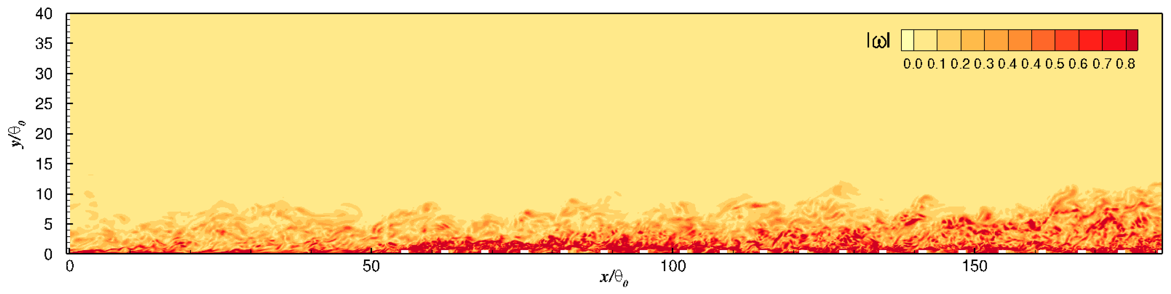
Figure 2.
Inner-scaled (a) mean velocity and (b) RMS velocity fluctuations for the reference case at = 1410. Lines: present results; symbols: data by Schlatter and Örlü (2010) [20].
Figure 2.
Inner-scaled (a) mean velocity and (b) RMS velocity fluctuations for the reference case at = 1410. Lines: present results; symbols: data by Schlatter and Örlü (2010) [20].

Figure 3.
(a) Schematic (side view) of flow setup for the STR DNS (not to scale). (b) A section of the computational domain that represents the staggered distribution of the roughness elements on the bottom wall.
Figure 3.
(a) Schematic (side view) of flow setup for the STR DNS (not to scale). (b) A section of the computational domain that represents the staggered distribution of the roughness elements on the bottom wall.

Figure 4.
Streamwise variation of the normalized pressure gradient in the free stream: (a) normalization by and (b) .
Figure 4.
Streamwise variation of the normalized pressure gradient in the free stream: (a) normalization by and (b) .

Figure 5.
Streamwise variation of frictional velocity (a) and (b) Dashed lines in (b) represent correlation curves of the form , with (case ) and (case ). Filled symbols in (b): experiment by [31]; open symbol in (b): experiment by [32]. (c) Percentage contribution to skin friction . In (c), : viscous drag due to horizontal no-slip surfaces and : viscous drag due to side walls of the roughness elements. (blue line) in (c) indicates the fractional contribution to by horizontal no-slip surfaces at the top of the roughness elements (). The vertical arrows on the –axes indicate the location of the STR step change (SC).
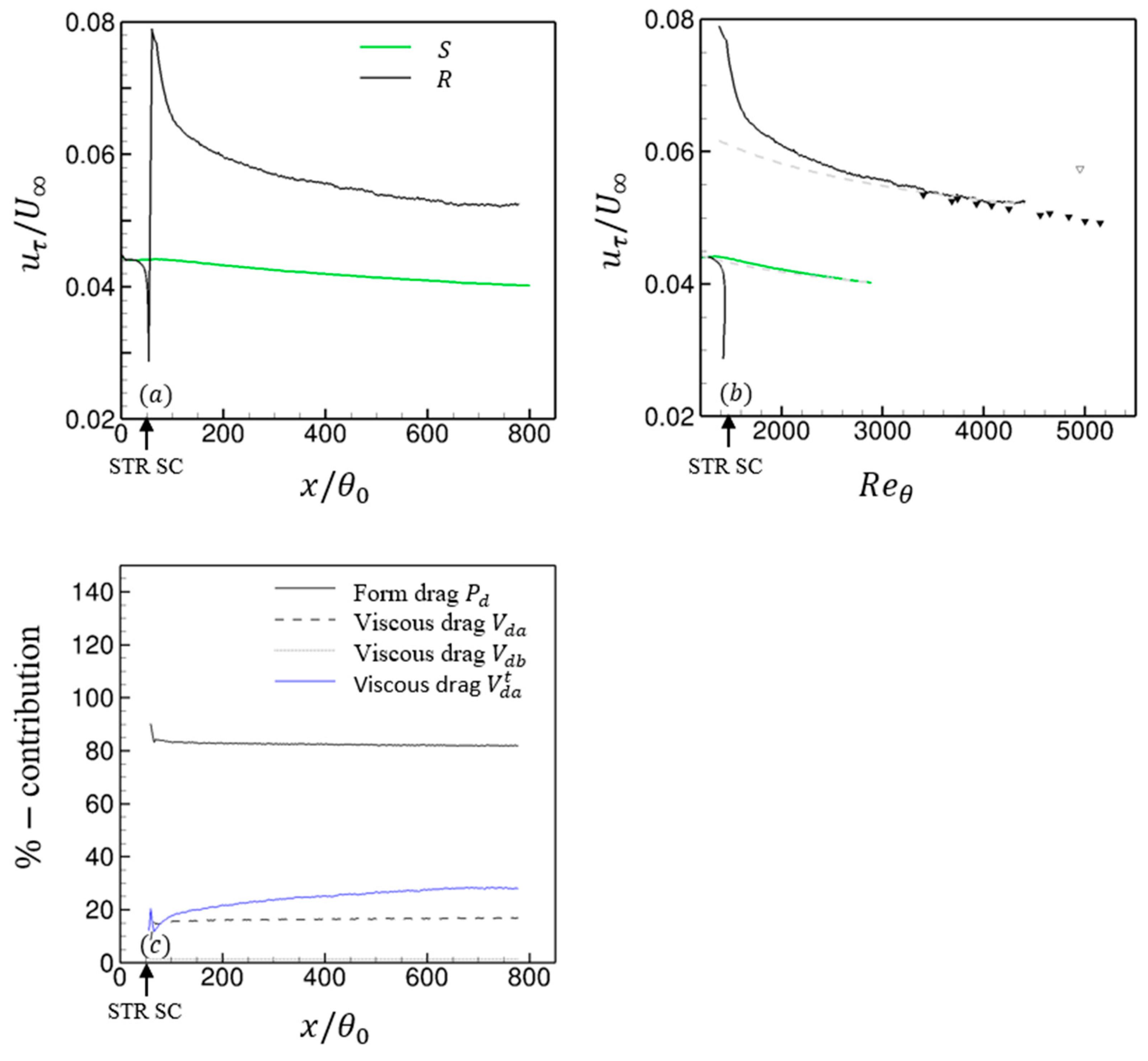
Figure 6.
Mean velocity profiles at select streamwise fetch locations using (a) outer scaling and (b) defect-law scaling for the rough-wall case. The logarithmic equations in (b) correspond to the dashed gray lines. Upstream of the STR step change (green), downstream of the step change (black). Note that the results for reference and the rough-wall cases are identical upstream of the step change at .

Figure 7.
Distribution of on the (a) windward and (b) leeward face of a roughness element. Color contour and solid lines: at ; dashed lines: at . Here, is the reference pressure.
Figure 7.
Distribution of on the (a) windward and (b) leeward face of a roughness element. Color contour and solid lines: at ; dashed lines: at . Here, is the reference pressure.

Figure 8.
(a) Mean velocity profiles at select streamwise fetch locations using inner scaling for the rough-wall case. The logarithmic equations in (a) correspond to the dashed gray lines. Upstream of the STR step change (green), downstream of the step change (black). The location of the profiles follow the legend from Figure 6. Note that the results for reference and the rough-wall cases are identical upstream of the step change at . (b) Streamwise variation of the wake strength parameter .

Figure 9.
Wall normal variation of inner-scaled mean velocity profiles at discrete stations for case . The red solid lines represent the estimated profiles for Coles’ law of the wake: Each profile in red corresponds to a different wake strength parameter , which is extracted from Figure 8.
Figure 9.
Wall normal variation of inner-scaled mean velocity profiles at discrete stations for case . The red solid lines represent the estimated profiles for Coles’ law of the wake: Each profile in red corresponds to a different wake strength parameter , which is extracted from Figure 8.

Figure 10.
Streamwise evolution of momentum thickness (a), displacement thickness (left axis of (b)), and shape factor (right axis of (b)) for the two cases: (green) and (black). In addition, included in (a) is the variation of ratio for the rough-wall case (dashed line). The horizontal arrows indicate the -axis to which each line points to. The vertical arrows on the –axes indicate the location of the STR step change.

Figure 11.
(a) Streamwise variation of as a function of the shape factor for case R. Solid black lines in (a) represent with listed values of . The profile of included in the inset of (a) is calculated using the DNS predictions of and for case R. (b) Evolution of along for case R. Solid black line in (b) presents the relation with . In both (a,b), black squares: (section ; red triangles: (section (ii)); blue circles: (section (iii)).

Figure 12.
Growth of the internal layer along the fetch length . Open circles: estimate of using ; filled squares: estimate of using . Solid line: ; dashed line: power law fit by with exponent being (Rouhi, Chung, and Hutchins [9]); dotted lines: power law fit with exponent and 0.79 (Antonia and Luxton [4]). Inset: normalization is by the local boundary layer thickness The straight line in the inset corresponds to .

Figure 13.
Wall-normal variation of inner-scaled turbulence stresses at different streamwise stations. The wall-normal distance is normalized using the local TBL thickness . (a) Streamwise and wall-normal Reynolds stresses; (b) spanwise Reynolds stress and Reynolds shear stress.
Figure 13.
Wall-normal variation of inner-scaled turbulence stresses at different streamwise stations. The wall-normal distance is normalized using the local TBL thickness . (a) Streamwise and wall-normal Reynolds stresses; (b) spanwise Reynolds stress and Reynolds shear stress.

Figure 14.
Streamwise distribution of (a) (b) , and (c) inside and above a roughness canopy at . The coordinate for the x-axis is defined as where (lines) and (color).
Figure 14.
Streamwise distribution of (a) (b) , and (c) inside and above a roughness canopy at . The coordinate for the x-axis is defined as where (lines) and (color).

Figure 15.
(a) Wall-normal variation of inner-scaled (normalization by TKE budget terms inside and immediately above the canopy at (solid lines) and (dashed lines) for case . (b) Wall-normal variation of outer-scaled (normalization by TKE production and TKE dissipation in the outer layer at (dotted lines), (solid lines), and (dashed lines) for case and at (solid lines with filled symbols) for case . Only data from above the canopy are presented for case in (b). Profiles in (a,b) are extracted from the spanwise center of a repeating unit.

Figure 16.
(a) Ratio of contribution to the turbulence shear stress by to . (b) Percentage of total time spent as bursts (inset: percentage of total time spent as sweeps). The lines in (b) follow the labels from (a). Profiles for case are only presented for the wall-normal extent above the canopy.
Figure 16.
(a) Ratio of contribution to the turbulence shear stress by to . (b) Percentage of total time spent as bursts (inset: percentage of total time spent as sweeps). The lines in (b) follow the labels from (a). Profiles for case are only presented for the wall-normal extent above the canopy.

Figure 17.
Instantaneous streamwise fluctuations in an plane at . Top panel ; bottom panel: . Solid lines on top of the color contours indicate = 0.1.
Figure 17.
Instantaneous streamwise fluctuations in an plane at . Top panel ; bottom panel: . Solid lines on top of the color contours indicate = 0.1.

Figure 18.
Visualization of iso-surfaces of the –criterion at (top panel) and (bottom panel). The iso-surfaces are colored by the wall normal distance: (yellow); (red). (Top panel): ; (bottom panel): . Only about 1/3rd of the entire spanwise domain is presented.
Figure 18.
Visualization of iso-surfaces of the –criterion at (top panel) and (bottom panel). The iso-surfaces are colored by the wall normal distance: (yellow); (red). (Top panel): ; (bottom panel): . Only about 1/3rd of the entire spanwise domain is presented.

Figure 19.
Wall-normal variation of the (a) integral length scale and (b) inner-scaled integral timescale at different streamwise stations above the rough and smooth walls. The profiles for and in (a) are shifted vertically while those for in (b) are multiplied by to provide clarity. Open symbols in (b): data by Quadrio and Luchini (2003) [56] at .

Figure 20.
Wall-normal variation of the integral timescale ratio at discrete streamwise stations for cases and .
Figure 20.
Wall-normal variation of the integral timescale ratio at discrete streamwise stations for cases and .


Table 1.
Details on the construction of the domain and grid resolution. The subscripts and with imply the grid spacing at the wall and at local TBL height, respectively.
Table 1.
Details on the construction of the domain and grid resolution. The subscripts and with imply the grid spacing at the wall and at local TBL height, respectively.
| Case | |||||
|---|---|---|---|---|---|
| |11.7 | |||||
| |10.5 | 13.1 |
Disclaimer/Publisher’s Note: The statements, opinions and data contained in all publications are solely those of the individual author(s) and contributor(s) and not of MDPI and/or the editor(s). MDPI and/or the editor(s) disclaim responsibility for any injury to people or property resulting from any ideas, methods, instructions or products referred to in the content. |
© 2023 by the author. Licensee MDPI, Basel, Switzerland. This article is an open access article distributed under the terms and conditions of the Creative Commons Attribution (CC BY) license (https://creativecommons.org/licenses/by/4.0/).
Share and Cite
MDPI and ACS Style
Ismail, U. Direct Numerical Simulation of a Turbulent Boundary Layer Encountering a Smooth-to-Rough Step Change. Energies 2023, 16, 1709. https://doi.org/10.3390/en16041709
AMA Style
Ismail U. Direct Numerical Simulation of a Turbulent Boundary Layer Encountering a Smooth-to-Rough Step Change. Energies. 2023; 16(4):1709. https://doi.org/10.3390/en16041709
Chicago/Turabian StyleIsmail, Umair. 2023. "Direct Numerical Simulation of a Turbulent Boundary Layer Encountering a Smooth-to-Rough Step Change" Energies 16, no. 4: 1709. https://doi.org/10.3390/en16041709
Note that from the first issue of 2016, this journal uses article numbers instead of page numbers. See further details here.